Reliability Test Plan for an Extended Birnbaum-Saunders Distribution

Jiju Gillariose^1,* and Lishamol Tomy²

¹Department of Statistics, St.Thomas College, Pala, Kerala-686574, India

²Department of Statistics, Deva Matha College, Kuravilangad, Kerala-686633, India

E-mail: jijugillariose@yahoo.com; lishatomy@gmail.com

*Corresponding Author

Received 20 November 2020; Accepted 17 March 2021; Publication 22 June 2021

Abstract

Birnbaum-Saunders distribution has been widely studied in statistical literature because this distribution accommodates several interesting properties. The purpose of this paper is to introduce a new parametric distribution based on the Birnbaum-Saunders model and develop a new acceptance sampling plans for derived extended Birnbaum-Saunders distribution when the mean lifetime test is truncated at a predetermined time. For various acceptance numbers, confidence levels and values of the ratio of the fixed experimental time to the specified mean life, the minimum sample size necessary to assure a specified mean lifetime worked out. The results are illustrated by a numerical example. The operating characteristic functions of the sampling plans and producer’s risk and the ratio of true mean life to a specified mean life that ensures acceptance with a pre-assigned probability are tabulated. This paper presents relevant characteristics of the new distribution and a new acceptance sampling plans when the lifetime of a product adopts an extended Birnbaum-Saunders distribution. Based on this study, the optimal number of testers demanded is decreases as test termination time increases. Moreover, the operating characteristic values increases as the mean life ratio increases, which indicate that items with increased mean life will be accepted with higher probability compared with items with lower mean life ratio.

Keywords: Birnbaum-Saunders distribution, maximum likelihood estimation, operating characteristics function, reliability test plan, truncated negative binomial distribution.

1 Introduction

Birnbaum and Saunders (1969a,1969b) invented the Birnbaum-Saunders (BS) distribution for the purpose of modeling fatigue failures caused by periodic stresses. The BS distribution is derived by making a monotone transformation on the standard normal random variable and it is also called fatigue-life distribution. The random variable $X$ is said to have the BS distribution with parameters $\alpha$ and $\beta$, the shape and scale parameters respectively, if its cumulative distribution function (CDF) is given by

$$F(x)=\mathrm{\Phi }(\mu ),x,\alpha ,\beta >0$$

(1)

where $\mathrm{\Phi }(\cdot )$ is the standard normal CDF and $\mu ={\alpha }^{-1}\{{[\frac{x}{\beta }]}^{1/2}-{[\frac{x}{\beta }]}^{-1/2}\}$. If the random variable $X$ has the BS distribution function in (1), then the associated probability density function (PDF) and hazard rate function (HRF) are given by

$$f(x,\alpha ,\beta )=\frac{1}{2\sqrt{2\pi }\alpha \beta }\left\{{\left[\frac{\beta }{x}\right]}^{1/2}+{\left[\frac{\beta }{x}\right]}^{3/2}\right\}{e}^{-\frac{1}{2{\alpha }^2}\left\{\frac{x}{\beta }+\frac{\beta }{x}-2\right\}},$$
$$x,\alpha ,\beta >0$$	(2)

and

$$h(x,\alpha ,\beta )=\frac{\left\{{\left[\frac{\beta }{x}\right]}^{1/2}+{\left[\frac{\beta }{x}\right]}^{3/2}\right\}{e}^{-\frac{1}{2{\alpha }^2}\left\{\frac{x}{\beta }+\frac{\beta }{x}-2\right\}}}{2\sqrt{2\pi }\alpha \beta \mathrm{\Phi }(-\mu )},x,\alpha ,\beta >0$$

(3)

The PDF and HRF of the BS distribution is unimodal for all values of $\alpha$ and $\beta$. The maximum likelihood estimators (mle) of the shape and scale parameters based on a complete sample were discussed originally by Birnbaum and Saunders (1969b). Various statistical experts have mentioned results associated with BS distribution. Desmond (2012) observed a relationship between BS and Inverse Gaussian distribution. Ng et al. (2003) performed extensive Monte Carlo simulations to compare the performances of the mles and method of moments estimators. Balakrishnan et al. (2010) studied the properties of a mixture of two BS distributions. For more details of the BS distribution, interested reader can refer the recent book by Leiva (2016).

In the last few years, new classes of distributions have been found by extending BS distribution. Because of its increasing popularity, the main objective of this paper is to propose and derive a generalization of BS distribution. Nadarajah et al. (2012) introduced a new family of distributions, by adding two parameters to baseline distribution. Let $X_1,X_2,\mathrm{\dots }$ be a sequence of independent and identically distributed random variables with survival function $\overline{F}(x)$ and $N$ be a truncated negative binomial random variable, independent of $X_i$’s, with parameters $0<\theta <1$ and $\lambda >0$ (Nadarajah et al. 2012), then

$$P(N=n)=\frac{{\theta }^{\lambda }}{1-{\theta }^{\lambda }}\left(\begin{array}{c}\lambda +n-1\hfill \\ \lambda -1\hfill \end{array}\right){(1-\theta )}^n;n=1,2,\mathrm{\dots }$$

(4)

If $U_N=min(X_1,X_2,\mathrm{\dots }{X}_N$), then the survival function of $U_N$ is

$$\overline{G}(x,\theta ,\lambda )=\frac{{\theta }^{\lambda }}{1-{\theta }^{\lambda }}\{{[F(x)+\theta \overline{F}(x)]}^{-\lambda }-1\}x\in R,\theta ,\lambda >0$$

(5)

Similarly, if $\theta >1$ and $N$ is a truncated negative binomial random variable with parameters $\frac{1}{\theta }$ and $\lambda >0$, then $W_N=max(X_1,X_2,\mathrm{\dots }{X}_N$) also has the same survival function given in (4). If $\theta \to 1$ in (4), then $\overline{G}(x,\theta ,\lambda )\to \overline{F}(x)$. If $\lambda =1$, then this family reduces to the Marshall-Olkin family of distributions proposed by Marshall-Olkin (1997). Clearly the PDF corresponding to the survival function in Equation (4) is given by

$$g(x,\theta ,\lambda )=\frac{(1-\theta )\lambda {\theta }^{\lambda }f(x)}{(1-{\theta }^{\lambda }){\{F(x)+\theta \overline{F}(x)\}}^{\lambda +1}}$$

(6)

A number of statistical researchers have been proposed new distributions using this family. Jose and Sivadas (2015) constructed the negative binomial Marshall-Olkin Rayleigh distribution. Jayakumar and Sankaran (2016) defined a generalized uniform distribution using the approach of Nadarajah et al. (2012). Babu (2016) introduced Weibull truncated negative binomial distribution. Further, Jayakumar and Sankaran (2017) developed generalized exponential truncated negative binomial distribution and studied its properties. Moreover, Jiju and Lishamol (2018) introduced generalized Rayleigh truncated negative binomial distribution. Furthermore, Al-Omari et al. presented acceptance sampling plans based on truncated life tests for Rama distribution.

The outline of the paper is as follows. Section 2 deals with the new distribution and its statistical properties. Section 3 provides estimation of parameters using mle method and real data application illustrate the performance of the distribution. Section 4 gives sampling plan for accepting or rejecting a lot and minimum samples sizes and operating characteristic values are calculated and a numerical example is provided. The concluding remarks are made in Section 5.

2 Birnbaum-Saunders Truncated Negative Binomial Distribution

In this section, we develop a new distribution namely Birnbaum-Saunders Truncated Negative Binomial (BS-TNB) distribution, by inserting (1) in (4), the survival function of BS-TNB distribution is given by

$\overline{G}(x,\alpha ,\beta ,\lambda ,\theta )={\displaystyle \frac{{\theta }^{\lambda }}{1-{\theta }^{\lambda }}}\{{[\mathrm{\Phi }(\mu )+\theta \mathrm{\Phi }(-\mu )]}^{-\lambda }-1\}x,\alpha ,\beta ,\theta ,\lambda >0$ (7)

The corresponding PDF is given by

$$g(x,\alpha ,\beta ,\lambda ,\theta )=\frac{(1-\theta )\lambda {\theta }^{\lambda }}{2\sqrt{2\pi }\alpha \beta }\frac{\left\{{\left[\frac{\beta }{x}\right]}^{1/2}+{\left[\frac{\beta }{x}\right]}^{3/2}\right\}{e}^{-\frac{1}{2{\alpha }^2}\left\{\frac{x}{\beta }+\frac{\beta }{x}-2\right\}}}{(1-{\theta }^{\lambda }){\left\{\mathrm{\Phi }(\mu )+\theta \mathrm{\Phi }(-\mu )\right\}}^{\lambda +1}}$$
$$x,\alpha ,\beta ,\theta ,\lambda >0$$	(8)

In addition, the HRF of the BS-TNB distribution becomes

$h(x,\alpha ,\beta ,\lambda ,\theta )$
$\mathrm{\hspace{1em}\hspace{1em}}={\displaystyle \frac{(1-\theta )\lambda }{2\sqrt{2\mathrm{\Pi }}\alpha \beta }}{\displaystyle \frac{\left\{{\left[\frac{\beta }{x}\right]}^{1/2}+{\left[\frac{\beta }{x}\right]}^{3/2}\right\}{e}^{-\frac{1}{2{\alpha }^2}\left\{\frac{x}{\beta }+\frac{\beta }{x}-2\right\}}}{{\left\{\mathrm{\Phi }(\mu )+\theta \mathrm{\Phi }(-\mu )\right\}}^{\lambda +1}\left\{{[\mathrm{\Phi }(\mu )+\theta \mathrm{\Phi }(-\mu )]}^{-\lambda }-1\right\}}}$
$\mathrm{\hspace{1em}\hspace{1em}}x,\alpha ,\beta ,\theta ,\lambda >0$	(9)

Figures 1 displays some shapes of PDF of the BS-TNB model for selected parameter values. It is clear that the BS-TNB distribution is much more flexible than the BS distribution. Plots of the HRF for different parameter values are displayed in Figure 2. We note that these plots illustrate the classic types of hazard shapes, which is relevant because there are fewer lifetime distributions that shows shapes similar to this.

Figure 1 Graphs of PDF of the BS-TNB distribution for different values of $\alpha$,$\beta$,$\lambda$ and $\theta$.

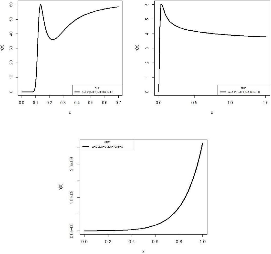
Figure 2 Graphs of HRF of the BS-TNB distribution for different values of $\alpha$,$\beta$,$\lambda$ and $\theta$.

The quantile function of $X$ follows BS-TNB distribution, it can be expressed as

$Q(u)$	$={\displaystyle \frac{\beta }{4}}[\alpha {\mathrm{\Phi }}^{-1}\left[{\displaystyle \frac{\theta }{1-\theta }}\{{(1+p({\theta }^{\lambda }-1))}^{-\frac{1}{\lambda }}-1\}\right]$
	$+\sqrt{{\left(\alpha {\mathrm{\Phi }}^{-1}\left[{\displaystyle \frac{\theta }{1-\theta }}\left\{{\left(1+p({\theta }^{\lambda }-1)\right)}^{-\frac{1}{\lambda }}-1\right\}\right]\right)}^2+4}]{}^2$

where $u$ is generated from the Uniform(0,1) distribution and ${\mathrm{\Phi }}^{-1}(\cdot )$ is the quantile function of the standard normal with CDF $\mathrm{\Phi }(\cdot )$.

3 Estimation and Application

3.1 Maximum Likelihood Estimation

Let $X_1,X_2,\mathrm{\dots },X_n$ is a random sample of size n from the BS-TNB distribution with parameters $\alpha ,\beta ,\lambda$ and $\theta$. Let $\mathrm{\Phi }={(\alpha ,\beta ,\lambda ,\theta )}^T$ be the $p\times 1$ parameter vector. For determining the MLEs of $\alpha ,\beta ,\lambda$ and $\theta$, we have the log-likelihood function

$logl(\mathrm{\Phi })$	$=nlog(1-\theta )+nlog\lambda +n\lambda log\theta -nlog(2\sqrt{2\mathrm{\Pi }})$
	$\mathrm{\hspace{1em}}-nlog\alpha -nlog\beta -nlog(1-{\theta }^{\lambda })$
	$\mathrm{\hspace{1em}}+{\displaystyle \sum _i^n}\left(log\left\{{\left[{\displaystyle \frac{\beta }{x_i}}\right]}^{1/2}+{\left[{\displaystyle \frac{\beta }{x_i}}\right]}^{3/2}\right\}\right)$
	$\mathrm{\hspace{1em}}-{\displaystyle \frac{1}{2{\alpha }^2}}{\displaystyle \sum _i^n}\left\{{\displaystyle \frac{x_i}{\beta }}+{\displaystyle \frac{\beta }{x_i}}-2\right\}-(\lambda +1){\displaystyle \sum _i^n}log\left\{1-\overline{\theta }\mathrm{\Phi }(-{\mu }_i)\right\}$

The components of the score vector, $U(\mathrm{\Phi })=\frac{\partial \log l}{\partial \mathrm{\Phi }}=(U_{\alpha }=\frac{\partial \log l}{\partial \alpha },U_{\beta }=\frac{\partial \log l}{\partial \beta }$, $U_{\lambda }=\frac{\partial \log l}{\partial \lambda }$, $U_{\theta }=\frac{\partial \log l}{\partial \theta }){}^T$ are given by

$U_{\alpha }$	$=-{\displaystyle \frac{n}{\alpha }}-{\displaystyle \frac{1}{{\alpha }^3}}{\displaystyle \sum _{i=1}^n}\left\{{\displaystyle \frac{x_i}{\beta }}+{\displaystyle \frac{\beta }{x_i}}-2\right\}$
	$\mathrm{\hspace{1em}}+{\displaystyle \frac{(\lambda +1)\overline{\theta }}{{\alpha }^2}}{\displaystyle \sum _i^n}{\displaystyle \frac{\varphi (-{\mu }_i)\{{[\frac{x_i}{\beta }]}^{1/2}-{[\frac{\beta }{x_i}]}^{1/2}\}}{\left\{1-\overline{\theta }\mathrm{\Phi }(-{\mu }_i)\right\}}}$
$U_{\beta }$	$=-{\displaystyle \frac{n}{2\beta }}+{\displaystyle \sum _{i=1}^n}{\displaystyle \frac{1}{x_i+\beta }}+{\displaystyle \frac{1}{2{\alpha }^2\beta }}{\displaystyle \sum _{i=1}^n}\left[{\displaystyle \frac{x_i}{\beta }}-{\displaystyle \frac{\beta }{x_i}}\right]$
	$\mathrm{\hspace{1em}}+{\displaystyle \frac{(\lambda +1)\overline{\theta }}{2\alpha \beta }}{\displaystyle \sum _i^n}{\displaystyle \frac{\varphi (-{\mu }_i)\{{[\frac{x_i}{\beta }]}^{1/2}+{[\frac{\beta }{x_i}]}^{1/2}\}}{\left\{1-\overline{\theta }\mathrm{\Phi }(-{\mu }_i)\right\}}}$
$U_{\lambda }$	$={\displaystyle \frac{n}{\lambda }}+{\displaystyle \frac{n\lambda }{\theta }}+{\displaystyle \frac{n{\theta }^{\lambda }log\theta }{1-{\theta }^{\lambda }}}-{\displaystyle \sum _{i=1}^n}log\left\{1-\overline{\theta }\mathrm{\Phi }(-{\mu }_i)\right\}$
$U_{\theta }$	$={\displaystyle \frac{n}{1-\theta }}+{\displaystyle \frac{n\lambda }{\theta }}-{\displaystyle \frac{n\lambda {\theta }^{\lambda -1}}{1-{\theta }^{\lambda }}}$
	$\mathrm{\hspace{1em}}-(\lambda +1){\displaystyle \sum _{i=1}^n}{\displaystyle \frac{\mathrm{\Phi }({\mu }_i)}{\left\{1-\overline{\theta }\mathrm{\Phi }(-{\mu }_i)\right\}}}$

where $\varphi (\cdot )$ is the standard normal density function and $\mathrm{\Phi }(-\mu )$ is the survival function of BS distribution. Solving simultaneously $U_{\alpha }=0$, $U_{\beta }=0$, $U_{\theta }=0$ and $U_{\lambda }=0$ gives the MLEs of $\widehat{\mathrm{\Phi }}$. These equations can be solved using any statistical softwares.

3.2 Real Data Application

In this section, we present an application of the BS-TNB distribution to illustrate its usefulness. The real data set corresponds to the daily ozone measurements in New York, May-September 1973 reported in Nadarajah (2008).

The data are: 41, 36, 12, 18, 28, 23, 19, 8, 7, 16, 11, 14, 18, 14, 34, 6, 30, 11, 1, 11, 4, 32, 23, 45, 115, 37, 29, 71, 39, 23, 21, 37, 20,12, 13, 135, 49, 32, 64, 40, 77, 97, 97, 85, 10, 27, 7, 48, 35, 61, 79, 63, 16, 80, 108, 20,52, 82, 50, 64, 59, 39, 9, 16, 78, 35, 66, 122, 89, 110, 44, 28, 65, 22, 59, 23, 31, 44, 21, 9,45, 168, 73, 76, 118, 84, 85, 96, 78, 73, 91, 47, 32, 20, 23, 21, 24, 44, 21, 28, 9, 13, 46,18, 13, 24, 16, 13, 23, 36, 7, 14, 30, 14, 18, 20.

All computations are performed using the R software. We compare BS-TNB distribution with BS distribution so that we estimated the unknown parameters (by the maximum likelihood method), the values of the $-$log-likelihood ($-$logL), AIC (Akaike Information Criterion), BIC (Bayesian Information Criterion), Kolmogrov-Smirnov (K-S) statistic and $p$-value.

The resulted values for the data are given in Table 1. From these results, we can observe that BS-TNB distribution presents the smaller value of $-$logL, AIC BIC, K-S and the largest $p$-value. Therefore, we can conclude that the BS-TNB distribution gives the best fit to the current data.

Table 1 Comparison criterion for the data set

Distribution	Estimates (SE)	$-\log L$	AIC	BIC	K-S	$p$-value
BS-TNB	$\widehat{a}=1.3726$ (0.3284)	541.1454	1091.895	1102.909	0.0730	0.5651
($a,b,\lambda ,\rho$)	$\widehat{b}=8.9100$ (4.6544)
	$\widehat{\rho }=1.0300$ (0.1404)
	$\widehat{\lambda }=137.69$ (579.10)
BS($a,b$)	$\widehat{a}=0.9825$ (0.0645)	549.0972	1102.194	1107.702	0.0829	0.4020
	$\widehat{b}=28.0314$ (2.2658)

4 Acceptance Sampling Plans

Product quality is an essential tool for its acceptability. Products with high quality have higher acceptability compared with products with low quality. Therefore the quality becomes momentous tool between competitive enterprisers in a global market. The quality supervisors had to make sure that the products supplied to the customers are of high quality and also ensure that the market receives shipments that do not contain defective products. Acceptance sampling in quality control is an important techniques for ensuring the quality. It is a specific plan that establishes the minimum sample size to be used and the associated acceptance and non-acceptance criteria for the manufacturing products. The basis for the acceptance sampling plans has been discussed in detail by Epstein (1954), see also Sobel and Tischendrof (1959).

4.1 Reliability Test Plan with BS-TNB Lifetime

In this section, we develop reliability test plan with lifetime follows the BS-TNB distribution with CDF

$G(t,\alpha ,\lambda ,\theta \beta ,)=1-{\displaystyle \frac{{\theta }^{\lambda }}{1-{\theta }^{\lambda }}}\{{[\mathrm{\Phi }(\mu )+\theta \overline{\mathrm{\Phi }}(\mu )]}^{-\lambda }-1\}t,\alpha ,\beta ,\theta ,\lambda >0$

(10)

A common practice in life testing is to terminate the life test by a pre-fixed time t and noted the number of failures. One of the objectives of these experiments is to set a lower confidence limit on the average life. It is then desired to establish a specified average life with a given probability of at least $p^{*}$. The decision to accept the specified average life occurs if and only if the number of observed failures at the end of the fixed time t does not exceed an acceptance number $c$. The test may get terminated before the time t is reached when the number of failures exceeds c in which case the decision is to reject the lot. For such a truncated life test and the associated decision rule, we are interested in obtaining the smallest sample sizes necessary to achieve the objective. Here we assume that $\alpha ,\theta$ and $\lambda$ are known while $\beta$ is unknown. So average lifetime depends only on $\beta$. A sampling plan consists of

• the number of units $n$ on test,

• the acceptance number $c$,

• the maximum test duration $t$, and

• the ratio $\frac{t}{{\beta }_0}$ where ${\beta }_0$ is the specified average life.

The consumer’s risk not to exceed $1-p^{*}$, so that $p^{*}$ is a minimum confidence level with which a lot of true average life below ${\beta }_0$ is rejected, by the sampling plan. For a fixed $p^{*}$ our sampling plan is characterized by ($n$, $c$, $\frac{t}{{\beta }_0}$). Here we consider sufficiently large lots so that the binomial distribution can be applied. The problem is to determine for given values of $p^{*}$, $(0<p^{*}<1)$, ${\beta }_0$ and $c$ the smallest positive integer $n$ such that

$$\sum _{i=0}^c\left(\begin{array}{c}n\hfill \\ i\hfill \end{array}\right)p^i{(1-p)}^{n-i}\le 1-p^{*}$$

(11)

holds where $p=G(t,\alpha ,\theta ,\lambda ,{\beta }_0)$ is given by (9) indicates the failure probabilities before time t which depends only on the ratio $t/{\beta }_0$ it is sufficient to specify this ratio for designing the experiment. If the number of observed failures before $t$ is less than or equal to $c$, from (10) we obtain:

$$G(t,\beta )\le G(t,{\beta }_0)⟺\beta \ge {\beta }_0$$

(12)

The minimum values of n which satisfies the inequality (11) are for $p^{*}=0.75$, 0.90, 0.95, .99 and $t=0.628$, 0.942, 1.257, 1.571, 2.356, 3.141, 3.927, 4.712 and $\alpha =\lambda =1,\theta =2$ obtained and presented in Table 2. If $p=G(t,\alpha ,\theta ,\lambda ,{\beta }_0)$ is small and $n$ is large (as is true in some cases of our present work), the binomial probability may be approximated by Poisson probability with parameter $\eta =np$ so that the left side of (11) can be written as

$$\sum _{i=0}^c\frac{e^{-\mu }{\mu }^x}{x}\le 1-p^{*}$$

(13)

where $p=G(t,\alpha ,\theta ,\lambda ,{\beta }_0)$. The minimum values of $n$ satisfying (12) are obtained for the same combination of $p$ values as those used for (11). The results are given in Table 3.

The operating characteristic (OC) function of the sampling plan $(n,c,t/{\beta }_0)$ provides the probability $L(p)$ of accepting the lot with:

$$L(p)=P(\mathrm{Accepting}\mathrm{a}\mathrm{lot})=\sum _{i=0}^c\left(\begin{array}{c}n\hfill \\ i\hfill \end{array}\right)p^i{(1-p)}^{n-i}$$

(14)

where $p=G(t,\alpha ,\beta ,\lambda ,\theta )$ is considered as a function of the lot quality parameter $\beta$. For given $p^{*}$, $t/{\beta }_0$ the choice of c and n is made on the basis of OC. Values of the OC as a function of $W=\beta /{\beta }_0$ for a few sampling plans are given in Table 4.

The producers risk is the probability of rejecting lot when $\beta >{\beta }_0$. We can compute the producers risk by first finding $p=F(t,\beta )$ and then using the binomial distribution function. For a given value of the producers risk say 0.05, one may be interested in knowing what value of $\beta /{\beta }_0$ will ensure a producers risk less than or equal to 0.05 if a sampling plan under discussion is adopted. It should be noted that the probability p may be obtained as function of $\beta /{\beta }_0$, as

$$p=G(\frac{t}{{\beta }_0}\frac{{\beta }_0}{\beta })$$

(15)

The value $\theta /{\theta }_0$ is the smallest positive number for which the following inequality hold:

$$\sum _{i=0}^c\left(\begin{array}{c}n\hfill \\ i\hfill \end{array}\right)p^i{(1-p)}^{n-i}\ge .95$$

(16)

For a given sampling plan (n, c, $t/{\beta }_0$) and specified confidence level $p^{*}$. the minimum values of $\beta /{\beta }_0$ satisfying the inequality (15) are given in Table 5.

Table 2 Minimum sample sizes necessary to assert the average life to exceed a given value $t/{\beta }_0$ with probability $p^{*}$ and the corresponding acceptance number $c$, $\alpha =\lambda =1,\theta =2$ using Binomial probabilities

	$t/{\beta }_0$
$p^{*}$	$c$	0.628	0.942	1.257	1.571	2.356	3.141	3.972	4.712
0.75	0	7	4	3	2	2	1	1	1
	1	14	8	6	5	3	3	2	2
	2	20	12	9	7	5	4	4	3
	3	26	16	12	9	7	6	5	5
	4	32	19	14	11	8	7	6	6
	5	38	23	17	13	10	8	7	7
	6	45	27	20	15	11	10	9	8
	7	51	30	22	17	13	11	10	9
	8	60	34	25	19	15	12	11	10
	9	63	37	27	22	16	14	12	11
	10	67	41	30	24	18	15	13	12
0.90	0	11	7	5	4	3	2	2	1
	1	20	11	8	7	5	4	3	3
	2	27	16	11	9	6	5	4	4
	3	34	20	14	12	8	7	6	5
	4	40	24	17	15	10	8	7	6
	5	47	28	20	18	11	9	8	8
	6	54	32	23	20	13	11	9	9
	7	60	36	26	22	15	12	11	10
	8	66	39	29	23	16	14	12	11
	9	73	43	32	25	18	15	13	12
	10	79	47	34	28	20	16	14	13
0.95	0	15	8	6	5	3	2	2	2
	1	24	14	10	8	5	4	3	3
	2	31	18	13	10	7	6	5	4
	3	39	23	16	13	9	7	6	6
	4	46	27	20	16	11	9	7	7
	5	53	31	23	18	13	10	9	8
	6	60	35	26	20	14	12	10	9
	7	66	39	28	23	16	13	11	10
	8	73	43	31	25	18	14	13	12
	9	80	47	34	27	19	16	14	13
	10	86	51	37	30	20	17	15	14
0.99	0	22	13	9	7	5	4	3	2
	1	33	19	13	10	7	5	4	4
	2	41	24	17	13	9	7	6	5
	3	50	29	21	16	11	9	7	6
	4	58	34	24	19	13	10	9	8
	5	66	39	27	22	15	12	10	9
	6	73	43	31	24	17	13	11	10
	7	80	47	34	27	18	15	13	11
	8	87	51	37	30	20	16	14	13
	9	94	55	40	32	22	18	15	14
	10	101	60	43	34	24	19	17	15

Table 3 Minimum sample sizes necessary to assert the average life to exceed a given value $t/{\beta }_0$ with probability $p^{*}$ and the corresponding acceptance number $c$, $\alpha =\lambda =1,\theta =2$ using Poisson probabilities

	$t/{\beta }_0$
$p^{*}$	$c$	0.628	0.942	1.257	1.571	2.356	3.141	3.972	4.712
0.75	0	8	5	4	3	3	2	2	2
	1	15	9	7	6	4	4	4	3
	2	21	13	10	8	6	5	5	4
	3	27	17	13	11	8	7	6	6
	4	34	21	15	13	10	8	8	7
	5	40	24	18	15	12	10	9	8
	6	46	28	21	17	13	11	10	9
	7	51	31	24	19	15	13	12	10
	8	57	35	26	22	16	14	13	11
	9	63	39	29	24	18	15	14	12
	10	69	42	32	26	20	17	15	14
0.95	0	13	8	6	5	4	3	3	3
	1	21	13	10	8	6	5	5	5
	2	30	18	13	11	8	7	7	6
	3	36	22	16	14	10	9	8	8
	4	43	26	20	16	12	11	10	9
	5	49	30	23	19	14	12	11	11
	6	56	34	26	21	16	14	13	12
	7	62	38	29	24	18	15	14	13
	8	69	42	32	26	20	17	15	15
	9	75	46	35	28	21	18	17	16
	10	82	50	37	31	23	20	18	17
0.95	0	16	10	8	6	5	4	4	4
	1	25	16	12	10	7	6	6	6
	2	34	21	16	13	10	8	8	7
	3	41	25	19	16	12	10	9	9
	4	49	30	22	18	14	12	11	10
	5	56	34	26	21	16	14	13	12
	6	63	38	29	24	18	15	14	13
	7	70	43	32	26	20	17	16	15
	8	76	47	35	29	22	19	17	16
	9	83	51	38	31	24	20	18	18
	10	90	55	41	34	25	22	20	19
0.99	0	25	15	11	10	7	6	6	5
	1	35	22	16	14	10	9	8	7
	2	45	27	21	17	13	11	10	9
	3	53	33	24	20	15	13	12	11
	4	62	38	28	23	17	15	14	12
	5	70	43	32	26	20	17	16	14
	6	77	47	35	29	22	19	17	15
	7	85	52	39	32	24	21	19	17
	8	92	56	42	35	26	22	20	18
	9	99	61	45	37	28	24	22	19
	10	107	65	49	40	30	26	24	21

Table 4 Operating characteristic values of the sampling plan ($n,c,t/{\beta }_0$) for given $p^{*}$ and $\alpha =\lambda =1,\theta =2$ under BS-TNB probabilities

	$\beta /{\beta }_0$
$p^{*}$	$n$	$c$	$t/{\beta }_0$	2	4	6	8	10	12
0.75	20	2	0.628	0.8916	0.9994	1	1	1	1
	12	2	0.942	0.8215	0.9953	0.9999	1	1	1
	9	2	1.257	0.7636	0.9871	0.9992	1	1	1
	7	2	1.571	0.7492	0.9803	0.9982	0.9998	1	1
	5	2	2.356	0.6931	0.9602	0.9935	0.9988	0.9998	0.9999
	4	2	3.141	0.6723	0.9473	0.9889	0.9972	0.9992	0.9998
	4	2	3.972	0.5071	0.8911	0.9712	0.9912	0.997	0.9989
	3	2	4.712	0.6817	0.9389	0.9837	0.9947	0.9981	0.9993
0.90	27	2	0.628	0.7924	0.9985	1	1	1	1
	16	2	0.942	0.6824	0.9891	0.9997	1	1	1
	11	2	1.257	0.6374	0.9749	0.9984	0.9999	1	1
	9	2	1.571	0.5911	0.9587	0.9959	0.9996	1	1
	6	2	2.356	0.5571	0.9306	0.9879	0.9977	0.9995	0.9999
	5	2	3.141	0.4812	0.8929	0.9752	0.9935	0.9982	0.9995
	4	2	3.972	0.5071	0.8911	0.9712	0.9912	0.997	0.9989
	4	2	4.712	0.3788	0.8278	0.9473	0.9817	0.9931	0.9972
0.95	31	2	0.628	0.7291	0.9978	1	1	1	1
	18	2	0.942	0.611	0.9848	0.9996	1	1	1
	13	2	1.257	0.538	0.9631	0.9976	0.9998	1	1
	10	2	1.571	0.5153	0.9449	0.9943	0.9994	0.9999	1
	7	2	2.356	0.4333	0.8939	0.9803	0.9961	0.9992	0.9998
	6	2	3.141	0.3251	0.8253	0.9558	0.9879	0.9965	0.9989
	5	2	3.972	0.2999	0.7938	0.9389	0.9802	0.9931	0.9975
	4	2	4.712	0.3788	0.8278	0.9473	0.9817	0.9931	0.9972
0.99	41	2	0.628	0.5676	0.995	1	1	1	1
	24	2	0.942	0.4148	0.9669	0.9989	1	1	1
	17	2	1.257	0.3459	0.9263	0.9946	0.9996	1	1
	13	2	1.571	0.3223	0.8928	0.9876	0.9986	0.9998	1
	9	2	2.356	0.2435	0.8047	0.9588	0.9912	0.9981	0.9996
	7	2	3.141	0.2104	0.7495	0.9309	0.9803	0.9941	0.9982
	6	2	3.972	0.1654	0.6853	0.8961	0.9644	0.9872	0.9952
	5	2	4.712	0.1866	0.6931	0.8929	0.9602	0.9843	0.9935

Table 5 Minimum ratio of true $\beta$ and required ${\beta }_0$ for the acceptability of a lot with producer’s risk of 0.05 for $\alpha =\lambda =1,\theta =2$ under BS-TNB probabilities

	$t/{\beta }_0$
$p^{*}$	$c$	0.628	0.942	1.257	1.571	2.356	3.141	3.972	4.712
0.75	0	4.2	5.42	6.62	7.11	10.66	10.75	13.59	16.12
	1	2.8	3.38	3.95	4.58	4.85	6.47	5.66	6.72
	2	2.37	2.96	3.12	3.32	3.9	4.18	5.29	4.38
	3	2.08	2.41	2.72	2.82	3.36	3.79	3.9	4.62
	4	1.98	2.27	2.36	2.5	2.76	3.08	3.23	3.84
	5	1.83	2.04	2.26	2.24	2.59	2.62	2.78	3.3
	6	1.77	1.97	2.12	2.09	2.31	2.69	2.92	2.93
	7	1.71	1.85	1.96	1.96	2.25	2.43	2.65	2.61
	8	1.71	1.81	1.93	1.9	2.2	2.2	2.47	2.43
	9	1.61	1.64	1.73	1.63	1.87	1.78	1.91	1.74
	10	1.6	1.73	1.79	1.84	2.02	2.15	2.15	2.11
0.90	0	4.82	6.3	7.63	9.04	12.67	14.87	18.81	16.12
	1	3.18	3.84	4.46	5.24	6.64	7.79	8.18	9.71
	2	2.65	3.22	3.54	3.9	4.42	5.2	5.29	6.27
	3	2.34	2.73	3.03	3.4	3.75	4.48	4.8	4.62
	4	2.15	2.48	2.72	3.09	3.36	3.68	3.9	3.79
	5	2.02	2.34	2.53	2.95	2.84	3.08	3.32	3.94
	6	1.94	2.18	2.36	2.65	2.76	3.08	2.92	3.47
	7	1.86	2.21	2.26	2.5	2.67	2.69	3.07	3.15
	8	1.79	2.04	2.17	2.24	2.38	2.69	2.78	2.89
	9	1.76	1.93	2.08	2.13	2.31	2.49	2.59	2.67
	10	1.71	1.88	2	2.11	2.3	2.31	2.41	2.55
0.95	0	5.04	6.56	8.12	9.54	12.67	14.21	17.97	21.32
	1	3.38	4.2	4.95	5.58	6.64	7.75	8.18	9.71
	2	2.76	3.31	3.8	4.09	4.9	5.87	6.37	6.27
	3	2.5	2.94	3.21	3.55	4.11	4.4	4.8	5.69
	4	2.3	2.65	2.96	3.24	3.68	4.04	3.9	4.62
	5	2.15	2.45	2.72	2.89	3.03	3.46	3.9	3.94
	6	2.04	2.31	2.56	2.67	2.93	3.34	3.41	3.47
	7	1.96	2.2	2.36	2.55	2.8	3	3.04	3.15
	8	1.9	2.15	2.26	2.41	2.67	2.69	3.15	3.3
	9	1.85	2.04	2.19	2.27	2.45	2.69	2.85	3.07
	10	1.79	1.99	2.12	2.24	2.28	2.5	2.69	2.86
0.99	0	5.45	7.32	8.94	10.47	14.34	17.86	20.92	21.32
	1	3.73	4.69	5.47	6.21	7.85	8.85	9.8	6.72
	2	3.07	3.77	4.32	4.72	5.78	6.53	7.39	7.53
	3	2.74	3.27	3.73	4.02	4.76	5.46	5.57	5.69
	4	2.51	2.97	3.3	3.6	4.15	4.49	5.1	5.4
	5	2.37	2.77	3.01	3.3	3.75	4.11	4.36	4.59
	6	2.24	2.6	2.85	3.02	3.48	3.62	3.8	4.02
	7	2.15	2.45	2.69	2.87	3.1	3.47	3.76	3.6
	8	2.06	2.34	2.55	2.75	2.96	3.14	3.41	3.69
	9	2	2.25	2.45	2.6	2.84	3.08	3.14	3.39
	10	1.94	2.2	2.36	2.48	2.74	2.86	3.19	3.17

4.2 Illustration

Suppose that the lifetime model be BS-TNB. The researcher needs to show that the true mean life is at least $1000$ hours with confidence $p^{*}=0.75$ and $c=2$. The test can be terminated at $t=942$ hours. Hence from Table 2, the minimal size is $12$. That is, the lot is ignored if more than two failures occurred. Otherwise it is accepted. From Table 3, if Poisson approximation is used, the value of $n$ is $13$ for same sets of values as those used in binomial approximation. For $p^{*}=0.75$, acceptance probability table of BS-TNB model is displayed in Table 4. From Table 4, the OC values of the considered plan are displayed in Table 6.

Table 6 OC values of BS-TNB model

${\displaystyle \frac{\beta }{\beta 0}}$	2	4	6	8	10	12
OC	0.942	0.8215	0.9953	0.9999	1	1

From table, the OC values increases as the mean life ratio increases, that is, accepting lots of items when it has higher probability. Hence, producer should increase the mean life of his product. Table 5 gives the rates of $\frac{\beta }{\beta 0}$ for the specified plan with condition that the producer’s risk should not greater than $0.05$. For instance, the value of $\frac{\beta }{\beta 0}$ is $2.96$, that is, the product must have a mean life of $2.96$ times of the specified average life in order to accept the lot with probability $0.95$.

In addition, it is important to highlight that the minimal sample sizes based on this proposed sampling plan are less than the minimal sample sizes are reported in Baklizi and El Masri (2004) when the lifetime adopts the classic BS model.

4.2.1 Example

Structured failure times (in hours) of the discharge of a software from the commencement of the implementation of the software to the failure of the software is reported by Wood (1996). This data is as follows

$$x_{i,(i=1,\mathrm{\dots },9)}=254,788,1054,1393,2216,2880,3593,4281,5180$$

Consider $b_0$ be 1000 hours with confidence $p^{*}=0.75$ and the testing time be $942$ hours, this results the value of $t/{\beta }_0=0.942$ with respect to $n$ and $c$ are equal to 12 and 2, respectively from Table 2. For the sampling plan ($n=12$, $c=2$, $t/{\beta }_0=0.942$), we need to choose whether to undertake the item or rebuff it. The lot will be taken, if the values of $d$ before $942$ hours is $\le$2. Thus, the confidence level is corroborated by the sampling plan only when the particular lifetimes adopt BS-TNB model. In order to validate that the given sample is created by lifetimes adopting at least around the BS-TNB model, we associated the sample quantiles and the population quantiles and obtained an acceptable agreement. Hence, the espousal of the decision rule of the sampling plan seems to be vindicated. From the given structured sample, we discern that the initial failures are at $254$ and $788$ hours, which is less than $942$ hours. So, the product can be accepted.

5 Conclusions

In this paper, we proposed a new four-parameter model namely, Birnbaum-Saunders truncated negative binomial distribution. Some relevant characteristics of the new distribution have been derived. The estimation of the model parameters is approached by the maximum likelihood method. A data set is used to illustrate the application of the proposed model. We have discussed the acceptance sampling plans for when the life length of the component follows the BS-TNB distribution. For various acceptance numbers, confidence levels and values of the ratio of the fixed experimental time to the specified mean life, the minimum sample size necessary to assure a specified mean lifetime worked out. The results are illustrated by a numerical example. The operating characteristic functions of the sampling plans and producer’s risk and the ratio of true mean life to a specified mean life that ensures acceptance with a pre-assigned probability are tabulated.

Acknowledgements

The first author is grateful to the Department of Science and Technology (DST), Govt. of India for the financial support under the INSPIRE Fellowship.

References

[1] Al-Omari, A., Al-Nasser, A. and Ciavolino, E. (2019), “Acceptance sampling plans based on truncated life tests for Rama distribution”, International Journal of Quality & Reliability Management, Vol. 36 No. 7, pp. 1181–1191.

[2] Babu, M.G. (2016), “On a generalization of Weibull distribution and its applications”, International Journal of Statistics and Applications, Vol. 6, pp. 168–176.

[3] Baklizi, A., El Masri, A.E.Q. (2004) “Acceptance Sampling Based on Truncated Life Tests in the Birnbaum Saunders Model”, Risk Analysis, Vol. 24, pp. 453–1457.

[4] Balakrishnan, N., Gupta, R.C., Kundu, D., Leiva, V., Sanhueza, A. (2010), “On some mixture models based on the Birnbaum-Saunders distribution and associated inference”, Journal of Statistical Planning and Inference, Vol. 141, 2175–2190.

[5] Birnbaum, Z. W., Saunders, S. C. (1969a). “ Estimation for a family of life distributions with applications to fatigue”, Journal of Applied Probability, Vol. 6, pp. 28–347.

[6] Birnbaum, Z. W., Saunders, S. C. (1969b). “ A new family of life distributions”, Journal of Applied Probability, Vol. 6, pp. 319–327.

[7] Desmond, A.F., Cintora Gonzalez, C.L., Singh, R.S., Lu, X.W. (2012), “A mixed effect log-linear model based on the Birnbaum-Saunders distribution”, Computational Statistics and Data Analysis, Vol. 56, pp. 399–407.

[8] Epstein, B. (1954), “Truncated life test in the exponential case”, Annals of Mathematical Statistics, Vol. 25, pp. 555–564.

[9] Gillariose, J., Tomy. L. (2018), “A New Lifetime Model: The Generalized Rayleigh-Truncated Negative Binomial Distribution”, International Journal of Scientific Research in Mathematical and Statistical Sciences, Vol. 5, pp. 1–12.

[10] Jayakumar, K., Sankaran, K.K. (2016), “On a generalization of Uniform distribution and its Properties”, Statistica, Vol. 6, pp. 83–91.

[11] Jayakumar, K., Sankaran, K.K. (2017), “Generalized Exponential Truncated Negative Binomial distribution”, American Journal of Mathematical and Management Sciences, Vol. 36, pp. 98–111.

[12] Jose, K.K., Sivadas, R. (2015), “Negative binomial Marshall-Olkin Rayleigh distribution and its applications”, Economic Quality Control, Vol. 30, pp. 89–98.

[13] Leiva, V. (2016), “The Birnbaum-Saunders Distribution”, Academic Press, New York, US.

[14] Marshall, A.W., Olkin, I., 1997, “A new method for adding a parameter to a family of distributions with application to the exponential and Weibull families”, Biometrica, Vol. 84, pp. 41–652.

[15] Nadarajah, S. (2008), “A truncated inverted beta distribution with application to air pollution data”, Stochastic Environmental Research and Risk Assessment, Vol. 22, pp. 285–289.

[16] Nadarajah, S., Jayakumar, K., Ristić, M.M. (2012), “A new family of lifetime models”, Journal of Statistical Computation and Simulation, Vol. 83, pp. 1–16.

[17] Ng, H.K.T., Kundu, D., Balakrishnan, N. (2003). “Modified moment estimation for the two-parameter Birnbaum-Saunders distribution”, Computational Statistics and Data Analysis, Vol. 43, pp. 283–298.

[18] Sobel, M. Tischendrof, J.A. (1959), “Acceptance sampling with new life test objectives”, In Proceedings of the Fifth National Symposium on Reliability and Quality Control, Philadelphia, PA, USA, pp. 108–118.

[19] Wood, A. 1996, “Predicting software reliability”, IEEE Transactions on Software Engineering, Vol. 22, pp. 69–77.

Biographies

Jiju Gillariose is a Ph.D holder from the Department of Statistics, St. Thomas College, Palai, Kerala, India affiliated to MG University, Kottayam. She is currently pursuing her post-doctoral works. Her research deals with Distribution Theory, Data Analysis, Time Series and Statistical Quality Control.

Lishamol Tomy, Ph.D., is an Associate Professor in the Department of Statistics, Deva Matha College Kuravilangad, Kerala State, South India. She is an approved Doctoral Research Supervisor of Mahatma Gandhi University Kottayam, in the Research Centre of Statistics, St. Thomas College Pala. She is a winner of the Jan Tinbergen Award for the Young Statisticians instituted by the International Statistical Institute, Netherlands. Her research interests are in Distribution Theory, Statistical Inferences, Time Series and Data Analysis.

Journal of Reliability and Statistical Studies, Vol. 14, Issue 1 (2021), 353–372.
doi: 10.13052/jrss0974-8024.14117
© 2021 River Publishers

Abstract

1 Introduction

2 Birnbaum-Saunders Truncated Negative Binomial Distribution

3 Estimation and Application

3.1 Maximum Likelihood Estimation

3.2 Real Data Application

4 Acceptance Sampling Plans

4.1 Reliability Test Plan with BS-TNB Lifetime

4.2 Illustration

4.2.1 Example

5 Conclusions

Acknowledgements

References

Biographies