Joint Modeling of Longitudinal Measurements and Multiple Failure Time Using Fully-specified Subdistribution Model: A Bayesian Perspective

F. S. Hosseini-Baharanchi¹, A. R. Baghestani^2, *, T. Baghfalaki³, E. Hajizadeh⁴, K. Najafizadeh⁵ and S. Shafaghi⁵

¹Minimally Invasive Surgery Research Center & Department of Biostatistics, School of Public Health, Iran University of Medical Sciences, Tehran, Iran

²Physiotherapy Research Center & Department of Biostatistics, Faculty of Paramedical Sciences, Shahid Beheshti University of Medical Sciences, Tehran, Iran

³Department of Statistics, Faculty of Mathematical Sciences, Tarbiat Modares University, Tehran, Iran

⁴Department of Biostatistics, Faculty of Medical Sciences, Tarbiat Modares University, Tehran, Iran

⁵Lung Transplantation Research Center, National Research Institute of Tuberculosis and Lung Diseases, Shahid Beheshti University of Medical Sciences, Tehran, Iran

E-mail: hosseini.fs@iums.ac.ir; hosseini.mstat@gmail.com; baghestani.ar@gmail.com; t.baghfalaki@modares.ac.ir; hajizadeh@modares.ac.ir; katynajafi@yahoo.com; shafaghishadi@gmail.com

*Corresponding Author

Received 30 June 2020; Accepted 14 September 2020; Publication 22 December 2020

Abstract

In biomedical studies, competing risks framework in which an individual fails due to multiple causes is frequently available. Joint modeling of longitudinal measurements and competing risks has become prominent, recently. In this paper, we proposed a joint model considering fully-specified subdistribution model introduced by Ge and Chen (2012) and longitudinal measurements. The proposed model links a linear mixed effect submodel to a fully-specified subdistribution submodel through a shared random effect. A Bayesian paradigm using MCMC is adopted to estimate the parameters. Performance of the proposed model is illustrated using a simulation study. In addition, this model is used to analyze the lung transplant dataset.

Keywords: Bayesian analysis, competing risks, joint modeling, longitudinal measurements, shared parameter model.

1 Introduction

Competing risks data in which patients may experience multiple distinct causes of failure are encountered in biomedical studies. A cause-specific hazard function (CSHF), mixture model with hazards functions conditional on failure cause, and the subdistribution model were introduced to analyze the competing risks data [1, 2, 3]. Fine and Gray [4] extended the Gray model [3] to introduce a regression model using proportional hazard (PH) assumption. Recently, fully-specified subditribution (FS) model has been established for competing risks data modeling [5]. Not only is this model a natural expansion of the subdistribution model of [4], also it is possible to estimate covariates effect alone on the cumulative incidence function of each cause [5].

Joint modeling (JM) of longitudinal measurements and survival has been used to overcome the limitation of Cox PH model with time-dependent covariates [6]. JM reduces estimation biases by accounting for measurement error and handles informative censoring. Shared parameter model (SPM) in which longitudinal and survival submodels share common random effects is one of the JM approaches and has been used frequently in AIDS studies [7, 8]. An overview of JM approaches has been presented in [9, 10].

JM of longitudinal measurements and competing risks evaluates the association between a time-dependent covariate which measures intermittently and more than one endpoint simultaneously. This model has been proposed through mixture model [11] and considering CSHF model [12] in Scleroderma study. Both studies consisted of a linear mixed effects model for longitudinal measurements and a proportional hazard frailty submodel using SPM utilizing an expectation maximization (EM) approach.

Baghfalaki et al. assumed that the random effect and longitudinal measurements in SPM follow a normal/independent distribution by considering Cox model and a Weibull model for survival time to perform their proposed method under the presence and absence of outliers in [13] and [14], respectively. [14] proposed a joint modeling of modified longitudinal mixed measurements, and the time to event data for analyzing HIV dataset. A marginal JM of longitudinal outcome and event time is proposed in [15]. In addition, [16] introduced a JM for detecting unobserved heterogeneity and classifying the individuals to some homogeneous groups.

Li et al. proposed a modification in the joint model developed by Elashoff [12] such that they considered t distribution for measurement error to obtain robust estimations in the presence of outliers [17]. Li et al. developed a JM of longitudinal ordinal data and competing risks data [18]. JM of longitudinal measurements and competing risks using Bayesian approach was proposed by Huang et al. and Hu et al. [19, 20], although they considered CSHF as the competing risk model. In addition, Huang et al. considered a heterogeneous covariance matrix for random effect using modified cholesky decomposition [20].

The main aim of this study is to develop a JM of longitudinal measurements and fully-specified subdistribution model via SPM using Bayesian method. The rest of this paper is organized as follows. Section 2 describes the motivating lung transplant (LTX) data. The proposed model is introduced in details in Section 3. A simulation study and LTX data analysis are presented in Section 4 and 5, respectively. This paper concludes through a discussion in Section 6.

2 The Motivating Lung Transplant Data

This study was motivated by a retrospective cohort study including 71 endstage lung disease patients who underwent LTX since 2000 to 2014 in Masih Daneshvari Hospital (National Research Institute of Tuberculosis and Lung Diseases, Shahid Beheshti University of Medical Sciences, Tehran, Iran). Bronchiolitis obliterans syndrome (BOS), a delayed allograft deterioration, is still a major obstacle that limits longterm survival post-LTX [21, 22]. Death (due to all causes except BOS) and BOS are correlated, because censoring of BOS due to death is informative. BOS (11 recipients) is considered as the primary event of interest and death (due to all causes except BOS) which occured for 41 recipients is the competing risks. The estimate of the cumulative incidence function of BOS and death are shown in Figure 1.

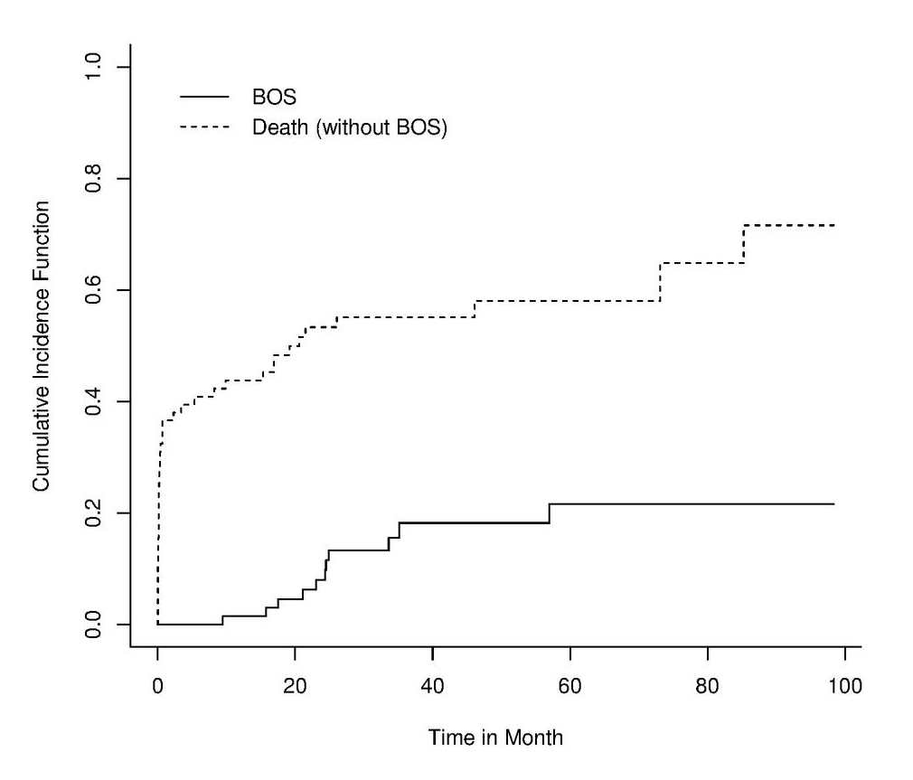
Figure 1 The estimate of the cumulative incidence function of BOS and death.

Moreover, cyclosporine is a maintenance immunosupressive regimen post-LTX, and monitoring the serum cyclosporine level (SCL) is routine and mandatory for recipients post-LTX [23]. SCL is correlated with clinical outcomes in transplant [24]. In this sample, the recipient’s SCL was measured starting from intensive care unit and during the patient’s follow-ups. The minimum and maximum of longitudinal measurements were 10 and 60, respectively. The aim of this study was to evaluate the association between SCL and BOS as well as the association between SCL and death controlling for sex, age at LTX, type of transplant, cytomegalovirus (CMV) infection, history of acute rejection (AR), and body mass index (BMI). The estimate of the cumulative incidence function of BOS and death is shown in Figure 1. In addition, Figure 2 illustrates the profile plot for the patients with SCL and the corresponding smooth curve.

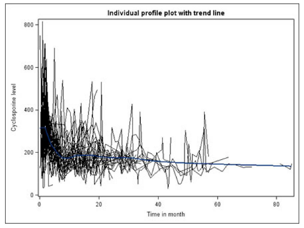
Figure 2 Profile plot for the patients with SCLs along with smooth curve.

3 Proposed Model

Assume there are $n$ subjects. Suppose $Y_i(t)$ is the longitudinal measurements for the $ith$ subject observed at time $t\in \{a_{i1},a_{i2},\mathrm{\dots },a_{i{n}_i}\}$, where $n_i\ge 1$. Let $t_i$ and ${\delta }_i$ denote the competing risks data presenting failure/censor time and indicator, respectively. ${\delta }_i$ takes three possible values 0, 1, and 2, corresponding to censored, failure due to cause 1, and failure due to cause 2, respectively. Throughout the paper, two competing risks are considered and their sub-distribution hazard functions are fully-specified [5]. The mechanism of censoring and competing risks times is assumed independent.

3.1 Longitudinal Submodel of the Proposed Model

Let $Y_{i1},Y_{i2},\mathrm{\dots },Y_{i{n}_i}$ be the values of longitudinal measurements, $Y_i(t)$, observed at $t\in \{a_{i1},a_{i2},\mathrm{\dots },a_{i{n}_i}\}$, i.e., $Y_{ij}=Y_i(a_{ij})$ for $j=1,\mathrm{\dots },n_i$. Although it is possible that a patient do not have any longitudinal measurement. Assume $Y_i={(Y_{i1},Y_{i2},\mathrm{\dots },Y_{i{n}_i})}^{\prime }$ for individuals with longitudinal measurements follows linear mixed effects model as follows

$$Y_i(t)={𝜶}^{\prime }{𝒙}_i+{𝒃}_i^{\prime }𝒈(t)+{ϵ}_i(t),$$

(1)

where ${𝒙}_i$ and $𝜶$ are covariates and their coefficients, respectively. $g(t)$ is a function of trajectory, and ${𝒃}_i\sim N(\mathrm{𝟎},\mathrm{\Omega })$ is a vector of subject-specific effects. It is further assumed that ${ϵ}_i\sim N_q(0,{\sigma }^2)$. The likelihood for longitudinal measurements for $ith$ subject is as follows

$L(𝜶,{\sigma }^2|Y_i,{𝒙}_i,{𝒃}_i)\propto {\displaystyle \prod _{j=1}^{n_i}}{({\sigma }^2)}^{-\frac{1}{2}}\exp \left\{-{\displaystyle \frac{1}{2{\sigma }^2}}{(Y_{ij}-{𝜶}^{\prime }{𝒙}_i-{𝒃}_i^{\prime }𝒈(t))}^2\right\}$

(2)

Note that the density function of ${𝒃}_i$ is given by

$f({𝒃}_i|\mathrm{\Omega })\propto {\left|\mathrm{\Omega }\right|}^{-1/2}\exp \left(-{\displaystyle \frac{1}{2}}{𝒃}_i^{\prime }{\mathrm{\Omega }}^{-1}{𝒃}_i\right)$

(3)

where $\mathrm{\Omega }$ is a $q\times q$ positive definite matrix.

3.2 Competing Risks Submodel of the Proposed Model

The competing risks model is a FS hazard functions as follows

$${\lambda }_k(t|{\lambda }_{k0},{𝜷}_k,{\gamma }_k,{𝒛}_i,{𝒃}_i,𝒈)={\lambda }_{k0}(t)\exp \{{𝜷}_k^{\prime }{𝒛}_i+h_k({𝒃}_i,𝒈,{\gamma }_k)\}$$

(4)

where ${\lambda }_k(t|{\lambda }_{k0},{𝜷}_k,{\gamma }_k,{𝒛}_i,{𝒃}_i,𝒈$), $k=1,2$, is the hazard functions for failure due to cause $k$. ${𝒛}_i$ is a vector of fixed covariates and ${𝜷}_k$ is the corresponding coefficient. In addition, ${\lambda }_{k0}$ is the baseline hazard function, $h(.)$ is a linear function of ${𝒃}_i$, $𝒈(t)$, ${\gamma }_k$. For example, ${𝒃}_i^{\prime }𝒈=(b_{i0},b_{i1}){(1,t)}^{\prime }=b_{i0}+b_{i1}t$ and $h_k({𝒃}_i,{𝒈}_i,{\gamma }_k)={\gamma }_k(b_{i0}+b_{i1}t)$. In the FS model, $F_1(t)=Pr(T_1<t_i,\delta =1)$ and $M_2(t)=Pr(T_2<t_i|\delta =2)Pr(\delta =2)$ are defined under the proportional hazard assumption such that

$F_1(t)=1-\exp \{-{\mathrm{\Lambda }}_1(t|{\lambda }_{10},{𝜷}_1,{\gamma }_1,{𝒛}_i,{𝒃}_i,𝒈)\}$

and

$M_2(t)=1-\exp \{-{\mathrm{\Lambda }}_2(t|{\lambda }_{20},{𝜷}_2,{\gamma }_2,{𝒛}_i,{𝒃}_i,𝒈)\}$

(5)

where

$${\mathrm{\Lambda }}_k(t|{\lambda }_{k0},{𝜷}_k,{\gamma }_k,{𝒛}_i,{𝒃}_i,𝒈)={\int }_0^t{\lambda }_k(u|{\lambda }_{k0},{𝜷}_k,{\gamma }_k,{𝒛}_i,{𝒃}_i,𝒈)𝑑u.$$

(6)

Moreover, $P(\delta =1)=1-P(\delta =2)=1-F_1(\mathrm{\infty })$ is assumed to overcome the non-identifiability issue ([5]). Considering $h_k({𝒃}_i,𝒈(t),{\gamma }_k)=h^{*}({𝒃}_i,{\gamma }_k)$ where $h^{*}$ is a linear function of ${𝒃}_i$ and ${𝜸}_{k2}$, the trajectory model in (4) reduces to shared parameter model. Moreover, when ${\gamma }_k=0$ then $h_k({𝒃}_i,𝒈,{\gamma }_k)\equiv \mathrm{𝟎}$ which results in fitting competing risks model to the data alone without the longitudinal model. Let ${𝜽}_1=({𝜷}_1,{\gamma }_1)$ and ${𝜽}_2=({𝜷}_2,{\gamma }_2)$. The likelihood function for competing risks model for the $ith$ subject is given by

$L({\lambda }_{10},{\lambda }_{20},{𝜽}_1,{𝜽}_2,\mathit{\varphi }|t_i,{\delta }_i,{𝒛}_i,{𝒃}_i,𝒈)$
$\mathrm{\hspace{1em}\hspace{1em}}={\left[{\lambda }_1(t_i|{\lambda }_{10},{𝜽}_1,{𝒛}_i,{𝒃}_i,𝒈)\exp \{-{\mathrm{\Lambda }}_1(t_i|{\lambda }_{10},{𝜽}_1,{𝒛}_i,{𝒃}_i,𝒈)\}\right]}^{I_{\{{\delta }_i=1\}}}$
$\mathrm{\hspace{1em}\hspace{1em}}\mathit{\hspace{1em}}[{\lambda }_2(t_i|{\lambda }_{20},{𝜽}_2,{𝒛}_i,{𝒃}_i,𝒈)\exp \{-{\mathrm{\Lambda }}_2(t_i|{\lambda }_{20},{𝜽}_2,{𝒛}_i,{𝒃}_i,𝒈)$
$\mathrm{\hspace{1em}\hspace{1em}}\mathit{\hspace{1em}}-{\mathrm{\Lambda }}_1(\mathrm{\infty }|{\lambda }_{10},{𝜽}_1,{𝒛}_i,{𝒃}_i,𝒈)\}]{}^{I_{\{{\delta }_i=2\}}}$
$\mathrm{\hspace{1em}\hspace{1em}}\mathit{\hspace{1em}}[\exp \{-{\mathrm{\Lambda }}_1(t_i|{\lambda }_{10},{𝜽}_1,{𝒛}_i,{𝒃}_i,𝒈)\}$
$\mathrm{\hspace{1em}\hspace{1em}}\mathit{\hspace{1em}}-(1-\exp \{-{\mathrm{\Lambda }}_2(t_i|{\lambda }_{20},{𝜽}_2,{𝒛}_i,{𝒃}_i,𝒈)\})$
$\mathrm{\hspace{1em}\hspace{1em}}\mathit{\hspace{1em}}\exp \{-{\mathrm{\Lambda }}_1(\mathrm{\infty }|{\lambda }_{10},{𝜽}_1,{𝒛}_i,{𝒃}_i,𝒈)\}]{}^{I_{\{{\delta }_i=0\}}}$	(7)

3.3 The Likelihood Function

The longitudinal measurements which are caused by any reason assumed missing at random under the other cause. Write $𝜽=(𝜶,{\sigma }^2,\mathrm{\Omega },{\lambda }_{10},{\lambda }_{20},{𝜷}_1,{𝜷}_2,{\gamma }_1,{\gamma }_2)$ as the parameter vector and $D_{obs}=(Y,𝒙,t,\delta )$ as the observed data. Using (2), (3), and (5) the likelihood function for the observed data, $L(𝜽|D_{obs})$, is considered in as follows

$L(𝜽,{𝒃}_i,𝒈|D_{obs})$	$={\displaystyle \prod _i}{\displaystyle \int L({\lambda }_{10},{\lambda }_{20},{𝜽}_1,{𝜽}_2|t_i,{\delta }_i,{𝒛}_i,{𝒃}_i,𝒈)}$
	$\mathrm{\hspace{1em}\hspace{1em}}L(𝜶,{\sigma }^2|Y_i,{𝒙}_i,{𝒃}_i)f({𝒃}_i|\mathrm{\Omega })d{𝒃}_i$	(8)

3.4 Priors and Posteriors

We consider independent normal priors for $𝜶\sim N_{p_1}(\mathrm{𝟎},c_{01}{I}_{p_1})$, ${𝜷}_1\sim N_{p_2}(\mathrm{𝟎},c_{02}{I}_{p_2})$, ${𝜷}_2\sim N_{p_3}(\mathrm{𝟎},c_{03}{I}_{p_3})$, ${\gamma }_1\sim N(0,c_{04})$, ${\gamma }_2\sim N(0,c_{05})$. In addition, ${\sigma }^2\sim I\mathrm{\Gamma }(a,b),a,b>0$, $\mathrm{\Omega }$ follows inverse wishart distribution, $\mathrm{\Omega }|V\sim I{W}_q(V,n)$, where $V\in R^{q\times q}$ is a positive definite scale matrix. Assume piecewise constant hazard model for ${\lambda }_{k0}(t)$ of the form of (9) such that $0=s_{k0}<s_{k1}<\mathrm{\dots }<s_{k{J}_k}<\mathrm{\infty }$ is a finite partition of size of $J_k+1$ on time axis.

$$\{\begin{array}{cc}{\lambda }_{10}(t)={\lambda }_{1j},\hfill & s_{1j-1}<t\le s_{1j},j=1,2,\mathrm{\dots },J_1;\hfill \\ {\lambda }_{10}(t)={\lambda }_{1J_1+1}\exp \{-(t-s_{1J_1})\},\hfill & t>s_{1J_1};\hfill \\ {\lambda }_{20}(t)={\lambda }_{2j},\hfill & s_{2j-1}<t\le s_{2j},j=1,2,\mathrm{\dots },J_2;\hfill \\ {\lambda }_{20}(t)={\lambda }_{2J_2+1},\hfill & t>s_{2J_2}.\hfill \end{array}$$

(9)

Let ${𝝀}_1=({\lambda }_{1j}),j=1,\mathrm{\dots },J_1+1$, ${𝝀}_2=({\lambda }_{2j}),j=1,\mathrm{\dots },J_2+1$ and ${\lambda }_{kj}$ follows independent gamma prior ${\lambda }_{kj}\sim \mathrm{\Gamma }(a_{kj},b_{kj}),a_{kj},b_{kj}>0$ for $k=1,2$. Further, we assume that all the parameters are independent $\pi (𝜽)=\pi (𝜶)\pi ({\sigma }^2)\pi ({\mathrm{\Omega }}^{-1}|V)\pi ({𝝀}_1)\pi ({𝝀}_2)\pi ({𝜷}_1)\pi ({𝜷}_2)\pi ({\gamma }_1)\pi ({\gamma }_2)$. Then, the posterior distribution is given by

$\pi (𝜽|D_{obs})\propto L(𝜽|D_{obs})\times \pi (𝜽)$

(10)

3.5 Computational Development

We adopt Markov Chain Monte Carlo (MCMC) paradigm; Metropolis Hastings algorithm and efficient Gibbs sampling algorithm to sample from the joint posterior distribution in (10) through steps: First, we sample from $f({𝒃}_i|\mathrm{\Omega })$ using Metropolis Hastings algorithm for censored subjects. Second, we used complete data likelihood for FS model through definition of two latent variables ${\eta }_i$ and $u_i$ avoiding complexity form in the censor part of the likelihood. Let $\eta =({\eta }_i:{\delta }_i=0,1\le i\le n)$ and $u=(u_i:{\delta }_i=0,{\eta }_i=1,1\le i\le n)$ such that $u_i\ge t_i$. Then, the augmented likelihood for the censored part is given by

${\left[{\lambda }_1(u_i|{\lambda }_{10},{𝜽}_1,{𝒛}_i,{𝒃}_i,𝒈)\exp \{-{\mathrm{\Lambda }}_1(u_i|{\lambda }_{10},{𝜽}_1,{𝒛}_i,{𝒃}_i,𝒈)\}\right]}^{I_{\{{\delta }_i=0,{\eta }_i=1\}}}$
$\mathrm{\hspace{1em}\hspace{1em}}\times [\exp \{-{\mathrm{\Lambda }}_2(t_i|{\lambda }_{20},{𝜽}_2,{𝒛}_i,{𝒃}_i,𝒈)$
$\mathrm{\hspace{1em}\hspace{1em}}-{\mathrm{\Lambda }}_1(\mathrm{\infty }|{\lambda }_{10},{𝜽}_1,{𝒛}_i,{𝒃}_i,𝒈)\}]{}^{I_{\{{\delta }_i=0,{\eta }_i=2\}}}$	(11)

It can be shown that ${\sum }_{𝜼}\int \int \pi (𝜽,𝜼,𝒖,𝒃|D_{obs})𝑑𝒖𝑑𝒃=\pi (𝜽|D_{obs})$. For detail see [5]. The sampling algorithm requires sampling from the full conditional posterior densities which are shown in Appendix 1 elaborately.

4 Simulation Study

In this section, a simulation study is carried out to check different scenarios under the proposed model. For the longitudinal submodel, covariates $x_{i1}$ and $x_{i2}$ are generated from $Gaussian(2,1)$ and $Bernouli(0.2)$, respectively, with true parameters ${𝒃}_l={(b_{l0},b_{l1},b_{l2},b_{l3})}^{\prime }$. The linear mixed effect model including random intercept $b_{0i}$ is as follows:

$$Y(t_{ij})=b_{l0}+b_{l1}{t}_{ij}+b_{l2}{x}_{i1}+b_{l3}{x}_{i2}+b_{0i}+ϵ(t_{ij})$$

where $b_{0i}\sim N(0,\sigma _b{}^2=1)$ and $ϵ(t_{ij})\sim N(0,\sigma _{ϵ}{}^2=1)$ are mutually independent. It is considered 25 time points for the longitudinal measurements such that $a_{i1}=0$ and $Y_{i1}$ is the baseline longitudinal measurement. For the competing risks submodel, we assumes two causes where cause 1 is the event of interest and $p(\delta =1)\simeq 1/3$. Covariates $z_{i1}$ and $z_{i2}$ given $z_{i1}$ are generated from $N(0,1)$ and $Bernouli(p(z_{i1}))$ where $p(z_{i1})=\frac{exp(0.3+.2z_{i1})}{1+exp(0.3+.2z_{i1})}$, respectively. Two covariates with true parameters ${𝜷}_1={({\beta }_{11},{\beta }_{12})}^{\prime }$ and ${𝜷}_2={({\beta }_{21},{\beta }_{22})}^{\prime }$ are considered. The failure times of two causes follow distinct piecewise exponential distributions such that partitioned time axis is as follows; $s_{1j}=(0,3,6,9)$ with corresponding ${𝝀}_1=(0.02,0.08,0.1,0.15)$ and $s_{2j}=(0,5,10,15,20,25)$ with corresponding ${𝝀}_2=(0.05,0.10,0.15,0.20,0.25)$. For more details about FS model simulation see [5]. ${\lambda }_1(t_i)$ and ${\lambda }_2(t_i)$ are hazard functions for the competing risks involving shared random intercept $b_{0i}$.

${\lambda }_1(t_i)={\lambda }_{01}(t_i)\exp \{{\beta }_{11}{z}_{i1}+{\beta }_{12}{z}_{i2}+{\gamma }_1{b}_{0i}\}$
${\lambda }_2(t_i)={\lambda }_{02}(t_i)\exp \{{\beta }_{21}{z}_{i1}+{\beta }_{22}{z}_{i2}+{\gamma }_2{b}_{0i}\}$	(12)

300 data sets with the sample size (N) of 75, 100, 300, 500, and 800 were generated. The true value, estimate, standard deviation (SD), coverage probability (CP), and mean square error (MSE) of each parameter for both submodels are given in Table 1. Squared error loss, the most commonly used loss function, was used for the estimations of the parameters. The higher sample size, the more acceptable CP. For sample size of 800, all the CPs are around 0.95. The simulation study showed that MSE and CP increased as the sample size increased. However, parameter’s bias has no decreasing trend when sample size increased.

Table 1 The true value, estimate (SD), bias, MSE, and CP for the simulated joint model using Bayesian approach

	Real value	2	3	-2	1	1	0.1	0.3	0.8	0.1	0.9	1	0.5	0.5	1
N	Parameter	$b_{l0}$	$b_{l1}$	$b_{l2}$	$b_{l3}$	${\sigma }_e^2$	${\beta }_{11}$	${\beta }_{12}$	${\gamma }_{11}$	${\gamma }_{12}$	${\beta }_{21}$	${\beta }_{22}$	${\gamma }_{21}$	${\gamma }_{22}$	${\sigma }_b^2$
50	Estimate	1.958	3.012	-1.988	0.997	1.003	0.096	0.074	0.839	0.137	1.219	1.404	-5.149	0.882	1.111
	SD	0.552	0.605	0.238	0.062	0.066	0.284	0.586	0.556	0.646	1.189	1.875	17.296	1.811	0.372
	Bias	-0.042	0.012	0.012	-0.003	0.003	-0.004	-0.226	0.039	0.037	0.319	0.404	-5.649	0.382	0.111
	MSE	0.306	0.367	0.057	0.004	0.004	0.080	0.394	0.310	0.419	1.515	3.680	331.048	3.426	0.151
	CP	0.897	0.927	0.897	0.933	0.930	0.913	0.870	0.900	0.873	0.837	0.857	0.873	0.823	0.927
75	Estimate	1.995	2.991	-1.999	1.004	1.003	0.089	0.129	0.807	0.143	1.049	1.184	-3.513	0.666	1.064
	SD	0.431	0.497	0.183	0.051	0.052	0.192	0.420	0.458	0.365	0.490	0.982	15.192	0.859	0.275
	Bias	-0.005	-0.009	0.001	0.004	0.003	-0.011	-0.171	0.007	0.043	0.149	0.184	-4.013	0.166	0.064
	MSE	0.186	0.247	0.034	0.003	0.003	0.037	0.205	0.210	0.135	0.262	0.998	246.917	0.765	0.080
	CP	0.913	0.920	0.913	0.953	0.930	0.920	0.897	0.920	0.910	0.917	0.907	0.867	0.877	0.947
100	Estimate	2.012	3.011	-2.005	1.000	1.001	0.109	0.195	0.854	0.077	0.932	1.000	-1.635	0.583	1.035
	SD	0.380	0.392	0.159	0.043	0.048	0.167	0.331	0.352	0.290	0.370	0.659	11.680	0.512	0.232
	Bias	0.012	0.011	-0.005	0.000	0.001	0.009	-0.105	0.054	-0.023	0.032	0.000	-2.135	0.083	0.035
	MSE	0.145	0.154	0.025	0.002	0.002	0.028	0.121	0.127	0.084	0.138	0.434	140.976	0.269	0.055
	CP	0.917	0.927	0.923	0.953	0.930	0.923	0.933	0.920	0.900	0.910	0.930	0.900	0.930	0.949
300	Estimate	2.003	2.991	-1.999	1.002	1.002	0.106	0.243	0.788	0.093	0.866	0.930	0.398	0.500	1.012
	SD	0.197	0.218	0.086	0.024	0.026	0.084	0.180	0.189	0.133	0.167	0.303	0.455	0.206	0.119
	Bias	0.003	-0.009	0.001	0.002	0.002	0.006	-0.057	-0.012	-0.007	-0.034	-0.070	-0.102	0.000	0.012
	MSE	0.039	0.048	0.007	0.001	0.001	0.007	0.036	0.036	0.018	0.029	0.097	0.218	0.042	0.014
	CP	0.933	0.933	0.927	0.943	0.943	0.943	0.930	0.940	0.943	0.937	0.937	0.927	0.940	0.973
500	Estimate	2.002	3.005	-2.001	1.000	1.002	0.101	0.272	0.795	0.102	0.818	0.906	0.372	0.463	1.023
	SD	0.149	0.152	0.066	0.019	0.020	0.062	0.137	0.157	0.096	0.126	0.233	0.331	0.143	0.094
	Bias	0.002	0.005	-0.001	0.000	0.002	0.001	-0.028	-0.005	0.002	-0.082	-0.094	-0.128	-0.037	0.023
	MSE	0.022	0.023	0.004	0.000	0.000	0.004	0.020	0.025	0.009	0.023	0.063	0.126	0.022	0.009
	CP	0.933	0.948	0.940	0.963	0.943	0.950	0.947	0.940	0.943	0.935	0.927	0.923	0.937	0.953
800	Estimate	2.010	3.003	-2.006	0.999	1.000	0.096	0.296	0.786	0.098	0.826	0.893	0.390	0.464	1.009
	SD	0.122	0.129	0.051	0.016	0.015	0.055	0.112	0.111	0.078	0.092	0.177	0.265	0.116	0.076
	Bias	0.010	0.003	-0.006	-0.001	0.000	-0.004	-0.004	-0.014	-0.002	-0.074	-0.107	-0.110	-0.036	0.009
	MSE	0.015	0.017	0.003	0.000	0.000	0.003	0.013	0.013	0.006	0.014	0.043	0.082	0.015	0.006
	CP	0.937	0.963	0.947	0.963	0.947	0.957	0.960	0.943	0.950	0.952	0.945	0.940	0.955	0.953

5 Lung Transplant Study

Table 2 describes the recipient’s characteristics. The mean and the median of longitudinal measurement time points were 28 and 26, respectively. It was considered random intercept model for recipient $i$ at time point $j$,

$SCL(t_{ij})$	$=b_{l0}+b_{l1}{t}_{ij(0,10]}+b_{l2}{t}_{ij(0,10]}^2+{\beta }_{l3}{t}_{ij(10,\mathrm{\infty })}+b_{0i}+ϵ(t_{ij})$
${\lambda }_{BOS}(t_i)$	$={\lambda }_{0BOS}(t_i)\exp \{{\beta }_{11}Se{x}_i+{\beta }_{12}Ag{e}_i+{\beta }_{13}Typ{e}_i$
	$\mathrm{\hspace{1em}}+{\beta }_{14}CM{V}_i+{\beta }_{15}A{R}_i+{\beta }_{16}BM{I}_i+{\gamma }_1{b}_{0i}\}$
${\lambda }_{Death}(t)$	$={\lambda }_{0Death}(t_i)\exp \{{\beta }_{21}Se{x}_i+{\beta }_{22}Ag{e}_i+{\beta }_{23}Typ{e}_i$
	$\mathrm{\hspace{1em}}+{\beta }_{24}CM{V}_i+{\beta }_{25}A{R}_i+{\beta }_{26}BM{I}_i+{\gamma }_2{b}_{0i}\}$	(13)

where $b_{0i}\sim N(0,{\sigma }_b^2)$ and $ϵ(t_{ij})\sim N(0,{\sigma }_e^2)$ are mutually independent. Table 2 shows the results of the joint model in (13). The first part of the Table 2 shows the estimates (SE) and 95% credible set (CS) for the longitudinal submodel, and the second and the third parts present the estimates (SE) along with 95% CS, and Hazard ratio (HR) accompanied by 95% CS, respectively. The results shows that SCL follows a quadratic pattern up to 10 months post-LTX and a linear form afterwards. The risk of BOS was 3.1 (95% CS:1.5,14.8) times higher in recipients who experienced AR compared to recipients with no history of AR . In addition, recipients who had history of CMV infection and higher BMI had a significantly higher risk of death. The estimates revealed that SCL was associated with higher risk of death significantly. The higher initial SCL was associated with higher risk of death (95% CS: (-0.07, -0.008)). However, the initial SCL was not related to BOS risk significantly (95% CS: (-0.02, 0.012)) controlling for SCL and other covariates.

Table 2 The recipient’s characteristics

Variable	Mean (SE) or N (%)
Age	35.87 (13.2)
BMI	19.98 (3.94)
Sex (female)	15 (21)
AR (Grade II and higher) $(+)$	12 (17)
CMV $(+)$	22 (31)
Type of transplant (lateral)	33 (46.5)

6 Discussion

Joint modeling has been developed for more than one causes of failure to assess the relationship between longitudinal measurements and causes as well as providing a tool for inferences of longitudinal measurements at the presence of non-informative censoring.

Table 3 The results of the proposed joint model on LTX data using Bayesian approach

Submodel	Term in the Model	Estimation (95% Credible Set)
Longitudinal
	Intercept	130 (121.83, 155.09)
	$Tim{e}_{(0,10]}$	$-$85.04 ($-$94.1, $-$73.08)
	$Tim{e}_{(0,10]}^2$	12.29 (6.37, 18.76)
	$Tim{e}_{(10,\mathrm{\infty })}$	$-$29.53 ($-$39.11, $-$21.07)
Competing risks		Hazard Ratio (95% Credible Set)
BOS
(the event of interest)
	$Se{x}_{female}$	4.1 (1.15, 12.21)
	Age	0.93 (0.69, 1.35)
	$Typeoftransplan{t}_{lateral}$	1.5 (0.01, 77.21)
	$CM{V}_{+}$	2.9 (0.69, 18.28)
	$A{R}_{+}$	3.21 (1.41, 14.99)
	BMI	0.36 (0.19, 1.23)
Death
(the competing risk)
	$Se{x}_{female}$	1.53 (0.27, 13.06)
	Age	0.81 (0.78, 1.01)
	$Typeoftransplan{t}_{lateral}$	2.73 (0.56, 8.92)
	$CM{V}_{+}$	3.14 (1.47, 5.57)
	$A{R}_{+}$	1.03 (0.08, 13.89)
	BMI	1.12 (1.03, 1.73)
Association parameter
	${\gamma }_1$	$-$0.01 ($-$0.017, 0.019)
	${\gamma }_2$	$-$0.03 ($-$0.07, $-$0.009)

In this study, we proposed a new joint model for longitudinal measurements and competing risks in which FS model is utilized as the competing risks submodel. In addition, a linear mixed model was utulized for the longitudinal submodel. These two submodels are linked through a shared random effect approach [11]. The asymptotic properties of the proposed model is complex although convergency and identifiability of the model is shown throughout the simulation. Recently, Tian et. al used quantile regression for longitudinal mixed models for joint model with multiple data features. They employed Monte Carlo Expectation-Maximization algorithm for estimation problem [25]. Zhang et al proposed a joint model of mixed effects regression models for longitudinal measures and a cure rate model under the semi-competing risks framework; the disease progression as the non-terminal event, and the occurrence of death as the terminal event. The Bayesian paradigm was applied for estimation process [26].

However, other semiparametric competing risks submodels such as mixture model [11] and CSHF [12] have been used previously as the competing risks submodel in joint models. It is noteworthy that CSHF is not able to incorporate the correlation between causes however, FS model [5] takes into account the correlation between competing risks via $P(\delta =1)+P(\delta =2)=1$ to overcome nonidentifiability issue. FS model can incorporates both risks in one likelihood function and estimate all the covariate effects simultaneously.

The results of the proposed model on LTX data revealed that SCL was related to the BOS risk nonsignificantly, and SCL was negatively associated with mortality risk. Moreover, AR was hazardous factor on BOS development, and CMV infection as well as BMI were found risk factors of mortality post-LTX. Similar results were found in [27]. Hosseini-Baharanchi et al applied a joint model of initial SCL and mortality on LTX data in which it was found that AR was a predictor of mortality as well as a negative association between higher initial SCL and lower mortality risk [28].

In this study, the submodels are linked using shared random intercept only, it can be further extended to both shared random intercept and random slope.t is suggested to find a robust estimation procedures when random effects violate the normality assumption for future researches. The code is written in R 3.2.1 and is available upon the request.

7 Appendix

Full conditional posterior densities for some of the parameters including $𝜶$, ${\sigma }^2$, ${\mathrm{\Omega }}^{-1}$, ${𝜷}_1$, and ${𝝀}_1$

1. Sampling $𝜶$ from

$𝜶|{𝒃}_i,D_{obs}$	$\sim N({\left[{\displaystyle \sum _{i\in G_1}}({\displaystyle \frac{n_{i{i}_i^{\prime }}}{{\sigma }^2}}+{\displaystyle \frac{I}{c_{01}}})\right]}^{-1}$
	$\mathrm{\hspace{1em}}{\displaystyle \sum _{i\in G_1}}i{\displaystyle \sum _{j=1}^{n_j}}(Y_{ij}-{𝒃}_i^{\prime }𝒈(t)),$
	$\mathrm{\hspace{1em}}{\left[{\displaystyle \sum _{i\in G_1}}({\displaystyle \frac{n_{i{i}_i^{\prime }}}{{\sigma }^2}}+{\displaystyle \frac{I}{c_{01}}})\right]}^{-1})$	(14)

2. Sampling ${\sigma }^2$ from

${\sigma }^2|{𝒃}_i,D_{obs}\sim IG({\displaystyle \frac{n_i}{2}}+a,{\displaystyle \frac{{\sum }_{j=1}^{n_i}{(Y_{ij}-{𝜶}^{\prime }{}_i-{𝒃}_i^{\prime }𝒈(t))}^2}{2}}+b)$

3. Sampling ${\mathrm{\Omega }}^{-1}$ from

${\mathrm{\Omega }}^{-1}|{𝒃}_i,D_{obs}\sim IWishart(n+q+1,{𝒃}_i{𝒃}_i^{\prime }+V)$

4. Sampling ${𝜷}_1$ from

$\pi ({𝜷}_1|{𝒃}_i,{\eta }_i,u_i,{𝝀}_1,{𝝀}_2,{\gamma }_{11},{𝜸}_{12},D_{obs})$

$\mathrm{\hspace{1em}\hspace{1em}}\propto {\displaystyle \prod _{i=1}^n}[{\lambda }_{10}(t_i)\exp \{{𝜷}_1^{\prime }{𝒛}_i+{\gamma }_{11}(1-d_i)+d_i{h}_1({𝒃}_i,𝒈(t),{𝜸}_{12})\}$

$\mathrm{\hspace{1em}\hspace{1em}}\mathit{\hspace{1em}}\exp \{{\displaystyle {\int }_0^{t_i}}{\lambda }_{10}(u)\exp \{{𝜷}_1^{\prime }{𝒛}_i+{\gamma }_{11}(1-d_i)$

$\mathrm{\hspace{1em}\hspace{1em}}\mathit{\hspace{1em}}+d_i{h}_1({𝒃}_i,𝒈(t),{𝜸}_{12})\}du\}]{}^{I_{\{{\delta }_i=1\}}}$

$\mathrm{\hspace{1em}\hspace{1em}}\mathit{\hspace{1em}}\times [\exp \{-{\displaystyle {\int }_0^{\mathrm{\infty }}}{\lambda }_{10}(u)\exp \{{𝜷}_1^{\prime }{𝒛}_i+{\gamma }_{11}(1-d_i)$

$\mathrm{\hspace{1em}\hspace{1em}}\mathit{\hspace{1em}}+d_i{h}_1({𝒃}_i,𝒈(t),{𝜸}_{12})\}du]{}^{I_{\{{\delta }_i=2}\}}$

$\mathrm{\hspace{1em}\hspace{1em}}\mathit{\hspace{1em}}\times [{\lambda }_{10}(t_i)\exp \{{𝜷}_1^{\prime }{𝒛}_i+{\gamma }_{11}(1-d_i)+d_i{h}_1({𝒃}_i,𝒈(t),{𝜸}_{12})\}$

$\mathrm{\hspace{1em}\hspace{1em}}\mathit{\hspace{1em}}\exp \{{\displaystyle {\int }_0^{u_i}}{\lambda }_{10}(u)\exp \{{𝜷}_1^{\prime }{𝒛}_i+{\gamma }_{11}(1-d_i)$

$\mathrm{\hspace{1em}\hspace{1em}}\mathit{\hspace{1em}}+d_i{h}_1({𝒃}_i,𝒈(t),{𝜸}_{12})\}du\}]{}^{I_{\{{\delta }_i=0,{\eta }_i=1\}}}$

$\mathrm{\hspace{1em}\hspace{1em}}\mathit{\hspace{1em}}\times [\exp \{-{\displaystyle {\int }_0^{\mathrm{\infty }}}{\lambda }_{10}(u)\exp \{{𝜷}_1^{\prime }{𝒛}_i+{\gamma }_{11}(1-d_i)$

$\mathrm{\hspace{1em}\hspace{1em}}\mathit{\hspace{1em}}+d_i{h}_1({𝒃}_i,𝒈(t),{𝜸}_{12})\}du\}\left]{}^{I_{\{{\delta }_i=0,{\eta }_i=2\}}}\exp \right\{-{\displaystyle \frac{1}{2c_{02}}}{𝜷}_1^{\prime }{𝜷}_1\}$

5. Sampling ${𝝀}_1$ from

$\pi ({𝝀}_1|{𝒃}_i,{\eta }_i,u_i,{𝜷}_1,{𝜷}_2,{\gamma }_{k1},{𝜸}_{k2},D_{obs})$
$\mathrm{\hspace{1em}\hspace{1em}}\propto {\displaystyle \prod _{i=1}^n}[{\lambda }_{10}(t_i)\exp \{{𝜷}_1^{\prime }{𝒛}_i+{\gamma }_{11}(1-d_i)$
$\mathrm{\hspace{1em}\hspace{1em}}\mathit{\hspace{1em}}+d_i{h}_1({𝒃}_i,𝒈(t),{𝜸}_{12})\}$
$\mathrm{\hspace{1em}\hspace{1em}}\mathit{\hspace{1em}}\exp \{{\displaystyle {\int }_0^{t_i}}{\lambda }_{10}(u)\exp \{{𝜷}_1^{\prime }{𝒛}_i+{\gamma }_{11}(1-d_i)$
$\mathrm{\hspace{1em}\hspace{1em}}\mathit{\hspace{1em}}+d_i{h}_1({𝒃}_i,𝒈(t),{𝜸}_{12})\}du\}]{}^{I_{\{{\delta }_i=1\}}}$
$\mathrm{\hspace{1em}\hspace{1em}}\mathit{\hspace{1em}}\times [\exp \{-{\displaystyle {\int }_0^{\mathrm{\infty }}}{\lambda }_{10}(u)\exp \{{𝜷}_1^{\prime }{𝒛}_i+{\gamma }_{11}(1-d_i)$
$\mathrm{\hspace{1em}\hspace{1em}}\mathit{\hspace{1em}}+d_i{h}_1({𝒃}_i,𝒈(t),{𝜸}_{12})\}du\}]{}^{I_{\{{\delta }_i=2}\}}$
$\mathrm{\hspace{1em}\hspace{1em}}\mathit{\hspace{1em}}\times [\exp \{{\lambda }_{10}(u)\exp \{{𝜷}_1^{\prime }{𝒛}_i+{\gamma }_{11}(1-d_i)+d_i{h}_1({𝒃}_i,𝒈(t),{𝜸}_{12})\}$
$\mathrm{\hspace{1em}\hspace{1em}}\mathit{\hspace{1em}}{\displaystyle {\int }_0^{u_i}}{\lambda }_{10}(u)\exp \{{𝜷}_1^{\prime }{𝒛}_i+{\gamma }_{11}(1-d_i)$
$\mathrm{\hspace{1em}\hspace{1em}}\mathit{\hspace{1em}}+d_i{h}_1({𝒃}_i,𝒈(t),{𝜸}_{12})\}du\}]{}^{I_{\{{\delta }_i=0,{\eta }_i=1\}}}$
$\mathrm{\hspace{1em}\hspace{1em}}\mathit{\hspace{1em}}\times [\exp \{-{\displaystyle {\int }_0^{\mathrm{\infty }}}{\lambda }_{10}(u)\exp \{{𝜷}_1^{\prime }{𝒛}_i+{\gamma }_{11}(1-d_i)$
$\mathrm{\hspace{1em}\hspace{1em}}\mathit{\hspace{1em}}+d_i{h}_1({𝒃}_i,𝒈(t),{𝜸}_{12})\}du\}]{}^{I_{\{{\delta }_i=0,{\eta }_i=2\}}}$
$\mathrm{\hspace{1em}\hspace{1em}}\mathit{\hspace{1em}}{\displaystyle \prod _{j=1}^{J_1+1}}{\lambda }_{1j}^{a_{1j}-1}\exp \{-b_{kj}{\lambda }_{1j}\}$	(18)

References

[1] Prentice, R.L., Kalbfleisch, J.D., Peterson Jr, A.V., Flournoy, N., Farewell, V. and N. Breslow, The analysis of failure times in the presence of competing risks, Biometrics, 541-554, 1978.

[2] Larson M.G. and Dinse, G.E. A mixture model for the regression analysis of competing risks data, Applied statistics 16, 201-211, 1985.

[3] Gray, R.J. A class of k-sample tests for comparing the cumulative incidence of a competing risk, The Annals of statistics, 1141-1154, 1988.

[4] Fine J.P. and Gray, R.J. A proportional hazards model for the subdistribution of a competing risk, Journal of the American Statistical Association 94, 496-509, 1999.

[5] Ge M. and Chen, M.H. Bayesian inference of the fully specified subdistribution model for survival data with competing risks, Lifetime data analysis 18, 339-363, 2012.

[6] Sweeting M.J. and Thompson, S.G. Joint modelling of longitudinal and time-to-event data with application to predicting abdominal aortic aneurysm growth and rupture, Biometrical Journal 53, 750-763, 2011.

[7] Tsiatis, A.A., Degruttola, V. and Wulfsohn, M. Modeling the relationship of survival to longitudinal data measured with error: applications to survival and cd4 counts in patients with aids, Journal of the American Statistical Association 90, 27-37, 1995.

[8] De Gruttola V. and Tu, X.M. Modelling progression of cd4-lymphocyte count and its relationship to survival time, Biometrics 1003-1014, 1994.

[9] Ibrahim, J.G., Chen, M.H., and Sinha, D. Bayesian survival analysis, Wiley Online Library, 2005.

[10] Tsiatis A.A. and Davidian, M. Joint modeling of longitudinal and time-to-event data: an overview, Statistica Sinica 14, 809-834, 2004.

[11] Elashoff, R.M., Li, G. and Li, N. An approach to joint analysis of longitudinal measurements and competing risks failure time data, Statistics in medicine 26, 2813-2835, 2007.

[12] Elashoff, R.M., Li, G. and Li, N. A joint model for longitudinal measurements and survival data in the presence of multiple failure types, Biometrics 64, 762-771, 2008.

[13] Baghfalaki, T., Ganjali, M. and Hashemi, R. Bayesian joint modeling of longitudinal measurements and time-to-event data using robust distributions, Journal of biopharmaceutical statistics 24, 834-855, 2014.

[14] Baghfalaki, T., Ganjali, M. and Berridge, D. Joint modeling of multivariate longitudinal mixed measurements and time to event data using a bayesian approach, Journal of Applied Statistics 41, 1934-1955, 2014.

[15] Ganjali M. and Baghfalaki, T. A copula approach to joint modeling of longitudinal measurements and survival times using monte carlo expectation-maximization with application to aids studies, Journal of biopharmaceutical statistics 25, 1077-1099, 2015.

[16] Baghfalaki, T., Ganjali, M. and Verbeke, G. A shared parameter model of longitudinal measurements and survival time with heterogeneous random-effects distribution, Journal of Applied Statistics 44, 2813-2836, 2017.

[17] Li, N., Elashoff, R.M. and Li, G. Robust joint modeling of longitudinal measurements and competing risks failure time data, Biometrical Journal 51, 19-30, 2009.

[18] Li, N., Elashoff, R.M., Li, G. and Saver, J. Joint modeling of longitudinal ordinal data and competing risks survival times and analysis of the ninds rt-pa stroke trial, Statistics in medicine 29, 546-557, 2010.

[19] Hu C. and Tsodikov, A. Joint modeling approach for semicompeting risks data with missing nonterminal event status, Lifetime data analysis 20,563-83, 2009.

[20] Huang, X., Li, G., Elashoff, R.M. and Pan, J. A general joint model for longitudinal measurements and competing risks survival data with heterogeneous random effects, Lifetime data analysis 17, 80-100, 2011.

[21] Burton, C.M., Carlsen, J., Mortensen, J. Andersen, C.B., Milman, N. and Iversen, M. Longterm survival after lung transplantation depends on development and severity of bronchiolitis obliterans syndrome, The Journal of heart and lung transplantation 26, 681-686, 2007.

[22] Stehlik, J., Edwards, L.B. , Kucheryavaya, A.Y., Aurora, P., Christie, J.D., Kirk, R., Dobbels, F., Rahmel, A.O. and Hertz, M.I. The registry of the international society for heart and lung transplantation: twenty-seventh official adult heart transplant report 2010, The Journal of Heart and Lung Transplantation 29, 1089-1103, 2010.

[23] Flechner, S.M. , Kobashigawa, J. and Klintmalm, G. Calcineurin inhibitor-sparing regimens in solid organ transplantation: focus on improving renal function and nephrotoxicity, Clinical transplantation 22, 1-15, 2008.

[24] Nemati, E., Einollahi, B., Taheri, S. , Moghani-Lankarani, M., Kalantar, E., Simforoosh, N., Nafar, M. and Saadat, A. Cyclosporine trough (C0) and 2-hour postdose (C2) levels: which one is a predictor of graft loss?, Transplantation proceedings, 39, 1223-1224, 2007.

[25] Zhang F., Chen M.H., Cong X.J., Chen Q. Assessing importance of biomarkers: A Bayesian joint modelling approach of longitudinal and survival data with semi-competing risks. Statistical Modelling. 2020.

[26] Tian Y., Wang L., Tang M., Tian M. Likelihood-based quantile mixed effects models for longitudinal data with multiple features via MCEM algorithm. Communications in Statistics-Simulation and Computation. 49, 2, 2020.

[27] Hosseini-Baharanchi, F.S., Hajizadeh, E., Baghestani, A.R., Najafizadeh, K. and Shafaghi, S. Bronchiolitis obliterans syndrome and death in iranian lung transplant recipients: A bayesian competing risks analysis, Tanaffos 15, 141, 2016.

[28] Hosseini-Baharanchi, F.S., Hajizadeh, E., Baghestani, A. and Najafzadeh, K. The relationship between mortality of lung transplant recipients and serum cyclosporine levels: Joint modeling of time-to-event data and longitudinal data, International journal of organ transplantation medicine 8, 157, 2017.

Biographies

F. S. Hosseini-Baharanchi received her B.Sc. degree in Statistics and M.Sc. degree in Biostatistics from Tehran University of Medical Sciences; and Ph.D. degree in Biostatistics in 2016 from Tarbiat Modares University, Iran. Fatemeh was a visiting scholar in University of Connecticut, USA 2015. She is working in Iran University of Medical Sciences, Iran as an assistant professor in Biostatistics department since 2016. She is experienced in statistical modeling especially survival modeling and joint modeling of survival data and longitudinal measurements, especially in medical area. In addition, Fatemeh, as a member of international federation of Inventors Association, Geneva, Switzerland, helps students to pass the process of idea-to-patent as well as inventors to protect their intellectual property. She’s been focused on personal development, personal branding and innovative business models generation since 2018.

A. R. Baghestani received his B.Sc. degree in Statistics from Shahid Beheshti University and M.Sc. degree in Statistics from Tehran University of Medical Sciences; and Ph.D. degree in Biostatistics in 2010 from Tarbiat Modares University, Iran. He is associate professor in Biostatistics department in Shahid Beheshti University of Medical Sciences, Iran since 2011. He is fully-experienced in survival modeling, joint modeling, defective distributions, and competing risks analysis.

T. Baghfalaki completed his Master’s degree and Ph.D. from Shahid Beheshti University, Tehran, Iran in Statistics. She has more than 15 years of research experience. She is presently an Assistant Professor of Statistics at Tarbiat Modares University.

E. Hajizadeh received his Master’s degree in Statistics and his Ph.D. in Biostatistics from India in 1990. He is working in area of Statistics; education and research in the national and international level since 1990. He is a full Professor in Tarbiat Modares University. His area of expertise is survival analysis, competing risks data analysis, advanced linear modeling in national and international researches (including United Nations) in the field of medical and environmental topics.

K. Najafizadeh is a Pulmonary Disease Specialist who established the Lung transplant program in 2000 in Iran. In 2004 she also established organ donation program in one of the main Universities of Tehran to increase the rate of organ donation for patients on transplant waiting lists especially on the list of lung transplant which was her main concern. She performed some projects for increasing the donation rate in this University and could get the family consent rate of 96% and make a PMP of 32.4 in its area with 10 million population with her colleagues. Katayoun was assigned the Director of Organ donation and Transplantation Office of the Ministry of Health of Iran in 2014. Again her colleagues and she presented some projects to the Minister of Health and with his approval and Iranian Supreme Transplant Council confirmation they started these projects in the country and could increase the organ donation rate in Iran significantly. She also with the best of Iranian Transplant and also Culture and Art experts of Iran established a NGO named “Iranian Society of Organ Donation” to help the Ministry of Health Transplant Management Center especially in issues like Social awareness activities, Donor family support, Donor teams education, research and every other related activities which is needed to improve organ donation and transplantation in Iran. In 2018 responsibility of establishing “Organ donation and Transplantation Registry of Iran” (OTRI), “Organ Transfer System of Iran” (OTSI), Quality assurance and audit of organ procurement units and some other important projects of the Ministry of Health has been passed to ISOD and she with her colleagues in their NGO are hardly working on these important issues. She has been a member of ISODP council since 2017.

S. Shafaghi is a MD., PhD. She was lung transplant coordinator and responsible for pre and post lung transplantation follow up for 5 years till 2015. She established ex-vivo lung perfusion program in Iran in 2016 as her PhD thesis in order to increase the rate of lung donation for patients on long transplant waiting list. Then she was in charge of organ allocation in Iranian Ministry of Health and Medical Education from 2015 to 2018. She has dramatic role for establishing computerized organized national organ donation and transplantation registry in Iran. In 2018 responsibility of research committee of “Organ donation and Transplantation Registry of Iran” (OTRI) project has been passed to her. She was assigned the researcher of cardiovascular diseases department in lung transplantation research unit of national research institute of tuberculosis and lung disease (NRITLD) of Shahid Beheshti University of Medical Sciences, Tehran, Iran.

Journal of Reliability and Statistical Studies, Vol. 13_2-4, 221–242.
doi: 10.13052/jrss0974-8024.13241
© 2020 River Publishers

Abstract

1 Introduction

2 The Motivating Lung Transplant Data

3 Proposed Model

3.1 Longitudinal Submodel of the Proposed Model

3.2 Competing Risks Submodel of the Proposed Model

3.3 The Likelihood Function

3.4 Priors and Posteriors

3.5 Computational Development

4 Simulation Study

5 Lung Transplant Study

6 Discussion

7 Appendix

References

Biographies