Prediction of Area and Production of Groundnut Using Box-Jenkins Arima and Neural Network Approach

S. T. Pavana Kumar^* and Ferdinand B. Lyngdoh

College of Community Science, Central Agricultural University, Tura, Meghalaya-794005, India

E-mail: pvnkmr625@gmail.com

*Corresponding Author

Received 12 July 2020; Accepted 23 October 2020; Publication 29 December 2020

Abstract

Selection of parameters for Auto Regressive Integrated Moving Average (ARIMA) model in the prediction process is one of the most important tasks. In the present study, groundnut data was utlised to decide appropriate $p$, $d$, $q$ parameters for ARIMA model for the prediction purpose. Firstly, the models were fit to data without splitting into training and validation/testing sets and evaluated for their efficiency in predicting the area and production of groundnut over the years. Meanwhile, models are compared among other fitted ARIMA models with different p, d, q parameters based on decision criteria’s viz., ME, RMSE, MAPE, AIC, BIC and R-Square. The ARIMA model with parameters p-2 d-1-2, q-1-2 are found adequate in predicting the area as well as production of groundnut. The model ARIMA (2, 2, 2) and ARIMA (2,1,1) predicted the area of groundnut crop with minimum error estimates and residual characteristics (e${}_{\mathrm{i}}$). The models were fit into split data i.e., training and test data set, but these models’ prediction power (R-Square) declined during testing. In case of predicting the area, ARIMA (2,2,2) was consistent over the split data but it was not consistent while predicting the production over years. Feed-forward neural networks with single hidden layer were fit to complete, training and split data. The neural network models provided better estimates compared to Box-Jenkins ARIMA models. The data was analysed using R-Studio.

Keywords: Groundnut data, Box-Jenkins models, neural network, model accuracy, parameters.

Introduction

Prediction of agricultural phenomenon has proved to be helpful for farmers and decision makers across the world. It has further helped to understand prevailing market situation, production [12, 21, 28, 9], price behavior [7, 11] and possible pests and disease attack if meteorological variables are changed suddenly. Moreover, Indian agriculture has massive land holding over wide variety of climate and potential to produce sufficient agricultural produce. As a result, many researchers have tried to predict and forecast many agricultural phenomenon [3] like prediction of rainfall, prices [16] of different agriculture produce across markets and area, production of different crops over the years using sophisticated statistical methodology. In most of the cases, authenticity of the data is a big question and the data obtained must be analyzed properly. On many instances, obtaining the auxiliary variables is difficult, therefore, time series models have become popular in the prediction process.

Groundnut is an oil seed crop, which is grown widely in the country, and approximately 80% of groundnut is produced in the rainfed condition. Mainly, state includes Andhra Pradesh, Gujarat, Karnataka, Maharashtra and Tamil Nadu, were contributing nearly 90 per cent of total production of groundnut in the country. Among all the meteorological factors, rainfall plays a deciding role in the production as well as the incidence of pests and disease can cause significant damage to the production of groundnut in the country. Unlike weather factors even the prices of agriculture commodities are volatile in nature and the groundnut prices also behaves in an unusual pattern.

A time series model has wide variety of application includes risk management [17], tourism forecasting [4] and in the medicine and pharmaceuticals sectors [13, 15, 20]. In agriculture and allied sciences, time series models are used for forecasting milk production, milk yield of certain breeds of cows, yield of a crop, prices, production, and productivity [27, 25]. These models can play a significant role in stock market decision-making [22]; its application in financial aspects like credit and banking sectors is also crucial [24].

Accurate prediction of area and production of groundnut in India will help the farming community to understand and decide the crop mix grown in a particular season, and help the decision makers. In the present study, groundnut area and production data are used to build ARIMA models, and the best ARIMA model is compared with feed-forward neural networks. The main aim of the study is to identify p, d, q parameters that best describes the ARIMA process in order to obtain the best prediction. Further, the consistency of each fitted ARIMA model in predicting the data was studied when it is split into training and testing sets. The best ARIMA (p, d, q) model is selected and compared with feed-forward neural networks based on accuracy criteria’s such as Root Mean Square Error (RMSE), Mean Absolute Percent Error (MAPE) and R-Squared Value. Many authors have compared ARIMA with other models like regression models and machine learning models to check the feasibility of time series models for practical application [1, 14, 18, 26].

Methodology

Data for the Study

The present study is based on the secondary data obtained from Indiaagristat [2]. The time series data on groundnut data area and production was collected for a period of 65 years from 1950 to 2014. The data from 1950–2014 was used for building ARIMA model and identification of proper p, d, q parameters. The data set was split into training and testing sets. The groundnut area and production data from 1950–2004 was used for training, and of 2005–2014 for validating the model. The data sets were retrieved for the purpose of statistical reporting.

Workflow and Methods: Identification and Estimation

Firstly, the Groundnut Area and Production data was tested for outlier and summarized using descriptive statistics. The data was tested for its stationarity using Augmented Dickey Fuller (ADF) test and visualized using Auto Correlation Function (ACF) and Partial Auto Correlation Function plots (PACF). In the present study, Box-Jenkins ARIMA and feed-forward neural networks were considered for prediction of area and production of groundnut for India. Box-Jenkins ARIMA models were fit using auto.arima function in r-studio [23]. After obtaining the ARIMA model, an attempt was made to fit the data using the random p, d, q parameters within the range. These obtained models with different p, d, q parameters were fit to complete the data set and compared using accuracy measures and residuals characteristics. These models (there were 7 ARIMA models) were again fit to the split data, i.e., training and testing data sets. The consistency of the models in predicting the area and production of groundnut crop was tested using accuracy measures and residuals characteristics. For testing the residual characteristics of the models, the Box-Pierce test was used. The present study mainly considers the Box-Jenkins ARIMA models [5] and Feed-forward neural networks for prediction of area and production of groundnut in India. The objectives of the study may be summarized as: 1. To identify p, d, q parameters for ARIMA process; 2. To estimate the consistency of ARIMA models for split data series; 3. To compare with feed-forward neural networks.

Feed forward neural networks are fit using the lagged values $(t-1,t-2,\mathrm{\dots },t-p)$ of dependent variable $(y)$ with a single hidden layer. Many authors have shown the ANN model with a single hidden layer can approximate any complex phenomenon to desired accuracy level. In this network, lagged values are used as input and hidden layer captures the nonlinear nature of the variables that fed to the network; the output layer gives us the desired output. Each layer of the networks is connected by respective nodes. The algorithm used in the process is Back Propagation (BP), which is widely used in the neural network architecture, and BP determines the weights and biases between the nodes based on training data. The reduction of error term in the final output due to the fact that the residuals are propagated back to the network to constantly update the biases and the respective weights of the neurons. Performance Criteria viz., Mean Error (ME) Root Mean Square Error (RMSE), Root Mean Absolute Error (RMAE), Mean Absolute Percent Error (MAPE), Akaike Information Criterion (AIC), Bayesian Information Criterion (BIC) and R Square were used for comparing models [1].

Results and Discussion

Results from Table 1 reveal that average area of groundnut in a year was 6.71 MH with an average production of 6.01 MT. The area under groundnut varied between 3.98 MH to 8.71 MH, while the production was inconsistent (C.V-27.83 %), and width of variation was wider as compared to area (Min-2.93 MT-Max-9.67 MT). The data was tested for its stationarity using Augmented Dickey Fuller (ADF) and Kwiatkowski–Phillips–Schmidt–Shin (KPSS) test and found that the data was nonstationary. Therefore, differencing was used to make the data stationary (Table 2). The data was stationary at first differencing and there are seven models fit to a data set. Through auto.arima function, which is available in R package, nonseasonal parameters $p-0,d-1,q-1$ found adequate for predicting area and for production parameters obtained are $p-0,d-1,q-2$. To build a significant forecasting ARIMA model, autoregressive (p), differencing (d) and moving average (q) parameters should be effectively determined [1]. In this study, random parameters for $p,d,q$ was taken in the range of 0 to 2 in case of area and production, and tried to fit by using fewer combination models.

Table 1 Summary statistics for Groundnut Area and Production in India during 1950–2014

Measures	Area (‘000 Hectare)	Production (‘000 Tonnes)
Average	6.71	6.01
S.D	1.07	1.67
Median	6.99	5.85
Mode	5.53	5.26
Min	3.98	2.93
Max	8.71	9.67
Range	4.73	6.74
CV	15.93%	27.83%

Table 2 Test of Stationary of area and Production of Groundnut during 1950–2014

Data	Test of Stationary	Estimated Value	P-Value
Area	Augmented Dickey Fuller test	$-$1.951	0.594
	KPSS Test	0.694	0.014
Production	Augmented Dickey Fuller test	$-$2.503	0.371
	KPSS Test	1.364	0.010

Table 3 Model summary of ARIMA models fitted to Full and training data for the Area of Groundnut

Model	Data Used	Intercept		AR(1)		AR(2)		MA(1)		MA(2)
		Coef	SE	Coef	SE	Coef	SE	Coef	SE	Coef	SE
ARIMA (1, 1, 1)	Full			-0.064	0.292			-0.218	0.267
	Training			-0.144	0.373			-0.071	0.361
ARIMA (2, 1, 1)	Full			-0.987***	0.171	-0.398***	0.116	0.762***	0.159
	Training			-1.001***	0.211	-0.304*	0.129	0.810***	0.193
ARIMA (2, 1, 0)	Full			-0.299*	0.126	-0.176	0.126
	Training			-0.222	0.137	-0.048	0.137
ARIMA (2, 0, 0)	Full	5.882***	0.978	0.719***	0.122	0.23	0.125
	Training	5.973***	1.062	0.763***	0.132	0.192	0.134
ARIMA (1, 0, 0)	Full	6.169***	0.739	0.925***	0.049
	Training	6.174***	0.904	0.941***	0.046
ARIMA (1, 1, 2)	Full			0.857***	0.215			-1.198***	0.222	0.372**	0.124
	Training			0.857***	0.177			-1.130***	0.21	0.339*	0.139
ARIMA (2, 2, 2)	Full			-1.024***	0.169	-0.475***	0.116	-0.179	0.174	-0.639***	0.166
	Training			-1.067***	0.188	-0.419***	0.132	-0.089	0.185	-0.643***	0.174

Table 4 Model summary of ARIMA models fitted to Full and training data for the Production of Groundnut

Model	Data Used	Intercept		AR(1)		AR(2)		MA(1)		MA(2)
		Coef	SE	Coef	SE	Coef	SE	Coef	SE	Coef	SE
ARIMA (1, 1, 1)	Full			-0.36*	0.148			-0.631***	0.11
	Training			-0.308	0.19			-0.531***	0.158
ARIMA (2, 1, 1)	Full			-0.569*	0.243	-0.239	0.205	-0.445	0.235
	Training			-0.312	0.304	-0.004	0.246	-0.528*	0.268
ARIMA (2, 1, 0)	Full			-0.918***	0.117	-0.464***	0.117
	Training			-0.786***	0.134	-0.297*	0.138
ARIMA (2, 0, 0)	Full	5.947***	0.577	0.229*	0.114	0.51***	0.117
	Training	5.638***	0.712	0.279*	0.121	0.534***	0.125
ARIMA (1, 0, 0)	Full	6.021***	0.344	0.475***	0.115
	Training	5.806***	0.43	0.615***	0.109
ARIMA (1, 1, 2)	Full			-0.102	0.377			-0.912*	0.358	0.248	0.28
	Training			-0.298	0.626			-0.542	0.638	0.007	0.449
ARIMA (2, 2, 2)	Full			-0.531*	0.246	-0.216	0.209	-1.496***	0.268	0.496*	0.249
	Training			0.266	0.325	0.02	0.257	-1.558***	0.291	0.569*	0.285

Table 5 Performance indicators of ARIMA models fitted to Full, Training and Testing sets for Area of Groundnut

	Model Accuracy
												Box-Pierce
Model		ME	RMSE	MAE	MPE	MAPE	MASE	ACF1	AIC	BIC	R-Square	p Value
ARIMA (1, 1, 1)	Full Model	0.01	0.47	0.36	-0.25	5.59	0.92	-0.01	91.94	98.41	0.80	0.98
	Training	0.03	0.46	0.36	0.26	5.57	0.94	0	71.24	77.21	0.85	0.94
	Testing	-0.15	0.56	0.44	-3.18	8.12	0.79	-0.46	18.09	18.29	0.34	0.14
ARIMA (2, 1, 1)	Full Model	0	0.44	0.34	-0.22	5.25	0.86	0.08	85.83	94.47	0.83	0.85
	Training	0.03	0.44	0.35	0.27	5.37	0.9	0.02	70.28	78.24	0.85	0.86
	Testing	-0.16	0.51	0.4	-3.28	7.28	0.71	-0.46	16.59	16.78	0.43	0.15
ARIMA (2, 1, 0)	Full Model	0.01	0.47	0.36	-0.25	5.6	0.92	0.05	90.98	97.45	0.81	0.71
	Training	0.03	0.46	0.36	0.29	5.61	0.94	0.05	71.16	77.12	0.85	0.98
	Testing	-0.16	0.55	0.44	-3.27	8.08	0.79	-0.46	17.91	18.11	0.35	0.14
ARIMA (2, 0, 0)	Full Model	0.04	0.47	0.36	0.16	5.61	0.91	-0.06	96.46	105.16	0.80	0.53
	Training	0.06	0.47	0.36	0.49	5.63	0.93	-0.08	75.75	83.78	0.83	0.59
	Testing	-0.13	0.56	0.47	-2.83	8.44	0.83	-0.42	21.02	21.33	0.3	0.18
ARIMA (1, 0, 0)	Full Model	0.04	0.49	0.39	0.02	6.14	0.99	-0.28	99.94	106.46	0.78	0.05
	Training	0.05	0.48	0.38	0.33	5.99	0.99	-0.25	75.74	81.77	0.83	0.06
	Testing	-0.11	0.59	0.51	-2.48	9.14	0.91	-0.46	22.02	22.32	0.28	0.15
ARIMA (1, 1, 2)	Full Model	0	0.46	0.35	-0.31	5.39	0.89	0	91.46	100.1	0.82	0.88
	Training	0.01	0.46	0.35	0.03	5.42	0.92	0.02	70.9	78.86	0.85	0.91
	Testing	-0.11	0.53	0.43	-2.31	7.79	0.77	-0.45	17.39	17.59	0.38	0.16
ARIMA (2, 2, 2)	Full Model	-0.06	0.43	0.34	-1.12	5.1	0.86	0.01	87.65	98.37	0.84	0.72
	Training	-0.08	0.43	0.33	-1.41	5.12	0.87	-0.04	71.54	81.39	0.85	0.79
	Testing	0.03	0.47	0.36	0.26	6.43	0.65	-0.39	16.66	16.74	0.5	0.22

Table 6 Comparison between ARIMA and Feed-forward neural network during Full, Training and Testing sets of Area of groundnut

Models	Criteria	Full Model	Training	Testing
ARIMA (2, 1, 1)	RMSE	0.44	0.44	0.51
	MAPE	5.25	5.37	7.28
	R-Square	0.83	0.85	0.43
ARIMA (2, 2, 2)	RMSE	0.430	0.430	0.470
	MAPE	5.100	5.120	6.430
	R-Square	0.843	0.850	0.500
ANN 4-2-1	RMSE	0.372	0.369	0.266
	MAPE	4.302	4.116	3.878
	R-Square	0.839	0.810	0.602

Table 7 Performance indicators of ARIMA models fitted to Full, Training and Testing sets for Production of Groundnut

	Model Accuracy
												Box-Pierce
Model		ME	RMSE	MAE	MPE	MAPE	MASE	ACF1	AIC	BIC	R-Square	p Value
ARIMA (1, 1, 1)	Full Model	0.213	1.182	0.882	1.090	14.872	0.696	-0.073	211.070	217.547	0.524	0.555
	Training	0.156	1.053	0.757	0.747	13.139	0.730	-0.034	166.558	172.525	0.586	0.799
	Testing	0.094	1.783	1.478	-5.057	22.866	0.559	-0.535	39.639	39.836	0.268	0.091
ARIMA (2, 1, 1)	Full Model	0.188	1.170	0.876	0.752	14.671	0.691	-0.035	211.801	220.436	0.532	0.780
	Training	0.155	1.053	0.756	0.742	13.136	0.730	-0.034	168.558	176.513	0.586	0.802
	Testing	0.094	1.781	1.476	-5.049	22.830	0.558	-0.535	39.618	39.815	0.266	0.091
ARIMA (2, 1, 0)	Full Model	0.139	1.194	0.874	-0.120	14.590	0.690	-0.106	212.303	218.780	0.512	0.392
	Training	0.115	1.070	0.769	0.045	13.198	0.742	-0.056	168.176	174.143	0.573	0.680
	Testing	0.093	1.735	1.445	-4.882	22.409	0.547	-0.539	39.053	39.250	0.073	0.088
ARIMA (2, 0, 0)	Full Model	0.069	1.297	1.001	-3.450	17.402	0.790	-0.200	227.131	235.829	0.390	0.108
	Training	0.082	1.095	0.826	-2.008	14.728	0.797	-0.134	175.184	183.214	0.525	0.319
	Testing	0.451	2.109	1.907	-0.696	28.550	0.722	-0.524	46.426	46.729	0.396	0.098
ARIMA (1, 0, 0)	Full Model	0.024	1.476	1.137	-5.791	20.131	0.897	-0.212	241.331	247.854	0.208	0.087
	Training	0.036	1.264	0.941	-4.214	17.119	0.908	-0.286	188.364	194.386	0.363	0.034
	Testing	0.714	2.393	1.993	3.049	27.694	0.754	-0.519	48.308	48.610	0.398	0.100
ARIMA (1, 1, 2)	Full Model	0.190	1.175	0.878	0.738	14.766	0.693	-0.039	212.299	220.934	0.528	0.752
	Training	0.155	1.053	0.756	0.741	13.135	0.730	-0.034	168.557	176.513	0.586	0.802
	Testing	0.094	1.781	1.475	-5.048	22.827	0.558	-0.535	39.616	39.813	0.266	0.091
ARIMA (2, 2, 2)	Full Model	-0.109	1.152	0.829	-4.252	14.263	0.654	-0.036	216.268	226.984	0.542	0.774
	Training	-0.104	1.050	0.733	-3.690	12.955	0.707	-0.043	173.279	183.130	0.591	0.748
	Testing	0.064	1.799	1.374	-5.234	20.963	0.520	-0.472	40.415	40.495	0.058	0.136

Table 8 Comparison between ARIMA and Feed-forward neural network during Full, Training and Testing sets of production of groundnut

Models	Criteria	Full Model	Training	Testing
ARIMA (2, 1, 1)	RMSE	1.170	1.053	1.781
	MAPE	14.671	13.136	22.830
	R-Square	0.532	0.586	0.266
ARIMA (2, 2, 2)	RMSE	1.152	1.050	1.799
	MAPE	14.263	12.955	20.963
	R-Square	0.542	0.591	0.058
ANN 3-2-1	RMSE	0.911	0.852	1.055
	MAPE	11.729	10.970	13.518
	R-Square	0.682	0.688	0.630

Figure 1–10: Figures 1–6 Prediction Performance of ARIMA (2,1,1) and ARIMA (2,2,2) for full, training and testing sets of Area and Production of Groundnut. Figures 7, 9 performance of feed forward neural networks for prediction of Area and production of groundnut. Figures 8, 10 Prediction Performance of ARIMA and Feed-forward neural networks in predicting Area and Production of groundnut in India.

Figure 11 ACF and PACF plots for full model, training and testing for Area of Groundnut.

Figure 12 ACF and PACF plots for full model, training and testing for Area of Groundnut.

Figure 13 ACF and PACF plots for full model, training and testing for Production of Groundnut.

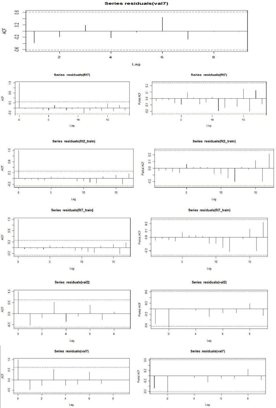
Figure 14 ACF and PACF plots for full model, training and testing for Production of Groundnut.

Results of the model are given in the Tables 3 and 4 for area and production, respectively. It was found that coefficients of the model ARIMA (2, 2, 2) are significant, and it clearly describes the behavior of the actual data series. The estimates AR (1) (Full model–1.024***, Training–1.067***), AR (2) (Full model–0.475***, Testing–0.419***) and MA (2) (Full model–0.639***, Training–0.643***) of the models were negatively significantly associated with area of groundnut, and the effect of MA (1) (Full model–0.179, Training–0.089) parameter wasn’t significant. The ARIMA model with parameters $p-2,d-1,q-1$ were found to be significant, both AR (1) and AR (2) had negative association and MA (1) had significant positive association. Both ARIMA (2,2,2) and ARIMA (2,1,1) were equally efficient in predicting the area of groundnut, while ARIMA (2,2,2) had less error estimates compared to ARIMA (2,1,1). These two models were better in case of model accuracy criteria’s among fitted models. The root mean square error value (RMSE) for ARIMA (2,2,2) was 0.43 when the model was fit to full data and training set, and during testing it was 0.47. The ARIMA (2,1,1) model produced RMSE value 0.44 during full model and training, and 0.51 in testing. These models also had the same trend in respect of other accuracy criteria’s such MAPE (ARIMA (2,2,2)-Full Model-5.1, Training-5.12 and Testing-6.43 & ARIMA(2,1,1)-Full Model-5.25, Training-5.37, Testing-7.28), ME, MAE, MPE, MASE and ACF (Table 5).

In case of model information criteria AIC and BIC, ARIMA with parameters $p-2,d-1,q-1$, showed minimum estimates of information criteria’s (AIC-85.83, BIC-94.47) while the ARIMA (2, 2, 2) model was slightly on the higher side (AIC-87.65, BIC-98.37), but it was better in terms of R-Square (0.84) when fitted to full data sets. Even during training and testing ARIMA (2, 1, 1) outperformed ARIMA (2, 2, 2) in terms of AIC and BIC (Table 5) while ARIMA (2, 2, 2) was better than other models in terms of R-Square value (Training-0.85, Testing-0.5) during full model, training and testing. Residuals of all the fitted models were normal as per box-pierce test while residuals of ARIMA (1,0,0) was significant for area when fitted to full data set (p-value-0.05) and was significant during training (p-value-0.034) for prediction of production of groundnut (Tables 5 and 7). Therefore, to predict the area of groundnut $p,d,q$ value in the range of 1–2 would be sufficient and these parameters were highly significant and exhibited better model accuracy criteria’s and residual characteristics. Plots of ACF and PACF confirms (ARIMA (2,1,1) and ARIMA (2,2,2)) (Figures 11 and 12) the adequacy of model for prediction purpose and actual v/s prediction plots of these two models exhibited similar trend (Figures 1–4) [19].

The same set of models were tried to fit the production data and it was found that these models were found better fitted. Both ARIMA (2,1,1) and ARIMA (2,2,2) fitted well to full data set and produced better estimates viz., RMSE and MAPE values (Table 7) than other models and while in training, ARIMA (2,2,2) was found to have better RMSE and MAPE value 1.050 and 12.955, respectively. During testing, these models fit well to the data set while the model with parameter $p-2,d-1,q-0$ was found better with low RMSE value 1.735. The models with parameter $p-2,d-1,q-1$ and $p-2,d-2,q-2$ were consistent in full model as well as in training, therefore, these models may be retained for future modeling of production of groundnut in India. The AIC and BIC values for ARIMA (1,1,1) for full and training were found better in comparison to other models, but coefficient of determination value for ARIMA (2, 2, 2) were better for full (54.2%) and training data (59.1%) sets while it predicted the test data with less R-Square (5.8%). Therefore, whenever the model is developed on full data set and utilizing it for forecasting purpose, models some time failed to forecast accurately in case of out sample forecast $(Y_{t+1})$, and while evaluating prediction accuracy model, stability is always an issue [4]. Therefore, parameter range for $p$ (Autoregressive) is 1–2, $d$ (Differencing) – 1–2 and for $q$ (Moving Average) – 1–2 would be sufficient for model building for production of groundnut in India. Plots of ACF were found adequate for full training data sets, while for testing sets, none of the models were significantly predicted and the residuals characteristics were non normal (Figures 13 and 14). Plots of actual and predicted values form above models for full, and training data sets were satisfactory while for testing sets none of the models satisfactorily predicted the actual (Figures 5 and 6). Furthermore, best model may also be chosen based on the accumulated prediction error [8].

Comparison of Feed-forward neural network and ARIMA

In capturing the complex nonlinearity in a data series, neural networks are more effective and preferred in place of ARIMA models. The model criteria’s obtained are average of 10 networks. The results from the Table 6 revealed that the full data is fitted using feed-forward 4-2-1 network, i.e., the network utilizes four lagged values ($t-1,t-2,t-3,t-4$. etc.) of time series as input, which is connected by two hidden nodes to hidden layer and connected to a single output layer. For predicting the area of groundnut (Full model), ANN predicted with RMSE value 0.372, MAPE 4.302 and with R-Square 0.839. In training and testing, ANN was found to be the best when fitted to data with minimum estimates of error (Training-RMSE – 0.369, MAPE – 4.116) [15] and model r-square (Training-81%, Testing-60.2%). On comparison, ARIMA models also produced better R-Square during full data (ARIMA (2,1,1) – 0.83 & ARIMA (2,2,2) – 0.843) and training sets while they failed to outperform ANN during testing [1]. Forecasting accuracy of feed-forward neural network models was consistent with respect to RMSE and MAPE and R-Square in all three stages of model fitting, i.e., complete, training and testing. Because a neural network model learns the data, captures the nonlinearity in the data series efficiently, and finally, predicts more accurately than the ARIMA models. Therefore, neural networks were better preferred in place of 2-ARIMA models for predicting area of groundnut [1].

The same trend was observed when these models were fit to production data of groundnut. A neural network model with 3 inputs, 2 hidden and 1 output units predicted the production data accurately as compared to ARIMA models. The model ARIMA (2, 2, 2) exhibited better accuracy criteria’s when fitted to full data set and training set but for testing set its accuracy declined drastically i.e., it predicted testing data series with low r-square (0.058). While ARIMA (2, 1, 1) was better compared to ARIMA (2, 2, 2) while fitted to testing data set with 26.6% r-square value. In terms of RMSE (Full-0.911, Training-0.852, Testing-1.055), MAPE (Full-11.729, Training-10.970, Testing-13.518) value NN outperformed ARIMA models (Table 8). Plots also confirmed that NN models predicted the direction of actual values accurately (Figures 7–10). Model with parameters $p-2,d-1-2,q-1-2$ produced better r-square and other accuracy criteria’s when fitted to all the data series except testing in predicting production [28].

Conclusion

For better planning of agriculture production these prediction models will be extremely helpful for the farming community. These real insights will be helpful for the policy makers to bring the significant changes in leading areas of production. Most importantly price volatility in the markets may be stabilized to a greater extent through marketing management by knowing the expected area and production of the crop. As per the above results feed-forward neural network converges at a faster rate to local minima and has capacity to analyze complex data structure [22]. Time series models are better predictive models when full data sets are used but the model accuracy declines when the data is split into training and testing. Since ANN models are mainly meant for complex nonlinear data sets and predict consistently when the data set is divided into training and testing sets. To choose appropriate p, d, q parameters auto.arima function of r-studio may be used and Box-Jenkin models perform better when the data is linear.

References

[1] Adebiyi, Ayodele Adewumi, Aderemi and Ayo Charles. (2014). Comparison of ARIMA and Artificial Neural Networks Models for Stock Price Prediction. Journal of Applied Mathematics. 1–7, 10.1155/2014/614342.

[2] Annonymous, Consortium of e-Resource Agriculture – DKMA, 2020.Indiastat.com

[3] Balanagammal, D., Ranganathan, C.R. and Sundaresan, K. (2000). Forecasting of agricultural scenario in Tamilnadu – A time series analysis. Journal of Indian Society of Agricultural Statistics. 53(3), 273–286.

[4] Biljana Petrevska. (2017). Predicting tourism demand by A.R.I.M.A. models, Economic Research. Ekonomska Istraživanja. 30(1), 939–950, DOI: 0.1080/1331677X.2017.1314822

[5] Box, G. E. P. and Jenkins, G. M. (1976) Time Series Analysis, Forecasting and Control. San Francisco, Holden- Day, California, USA.

[6] Chattopadhyay Surajit and Bandyopadhyay Goutami. (2007). Artificial neural network with backpropagation learning to predict mean monthly total ozone in Arosa, Switzerland. International Journal of Remote Sensing. INT J REMOTE SENS. 28, 4471–4482. 10.1080/01431160701250440.

[7] Darekar Ashwini and Reddy Amarender, A. (2017). Forecasting of Common Paddy Prices in India. Journal of Rice Research.:10. 71–75. 10.2139/ssrn.3064080.

[8] Eric Jan Wagenmakersa, Peter Grunwaldb, and Mark Steyvers. (2006). Accumulative prediction error and the selection of time series models. Journal of Mathematical Psychology. 50, 149–166

[9] Estrada Francisco, Gay Garcia Carlos and Conde Cecilia. (2012). A methodology for the risk assessment of climate variability and change under uncertainty. A case study: Coffee production in Veracruz, Mexico. Climatic Change. 113, 10.1007/s10584-011-0353-9.

[10] Fattah Jamal, Ezzine Latifa, Aman Zineb, Moussami Haj and Lachhab Abdeslam. (2018). Forecasting of demand using ARIMA model. International Journal of Engineering Business Management. 10. 184797901880867. 10.1177/1847979018808673.

[11] He Angela W.W., Kwok Jerry T.K., and Wan Alan T.K. (2010). An empirical model of daily highs and lows of West Texas Intermediate crude oil prices. Energy Economics, Elsevier. vol. 32(6), pages 1499–1506.

[12] Hemavathi, M. and Prabakaran, K. (2018). ARIMA Model for Forecasting of Area, Production and Productivity of Rice and Its Growth Status in Thanjavur District of Tamil Nadu, India. Int.J.Curr.Microbiol.App.Sci. 7(2), 149–156. doi: https://doi.org/10.20546/ijcmas.2018.702.019

[13] Juang W.C, Huang S.J, and Huang F.D. (2017). Application of time series analysis in modelling and forecasting emergency department visits in a medical centre in Southern Taiwan. BMJ Open, 7:e018628. doi:10.1136/ bmjopen-2017-018628.

[14] Kannan Govind, Gosukonda Ramana and Mahapatra Ajit. (2019). Prediction of Stress Responses in Goats: Comparison of Artificial Neural Network and Multiple Regression Models. Canadian Journal of Animal Science. 100, 10.1139/CJAS-2019-0028.

[15] Liu Qiao, Li Zhongqi, Ji Ye, Martinez Leonardo, Ul-Haq Zia, Javaid Arshad, lu Weiand Wang and Jianming. (2019). Forecasting the seasonality and trend of pulmonary tuberculosis in Jiangsu Province of China using advanced statistical time-series analyses. Infection and Drug Resistance. Volume 12, 2311–2322. 10.2147/IDR.S207809.

[16] Margaretha Ohyvera, and Herena Pudjihastutib. (2018). ARIMA Model for Forecasting the Price of Medium Quality Rice to Anticipate Price Fluctuations. Procedia Computer Science. 135, 707–711.

[17] Martin Haugh. (2016). Risk Management and Time Series. IEOR E4602: Quantitative Risk Management. 1–6.

[18] Merh Nitin, Saxena Vinod and Pardasani Kamal. (2010). A comparison between Hybrid Approaches of ANN and ARIMA for Indian Stock Trend Forecasting. Business Intelligence Journal. 3, 23–44.

[19] Mondal Prapanna, Shit Labani and Goswami Saptarsi. (2014). Study of Effectiveness of Time Series Modeling (ARIMA) in Forecasting Stock Prices. International Journal of Computer Science, Engineering and Applications. 4, 13–29. 10.5121/ijcsea.2014.4202.

[20] Paul Jiban, Hoque Md and Rahman Mohammad. (2013). Selection of Best ARIMA Model for Forecasting Average Daily Share Price Index of Pharmaceutical Companies in Bangladesh: A Case Study on Square Pharmaceutical Ltd. Global Journal of Management and Business Research. 13, 14–25.

[21] Pushpa M. Savadatti. (2017). Trend and forecasting analysis of area, production and productivity of total pulses in India. Indian Journal of Economics and Development. Vol 5 (12), December.

[22] Qiu M. and Song Y. (2016). Predicting the Direction of Stock Market Index Movement Using an Optimized Artificial Neural Network Model. PLoS ONE. 11(5), e0155133. doi:10.1371/journal. pone.0155133

[23] R Core Team. (2017). R A language and environment for statistical computing. R Foundation for Statistical Computing, Vienna, Austria. URL https://www.R-project.org/.2017.

[24] Rundo Francesco, Trenta Francesca, Stallo Agatino and Battiato Sebastiano. (2019). Machine Learning for Quantitative Finance Applications: A Survey. Applied Sciences. 9, 1–20. 10.3390/app9245574.

[25] Sharma Pawan. (2018). Forecasting Maize Production in India using ARIMA Model. 10, 30954/2394-8159.01.2018.1.

[26] Siami Namini, Sima Tavakoli, Neda Siami and Namin Akbar. (2018). A Comparison of ARIMA and LSTM in Forecasting Time Series. 1394–1401. 10.1109/ICMLA.2018.00227.

[27] Tripathi Rahul, Nayak A. K, Raja R. Shahid, Mohammad Kumar, Anjani Mohanty, Sangita Panda, Bipin Lal, B. and Gautam Priyanka. (2014). Forecasting Rice Productivity and Production of Odisha, India, Using Autoregressive Integrated Moving Average Models. Advances in Agriculture. 10, 1155/2014/621313.

[28] Vijay Shankar Pandey, and Abhishek Bajpai. (2019). Predictive Efficiency of ARIMA and ANN Models: A Case Analysis of Nifty Fifty in Indian Stock Market. International Journal of Applied Engineering Research. ISSN 0973-4562. Volume 14(2), 232–244.

Biographies

S. T. Pavan Kumar is an Assistant Professor (Statistics) at College of Community Science, Central Agricultural University (Imphal), Tura, Meghalaya. He attended the Bidhan Chandra Krishi Viswavisyalaya, West Bengal, from where he received Ph.D (Agricultural Statitsics) in the year 2017. He published 12 research articles and chapters in the field of statistics in the national, international journals and training manuals.

Ferdinand B. Lyngdoh is an Assistant Professor (English) at College of Community Science, Central Agricultural University (Imphal), Tura, Meghalaya. He is currently pursuing his doctoral degree from the North Eastern Hill University (NEHU), Tura Campus.

Journal of Reliability and Statistical Studies, Vol. 13_2-4, 265–286.
doi: 10.13052/jrss0974-8024.13244
© 2020 River Publishers

Abstract

Introduction

Methodology

Data for the Study

Workflow and Methods: Identification and Estimation

Results and Discussion

Comparison of Feed-forward neural network and ARIMA

Conclusion

References

Biographies