Bayesian Estimation of Transmuted Weibull Distribution under Different Loss Functions

Rahila Yousaf¹, Sajid Ali^2,* and Muhammad Aslam¹

¹Department of Mathematics and Statistics, Riphah International University, Islamabad 46000, Pakistan

²Department of Statistics, Quaid-i-Azam University, Islamabad 45320, Pakistan

E-mail: ejazraheela@yahoo.com; sajidali.qau@hotmail.com; m.aslam@riphah.edu.pk

*Corresponding Author

Received 22 July 2020; Accepted 01 November 2020; Publication 29 December 2020

Abstract

In this article, we aim to estimate the parameters of the transmuted Weibull distribution (TWD) using Bayesian approach, as the Weibull distribution plays an important role in reliability engineering and life testing problems. Informative and non-informative priors under squared error loss function (SELF), precautionary loss function (PLF) and quadratic loss function (QLF) are assumed to estimate the scale, the shape and the transmuted parameter of the TWD. In addition to this, we also compute the Bayesian credible intervals (BCIs). To estimate parameters, we adopt Markov Chain Monte Carlo (MCMC) technique assuming uncensored and censored environments in terms of different sample sizes and censoring rates. The posterior risks, associated with each estimator are used to compare the performance of different estimators. Two real data sets are analyzed to illustrate the flexibility of the proposed distribution.

Keywords: Transmuted Weibull distribution, loss functions, Bayes estimators, posterior risks, uniform prior, informative prior, BCIs, MCMC, censoring and chi-square test.

1 Introduction and Motivation

Statistical distributions are very useful in describing and predicting real world phenomena. However, due to recent developments in data gathering mechanism the available probability models do not properly fit data in many important and practical problems. In such cases, non-parametric models may be recommended, but the popularity of parametric models is undeniable. Shaw and Buckley (2009) used the quadratic rank transmutation map (QRTM) technique to construct new families of non-Gaussian distributions. In fact, this technique is used to modify the moments, skewness and kurtosis of a baseline distribution (Al- Kadim and Mohammed, 2017). The resulted distribution is known as the transmuted distribution. This family gained attention of many researchers and as a result, many new flexible distributions have been developed and studied over the past decade. For example, Khan and King (2013) introduced the transmuted modified Weibull distribution while Ebraheim (2014) introduced exponentiated transmuted Weibull distribution. Recently, Al- Kadim and Mohammed (2017) constructed a new lifetime distribution, known as the transmuted cubic Weibull distribution. Mobarak et al., (2017) introduced a new weighted distribution called the size biased weighted transmuted Weibull distribution. Abdurrahman (2017) used the method of least squares and method of moments to estimate parameters of transmuted Weibull distribution and compared them through a simulation study under statistical measure like mean squared error (MSE). Ahmad et al. (2015) discussed some structural properties of transmuted Weibull distribution, including mean, harmonic mean, standard deviation, moment generating function (MGF), skewness and kurtosis. Currently, transmuted distributions are applied in many areas such as reliability studies, lifetime analysis, engineering, economics, insurance and environmental sciences (Shaw and Buckley, 2009).

A random variable $X$ is said to have transmuted probability distribution if its probability density function (pdf) and cumulative distribution function (CDF) can be written as (Shaw and Buckley, 2009):

$f(x)=g(x)[1+\lambda -2\lambda G(x)]$	(1)
$F(x)=(1+\lambda )G(x)-\lambda G^2(x)$	(2)

where $x>0$ and $|\lambda |\le 1$ is the transmuted parameter, $G(x)$ denotes the CDF of the baseline distribution, $f(x)$ and $F(x)$ are the associated transmuted pdf and CDF, respectively.

The Weibull distribution is a very popular lifetime probability distribution and used in many different areas of reliability and survival analysis. Much of the attractiveness of the Weibull distribution is due to the wide variety of shapes which can be generated by altering its shape parameter. Moreover, it is a versatile distribution because many other distributions, like exponential, Rayleigh, are special cases of this flexible distribution. Despite its popularity, and wide applicability, the traditional Weibull distribution is unable to capture the entire lifetime phenomenon. For instance, the Weibull distribution is not suitable for the data set which has a non-monotonic failure rate. Therefore, some generalizations of the Weibull distribution have been studied. For example, a generalization of the Weibull distribution with application to the analysis of survival data is given by Mudholkar, Srivastava, and Kollia (1996). Khan and King (2014) proposed transmuted generalize inverse Weibull distribution and discussed some of its mathematical properties. The authors also used the method of maximum likelihood to estimates the parameters. Khan et al. (2016) introduced transmuted generalized Weibull distribution and explored its mathematical properties including expressions for the quantile function, moments, entropies, mean deviation, Bonferroni and Lorenz curves and moments of the order statistics. The authors also used the method of maximum likelihood to estimate model parameters. Similarly Nofal et al. (2017) proposed the generalized transmuted Weibull distribution and derived its properties.

In this article, we focus on the Bayesian analysis of the transmuted Weibull distribution introduced by Aryal and Tsokos (2011), which is a generalization of the Weibull probability distribution. We particularly focus on the Bayesian analysis because Abdurrahman (2017) used the method of maximum likelihood and the method of moment estimators to estimate the parameters of the transmuted Weibull distribution. To this end, we devise a Markov Chain Monte Carlo algorithm to compute the posterior summaries of the unknown parameters of the said distribution. We compare results by assuming different priors, loss functions, and various choices of sample size and different sets of parameters.

The rest of the paper is organized as follows: Section 2 defines the transmuted Weibull distribution, its likelihood function, expressions for the posterior distributions using non-informative and informative priors and marginal posterior densities for censored and uncensored data, respectively. Expressions of the Bayes estimators (BEs) and their respective posterior risks (PRS) under different loss functions are discussed in Section 3. Estimation of the unknown parameters of the proposed distribution by MCMC algorithm to compute the posterior summaries is also given in the same section. A simulation study under different loss functions and different types of priors is presented in Section 4. In Section 5, the Bayesian credible intervals (BCI) are discussed mathematically and numerically. Two real-life data sets have been analyzed in Section 6 while Section 7 concludes the article.

2 Transmuted Weibull Distribution

A random variable ‘X’ follows a Weibull distribution with parameters $\alpha >0$ and $\beta >0$, if its probability density function is of the form:

$$g(x;\alpha ,\beta )=\frac{\alpha }{\beta }{x}^{\alpha -1}\exp \left(-\frac{x^{\alpha }}{\beta }\right),x\ge 0$$

The cumulative distribution function (CDF) of the Weibull distribution is:

$$G(x)=1-\exp \left(-\frac{{\mathrm{x}}^{\alpha }}{\beta }\right)$$

(3)

where $\alpha$ denotes the shape parameter and $\beta$ is the scale parameter. To obtain the CDF of transmuted Weibull distribution, we substitute the value of G(x) in Equation (2), which is

$$F(x)=(1+\lambda )\left\{1-\exp \left(-\frac{{\mathrm{x}}^{\alpha }}{\beta }\right)\right\}-\lambda {\left\{1-\exp \left(-\frac{{\mathrm{x}}^{\alpha }}{\beta }\right)\right\}}^2$$

After some algebraic simplifications, we get

$$F(x;\alpha ,\beta ,\lambda )=\exp \left(-\frac{{\mathrm{x}}^{\alpha }}{\beta }\right)\left\{1-\lambda +\lambda \exp \left(-\frac{{\mathrm{x}}^{\alpha }}{\beta }\right)\right\}$$

(4)

which is the required CDF of the transmuted Weibull distribution. Now, to find the PDF of the transmuted Weibull distribution, we differentiate Equation (4) with respect to ‘x’ and simplify it. The resulting PDF is

$f(x;\alpha ,\beta ,\lambda )$	$={\displaystyle \frac{\alpha }{\beta }}{x}^{\alpha -1}\exp \left(-{\displaystyle \frac{{\mathrm{x}}^{\alpha }}{\beta }}\right)\left\{1-\lambda +2\lambda \exp \left(-{\displaystyle \frac{{\mathrm{x}}^{\alpha }}{\beta }}\right)\right\},$
$x$	$\ge 0,\alpha ,\beta >0\mathrm{and}|\lambda |\le 1$	(5)

Special Cases

• If $\lambda =0$, then Transmuted Weibull distribution reduces to the ordinary Weibull distribution.

• If $\alpha =1$ then we obtained transmuted exponential distribution. In addition, if $\lambda =0$, we get the ordinary exponential distribution.

• If $\alpha =\beta =1$ then the resulting distribution is known as transmuted standard exponential distribution.

• If $\alpha =2$ then we have transmuted Rayleigh distribution. Also, if $\lambda =0$, we get the traditional Rayleigh distribution.

Next, we discuss the likelihood function for Equation (2).

2.1 Likelihood Functions for Different Sampling Schemes

Let $X{}_1$, $X{}_2,\mathrm{\dots },X_n$ be a complete random sample of size n is taken from the transmuted Weibull distribution. Then, the likelihood function for the complete data set is:

$L(x;\alpha ,\beta ,\lambda )$	$={\left({\displaystyle \frac{\alpha }{\beta }}\right)}^n\exp \left\{-{\displaystyle \sum _{i=1}^n}{\displaystyle \frac{x_i^{\alpha }}{\beta }}\right\}{\displaystyle \prod _{i=1}^n}$
	$\mathrm{\hspace{1em}}\times \left[x_i^{\alpha -1}\left\{1-\lambda +2\lambda \exp \left(-{\displaystyle \frac{{\mathrm{x}}^{\alpha }}{\beta }}\right)\right\}\right]$
$L(x;\Omega )$	$={\left({\displaystyle \frac{\alpha }{\beta }}\right)}^n\mathrm{𝑒𝑥𝑝}\left\{-{\displaystyle \sum _{i=1}^n}{\displaystyle \frac{x_i^{\alpha }}{\beta }}\right\}\mathrm{𝑒𝑥𝑝}\left\{\left(\alpha -1\right){\displaystyle \sum _{i=1}^n}{\mathrm{𝑙𝑜𝑔𝑥}}_i\right\}\mathrm{𝑒𝑥𝑝}$
	$\mathrm{\hspace{1em}}\times \left[{\displaystyle \sum _{i=1}^n}\mathrm{𝑙𝑜𝑔}\left\{1-\lambda +\mathit{2}\lambda \mathrm{𝑒𝑥𝑝}\left(-{\displaystyle \frac{x_i^{\alpha }}{\beta }}\right)\right\}\right]$

where $\mathrm{\Omega }=(\alpha ,\beta ,\lambda )$ and $x={𝒙}_1,{𝒙}_2,\mathrm{\dots },{𝒙}_n$. After simplification, we get

$L(x;\mathrm{\Omega })$	$={\alpha }^n\mathrm{𝑒𝑥𝑝}\left\{(\alpha -1){\displaystyle \sum _{i=1}^n}{\mathrm{𝑙𝑜𝑔𝑥}}_i\right\}{\displaystyle \frac{1}{{\beta }^n}}\mathrm{𝑒𝑥𝑝}\left(-{\displaystyle \frac{{\sum }_{i=1}^n{x}_i^{\alpha }}{\beta }}\right)\mathrm{𝑒𝑥𝑝}$
	$\mathrm{\hspace{1em}}\times \left[{\displaystyle \sum _{i=1}^n}\mathrm{𝑙𝑜𝑔}\left\{1-\lambda +\mathit{2}\lambda \mathrm{𝑒𝑥𝑝}\left(-{\displaystyle \frac{x_i^{\alpha }}{\beta }}\right)\right\}\right]$	(6)

In many life testing experiments, we cannot collect complete data on failure times due to time and cost restrictions. Thus, censoring is an important aspect of the lifetime data (Romeu, 2004; Gijbels, 2010; and Kalbfleisch and Prentice, 2011). Suppose $𝐗=(X_1,X_2,X_3,\mathrm{\dots },X_r)$ is a type-I censored sample of size r from n items whose lifetimes belong to transmuted Weibull distribution with parameters $\alpha ,\beta$ and $\lambda$. It is worth mentioning that in type-I censoring, the censoring time is fixed in advanced whereas number of failures are random. We put n items on the life test and observe that r failures $t_1,t_2,\mathrm{\dots },t_r$, where r is an integer number lies between 0 to n and $(n-r)$ denotes the number of survived/uncensored items. According to Mendenhall and Hader (1958), the likelihood function for censored data is:

$$L(x;\mathrm{\Omega })\propto \left[\prod _{j=1}^{r}f(x_j)\right]{[1-F(T)]}^{n-r}$$

where $T$ denotes time, r denotes the number of censored observations and (n-r) are uncensored observations. The simplified form of the likelihood function assuming transmuted Weibull distribution for censored data is

$L(x;\mathrm{\Theta })$	$\propto {\alpha }^r\exp \left(-\alpha {\displaystyle \sum _{j=1}^r}\log {\displaystyle \frac{1}{x_j}}\right){\displaystyle \frac{1}{{\beta }^r}}\exp \left(-{\displaystyle \frac{{\sum }_{j=1}^r{x}_j^{\alpha }}{\beta }}\right)$
	$\mathrm{\hspace{1em}}\times \exp \left[{\displaystyle \sum _{j=1}^r}\log \left\{1-\lambda +2\lambda \exp \left(-{\displaystyle \frac{x_j^{\alpha }}{\beta }}\right)\right\}\right]$
	$\mathrm{\hspace{1em}}\exp ((n-r)\log [1-\exp (-{\displaystyle \frac{T^{\alpha }}{\beta }})$
	$\times \{1-\lambda +\lambda \exp (-{\displaystyle \frac{T^{\alpha }}{\beta }})\}])$

Next, we discuss the posterior distribution, which is obtained by the celebrated Bayes theorem, $g(\alpha |𝐱)=\frac{𝐋(𝐱;𝜶)𝝅(𝜶)}{{\int }_{\alpha }^{\mathrm{\infty }}𝐋(𝐱;𝜶)𝝅(𝜶)𝐝𝜶}$, where $𝝅(𝜶)$ denotes the joint prior distribution of $𝜶=({\alpha }_1,{\alpha }_2,\mathrm{\dots }{\alpha }_k)$, $𝐋(𝐱;𝜶)$ denote the likelihood function and $𝒈(𝜶|𝐱)$ is the joint posterior distribution.

2.2 Posterior Distribution using Uniform Prior (UP)

To estimate the unknown parameters in Bayesian, we need to specify a prior for each parameter that should not be directly specified by a model itself (Lawrence et al., 2013). Contrary to the frequentist approach, Bayesian approach utilizes the prior knowledge about the parameters as well as the observed data. If prior knowledge about the parameters is not available, it is possible to make use of the non-informative prior in Bayesian analysis. In short, non-informative prior is a prior which expresses vague information about the parameters.

To estimate the unknown parameters of the transmuted Weibull distribution, we have assumed $\alpha \propto 1,\forall \alpha \in (0,\mathrm{\infty })$, $\beta \propto 1,\forall \beta \in (0,\mathrm{\infty })$ and $\lambda \propto 1,\forall \lambda \in (-1,1)$. Assuming independence among parameters, the joint prior distribution of parameters $\alpha$, $\beta$ and $\lambda$ is:

$${\pi }_1(\alpha ,\beta ,\lambda )\propto 1\mathit{\hspace{1em}}\alpha ,\beta >0\mathit{\hspace{1em}}\mathrm{and}\mathit{\hspace{1em}}|\lambda |\le 1$$

Using the Bayes theorem $g(\alpha ,\beta ,\lambda |𝐱)=\frac{L(x;\alpha ,\beta ,\lambda )\pi (\alpha ,\beta ,\lambda )}{{\int }_0^{\mathrm{\infty }}{\int }_0^{\mathrm{\infty }}{\int }_{-1}^{1}L(x;\alpha ,\beta ,\lambda )\pi (\alpha ,\beta ,\lambda )𝑑\lambda 𝑑\beta 𝑑\alpha }$, the joint posterior distribution of parameters $\alpha$, $\beta$ and $\lambda$ given data $𝐱$ assuming uniform prior is:

$g(\alpha ,\beta ,\lambda |x)$	$={\displaystyle \frac{\begin{array}{c}{\alpha }^n\mathrm{𝑒𝑥𝑝}\left(-\alpha {\sum }_{i=1}^n\mathrm{𝑙𝑜𝑔}\frac{1}{x_i}\right)\frac{1}{{\beta }^n}\mathrm{𝑒𝑥𝑝}\left(-\frac{{\sum }_{i=1}^n{x}_i^{\alpha }}{\beta }\right)\hfill \\ \mathrm{𝑒𝑥𝑝}\left[{\sum }_{i=1}^n\mathrm{𝑙𝑜𝑔}\left\{1-\lambda +\mathit{2}\lambda \mathrm{𝑒𝑥𝑝}\left(-\frac{x_i^{\alpha }}{\beta }\right)\right\}\right]\hfill \end{array}}{\begin{array}{c}{\int }_0^{\mathrm{\infty }}{\int }_0^{\mathrm{\infty }}{\int }_{-1}^1{\alpha }^n\mathrm{𝑒𝑥𝑝}\left(-\alpha {\sum }_{i=1}^n\mathrm{𝑙𝑜𝑔}\frac{1}{x_i}\right)\frac{1}{{\beta }^n}\mathrm{𝑒𝑥𝑝}\left(-\frac{{\sum }_{i=1}^n{x}_i^{\alpha }}{\beta }\right)\hfill \\ \mathrm{𝑒𝑥𝑝}\left[{\sum }_{i=1}^n\mathrm{𝑙𝑜𝑔}\left\{1-\lambda +2\lambda exp\left(-\frac{x_i^{\alpha }}{\beta }\right)\right\}\right]d\lambda d\beta d\alpha \hfill \end{array}}}$
$g(\alpha ,\beta ,\lambda |x)$	$={\displaystyle \frac{{\alpha }^{A_{\mathit{01}}-1}\mathrm{𝑒𝑥𝑝}(-\alpha A_{\mathit{11}})\frac{1}{{\beta }^n}\mathrm{𝑒𝑥𝑝}\left(-\frac{A_{\mathit{21}}}{\beta }\right)\mathrm{𝑒𝑥𝑝}(A_{\mathit{31}})}{\begin{array}{c}{\int }_0^{\mathrm{\infty }}{\int }_0^{\mathrm{\infty }}{\int }_{-1}^1{\alpha }^{A_{\mathit{01}}-1}\mathrm{𝑒𝑥𝑝}(-\alpha A_{\mathit{11}})\frac{1}{{\beta }^n}\hfill \\ \mathrm{𝑒𝑥𝑝}\left(-\frac{A_{\mathit{21}}}{\beta }\right)\mathrm{𝑒𝑥𝑝}(A_{\mathit{31}})d\lambda d\beta d\alpha \hfill \end{array}}}$	(7)

where $A_{01}=n+1,$ $A_{11}={\sum }_{i=1}^n\log \frac{1}{x_i}$, $A_{21}={\sum }_{i=1}^n{x}_i^{\alpha }$ and $A_{31}={\sum }_{i=1}^n\log \left\{1-\lambda +2\lambda \exp \left(-\frac{x_i^{\alpha }}{\beta }\right)\right\}$

Similarly, for censored data, the posterior distribution is:

$$g(\alpha ,\beta ,\lambda |x)=\frac{{\alpha }^{B_{\mathit{01}}-1}\mathrm{𝑒𝑥𝑝}(-\alpha B_{\mathit{11}})\frac{1}{{\beta }^r}\mathrm{𝑒𝑥𝑝}\left(-\frac{B_{\mathit{21}}}{\beta }\right)\mathrm{𝑒𝑥𝑝}(B_{\mathit{31}})}{\begin{array}{c}{\int }_0^{\mathrm{\infty }}{\int }_0^{\mathrm{\infty }}{\int }_{-1}^1{\alpha }^{B_{\mathit{01}}-1}\mathrm{𝑒𝑥𝑝}(-\alpha B_{\mathit{11}})\frac{1}{{\beta }^r}\hfill \\ \mathrm{𝑒𝑥𝑝}\left(-\frac{B_{\mathit{21}}}{\beta }\right)\mathrm{𝑒𝑥𝑝}(B_{\mathit{31}})d\lambda d\beta d\alpha \hfill \end{array}}$$

(8)

where

$$B_{\mathit{01}}=r+1,B_{\mathit{11}}=\sum _{j=1}^r\mathrm{𝑙𝑜𝑔}\frac{1}{x_j},B_{\mathit{21}}=\sum _{j=1}^r{x}_j^{\alpha }$$

and

$B_{31}$	$={\displaystyle \sum _{j=1}^r}\log \left\{1-\lambda +2\lambda \exp \left(-{\displaystyle \frac{x_j^{\alpha }}{\beta }}\right)\right\}+\left(n-r\right)\log$
	$\mathrm{\hspace{1em}}\times \left[1-\exp \left(-{\displaystyle \frac{T^{\alpha }}{\beta }}\right)\left\{1-\lambda +\lambda \exp \left(-{\displaystyle \frac{T^{\alpha }}{\beta }}\right)\right\}\right].$

As the posterior distributions are not in closed form for both the censored and the uncensored data, the marginal posterior densities of parameters $\alpha$, $\beta$ and $\lambda$ for uncensored and censored data are obtained by integrating out the nuisance parameters, i.e., $g(\alpha |𝐱)={\int }_{\beta }{\int }_{\lambda }g(\alpha ,\beta ,\lambda |x)𝑑\beta 𝑑\lambda$ and vice versa. Thus, we use the MCMC technique to obtain the posterior summaries.

Next, we discuss the derivation of the posterior distribution assuming informative prior.

2.3 Posterior Distribution using Informative Prior (IP)

An an informative prior provides specific and definite information about parameters in the form of probability distribution (Aslam et al., 2014). In our study, we assumed that the prior distributions of $\alpha$, $\beta$ and $\lambda$ are independent (Punt and Walker, 1998; Punt and Butterworth, 2000). To be more specific, we assume $\alpha \sim gamma(a,b)$, $\beta \sim \mathrm{inverse}\mathrm{gamma}(c,d)$ and $\lambda \sim \mathrm{uniform}(l_1,l_2)$. The joint prior of parameters $\alpha$, $\beta$ and $\lambda$ is:

$$g(\alpha ,\beta ,\lambda )\propto {\alpha }^{a-1}{e}^{-b\alpha }\frac{1}{{\beta }^{c+1}}{e}^{-\frac{d}{\beta }}\frac{1}{l_2-l_1}$$

The joint posterior distribution of parameters $\alpha$, $\beta$ and $\lambda$ given data $x$ assuming IP for complete data is:

$g(\alpha ,\beta ,\lambda |𝐱)$	$={\displaystyle \frac{\begin{array}{c}{\alpha }^{n+a-1}\exp \left\{-\alpha \left(b+\sum \log \frac{1}{x_i}\right)\right\}\frac{1}{{\beta }^{n+c+1}}\hfill \\ \exp \left\{-\frac{1}{\beta }\left(d+\sum x_i^{\alpha }\right)\right\}\hfill \\ \exp \left[\sum \log \left\{1+\lambda -2\lambda \exp \left(-\frac{x_i^{\alpha }}{\beta }\right)\right\}\right]\hfill \end{array}}{\begin{array}{c}{\int }_0^{\mathrm{\infty }}{\int }_0^{\mathrm{\infty }}{\int }_{-1}^1{\alpha }^{n+a-1}\hfill \\ \exp \left\{-\alpha \left(b+\sum \log \frac{1}{x_i}\right)\right\}\frac{1}{{\beta }^{n+c+1}}\hfill \\ \exp \left\{-\frac{1}{\beta }\left(d+\sum x_i^{\alpha }\right)\right\}\hfill \\ \exp \left[\sum \log \left\{1+\lambda -2\lambda \exp \left(-\frac{x_i^{\alpha }}{\beta }\right)\right\}\right]d\lambda d\alpha d\beta \hfill \end{array}}}$	(9)
$g(\alpha ,\beta ,\lambda |𝐱)$	$={\displaystyle \frac{\begin{array}{c}{\alpha }^{C_{11}-1}\exp \left(-\alpha D_{11}\right)\frac{1}{{\beta }^{C_{21}-1}}\hfill \\ \exp \left(-\frac{D_{21}}{\beta }\right)\exp \left(D_{31}\right)\hfill \end{array}}{\begin{array}{c}{\int }_0^{\mathrm{\infty }}{\int }_0^{\mathrm{\infty }}{\int }_{-1}^1{\alpha }^{C_{11}-1}\hfill \\ \exp \left(-\alpha D_{11}\right)\frac{1}{{\beta }^{C_{21}-1}}\hfill \\ \exp \left(-\frac{D_{21}}{\beta }\right)\exp \left(D_{31}\right)d\lambda d\alpha d\beta \hfill \end{array}}}\mathit{\hspace{1em}}\alpha ,\beta >0,|\lambda |\le 1$	(10)

where

$$C_{\mathit{11}}=n+a,D_{\mathit{11}}=b+\mathrm{𝑙𝑜𝑔}\frac{1}{x_i},C_{\mathit{21}}=n+c,D_{\mathit{21}}=d+\sum x_i^{\alpha }$$

and

$$D_{31}=\sum \log \left\{1-\lambda +2\lambda \exp \left(-\frac{x_i^{\alpha }}{\beta }\right)\right\}$$

For censored data, the joint posterior distribution of $\alpha$, $\beta$ and $\lambda$ given data is:

$g(\alpha ,\beta ,\lambda |x)={\displaystyle \frac{\begin{array}{c}{\alpha }^{C_{11}-1}\exp \left(-\alpha D_{12}\right)\frac{1}{{\beta }^{C_{21}-1}}\hfill \\ \exp \left(-\frac{D_{22}}{\beta }\right)\exp \left(D_{32}\right)\hfill \end{array}}{\begin{array}{c}{\int }_0^{\mathrm{\infty }}{\int }_0^{\mathrm{\infty }}{\int }_{-1}^1{\alpha }^{C_{11}-1}\hfill \\ \exp \left(-\alpha D_{12}\right)\frac{1}{{\beta }^{C_{21}-1}}\hfill \\ \exp \left(-\frac{D_{22}}{\beta }\right)\exp \left(D_{32}\right)d\lambda d\alpha d\beta \hfill \end{array}}}\mathit{\hspace{1em}}\alpha ,\beta >0,|\lambda |\le 1$

(11)

Where

$$C_{\mathit{12}}=r+a,D_{\mathit{12}}=b+\sum \mathrm{𝑙𝑜𝑔}\frac{1}{x_j},C_{\mathit{22}}=r+c,D_{\mathit{22}}=d+\sum x_j^{\alpha }$$

and

$D_{32}$	$={\displaystyle \sum _{j=1}^r}\log \left\{1-\lambda +2\lambda \exp \left(-{\displaystyle \frac{x_j^{\alpha }}{\beta }}\right)\right\}+\left(n-r\right)\log$
	$\mathrm{\hspace{1em}}\times \left[1-\exp \left(-{\displaystyle \frac{T^{\alpha }}{\beta }}\right)\left\{1-\lambda +\lambda \exp \left(-{\displaystyle \frac{T^{\alpha }}{\beta }}\right)\right\}\right].$

The marginal posterior densities of parameters $\alpha$, $\beta$ and $\lambda$ for uncensored and censored data are obtained by integrating out the nuisance parameters, i.e., $g(\alpha |𝐱)={\int }_{\beta }{\int }_{\lambda }g(\alpha ,\beta ,\lambda |x)𝑑\beta 𝑑\lambda$ and vice versa.

In the next section, we derive the Bayes estimators under different loss functions.

3 Bayes Estimators (BEs) and Posterior Risks (PRs) Under Different Loss Functions

To estimate the unknown parameter in Bayesian, we need to specify a loss function. The choice of a loss function depends on the considered problem; however, there are no rules how to select an appropriate loss function. There are two types of loss functions; symmetric and asymmetric. A loss function is called symmetric if it gives an equal weightage to over and under estimation otherwise non-symmetric. A loss function $L(\beta ,d)\ge 0$ represents a loss incurred when we estimate the unknown parameters $\alpha$, $\beta$ and $\lambda$ by $\widehat{\alpha }$, $\widehat{\beta }$ and $\widehat{\lambda }$ respectively for making a decision $d$. The worth of a decision is measured by the expected loss, which is known as the posterior risk. If $\widehat{d}$ is a Bayes estimator, then $\rho (\widehat{d})$ is called the posterior risk (Ali et al., 2012).

$$\rho (\widehat{d})=E_{\theta |x}\{L(\beta ,\widehat{d})\}=\int L(\beta ,\widehat{d})p(\beta |x)𝑑\beta$$

(12)

In this section, the Bayes estimators (BEs) and their respective posterior risk (PR) are computed under squared error loss function (SELF), precautionary loss function (PLF) and quadratic loss function (QLF). The square error loss function is a symmetric loss function which assigns equal losses to overestimation and underestimation. Norstrom (1996) discussed an alternative asymmetric precautionary loss function (PLF). The third loss function is QLF, which is another asymmetric loss function which approaches to infinity near the origin to avoid underestimation, and produces conservative estimators especially when underestimation may lead to serious consequence (Ali et al., 2013). The expressions of Bayes estimators under different loss functions with their respective posterior risk are given in Table 1.

Table 1 Bayes estimators and posterior risks of different loss functions

Loss Function	Expression	Bayes Estimators	Posterior Risks
SELF	$L(\beta ,d)={(\beta -d)}^{\mathit{2}}$	$\widehat{\mathrm{d}}={\mathrm{E}}_{\beta |\mathrm{x}}(\beta )$	$\rho (\widehat{\mathrm{d}})=\mathrm{E}({\beta }^2|𝐱)-{\{𝐄(\beta |𝐱)\}}^2$
PLF	$L(\beta ,d)=\frac{{(\beta -d)}^{\mathit{2}}}{d}$	$\widehat{\mathrm{d}}={\{\mathrm{E}({\beta }^2|𝐱)\}}^{\frac{1}{2}}$	$\rho (\widehat{\mathrm{d}})=2\{\mathrm{E}{({\beta }^2|𝐱\}}^{\frac{1}{2}}-2E(\beta |𝐱)$
QLF	$L(\beta ,d)={\left(\frac{\beta -d}{\beta }\right)}^{\mathit{2}}$	$\widehat{\mathrm{d}}=\frac{\mathrm{E}({\beta }^{-1}|𝐱)}{𝐄({\beta }^{-\mathrm{𝟐}}|𝐱)}$	$\rho (\widehat{\mathrm{d}})=1-\frac{{\{\mathrm{E}({\beta }^{-1}|𝐱)\}}^2}{𝐄({\beta }^{-2}|𝐱)}$

We refer to Ali (2015) for the derivation of Bayes estimators and posterior risks under these loss functions.

3.1 Posterior Summaries by Markov Chain Monte Carlo (MCMC)

From Equation (2.2), we observe that the expression of the posterior density is intractable form, and one needs a technique to solve it numerically for finding different posterior summaries. Thus, we adopt a Markov Chain Monte Carlo (MCMC) technique as have been used by Ali (2015) and Yousaf et al. (2018). To apply MCMC, the posterior densities assuming uniform and informative priors can be written as:

$g_{UP}(\alpha ,\beta ,\lambda |x)$

$\mathrm{\hspace{1em}\hspace{1em}}\propto f_{\alpha }(n+1,{\displaystyle \sum _{i=1}^n}\log {\displaystyle \frac{1}{x_i}})f_{\beta |\alpha }(n+1,{\displaystyle \sum _{i=1}^n}{x}_i^{\alpha })$

$\mathrm{\hspace{1em}\hspace{1em}}\mathit{\hspace{1em}\hspace{1em}}{f}_{\lambda }\left(\exp \left({\displaystyle \sum _{i=1}^n}\log \left\{1-\lambda +2\lambda \exp \left({\displaystyle \frac{x_i^{\alpha }}{\beta }}\right)\right\}\right)\right)$

$g_{IP}(\alpha ,\beta ,\lambda |x)$

$\mathrm{\hspace{1em}\hspace{1em}}\propto f_{\alpha }(a+n,{\displaystyle \sum _{i=1}^n}\log {\displaystyle \frac{1}{x_i}})f_{\beta |\alpha }(b+n,{\displaystyle \sum _{i=1}^n}{x}_i^{\alpha })$

$\mathrm{\hspace{1em}\hspace{1em}}\mathit{\hspace{1em}\hspace{1em}}{f}_{\lambda }\left(e+\exp \left({\displaystyle \sum _{i=1}^n}\log \left\{1-\lambda +2\lambda \exp \left({\displaystyle \frac{x_i^{\alpha }}{\beta }}\right)\right\}\right)\right)$

where $f_{\alpha }$ and $f_{\beta |\alpha }$ denote the probability density functions of the gamma and the inverse gamma distributions while $f_{\lambda }$ is the probability density functions of transmuted parameter. To obtain the Bayes estimates, their respective posterior risks and the associated Bayesian Credible intervals (BCI), we proceed as follows: Firstly, we generate a random sample from transmuted Weibull distribution, by using inverse integral transformation, i.e. $u_i=(1-e^{-\frac{x_i{}^{\alpha }}{\beta }})(1-\lambda +\lambda e^{-\frac{x_i{}^{\alpha }}{\beta }})$. After simplification we obtain

$$x_i={\left[-\beta \ln \left\{1-\left(\frac{1+\lambda -\sqrt{{(1+\lambda )}^2-4\lambda u_i}}{2\lambda }\right)\right\}\right]}^{\frac{1}{\alpha }}.$$

where $u{}_i\sim U(0,1)$ and $i=1,2,\mathrm{\dots },n.$ Thus, by providing the parameters’ values, one can obtain the desired random sample. To generate the censored data, one needs to fix time T and record units that are less than equal to censoring time. The number of units that are greater than censoring time would be considered censored observations.

Next, to implement the MCMC for obtaining the posterior summaries, we repeat the following steps of Gibbs sampling with Metropolis-Hasting step:

Algorithm 1.

1. Generate$\alpha \sim f_{\alpha }$, $\beta \sim f_{\beta |\alpha }$ and $\lambda \sim f_{\lambda }$.

2. Let $Y$ is called candidate distributions. Take $Y\sim Uniform(0,1)$.

3. Generate $U\sim Uniform(0,1)$.

4. Suppose ${\lambda }^{*}\sim Uniform(-1,1)$.

5. Let

$f_1^{(i)}$	$=\exp \left[{\displaystyle \sum \log \left\{1-{\lambda }^{*(i-1)}+2{\lambda }^{*(i-1)}\exp \left(-\frac{x_i^{\alpha }}{\beta }\right)\right\}}\right]$
$f_2^{(i)}$	$=\exp \left[{\displaystyle \sum \log \left\{1-{\mathrm{Y}}^{*(i-1)}+2{\mathrm{Y}}^{*(i-1)}\exp \left(-\frac{x_i^{\alpha }}{\beta }\right)\right\}}\right]$
${\rho }^{(i)}$	$=\min \left[{\displaystyle \frac{f_1^{(i)}\{\mathrm{𝑑𝑢𝑛𝑖𝑓}({\lambda }^{*(i-\mathit{1}))},\mathit{0},\mathit{1})\}}{f_{\mathit{2}}^{(i)}\{\mathrm{𝑑𝑢𝑛𝑖𝑓}({\lambda }^{*(i-\mathit{1}))},\mathit{0},\mathit{1})\}}}\right]$

6.

$${\lambda }^{(i)}={\lambda }^{*(i)}\{\begin{array}{cc}{\lambda }^{*(i)}={\lambda }^{*(i-1)}\mathit{\hspace{1em}}\mathrm{if}{\rho }^{(i)}>U^{(i)}\mathit{\hspace{1em}}\hfill & \text{Accept the proposal}\hfill \\ {\lambda }^{*(i)}=Y^{*(i-1)}\mathit{\hspace{1em}}\hfill & \text{otherwise, reject it}\hfill \end{array}$$

7. Repeat steps 1–2 N-times to find $({\alpha }_1$, ${\beta }_1,{\lambda }_1),({\alpha }_2$, ${\beta }_2,{\lambda }_2),\mathrm{\dots }$ $({\alpha }_N,{\beta }_N,{\lambda }_N)$.

8. The approximate values of $\widehat{\alpha }$, $\widehat{\beta }$ and $\widehat{\lambda }$ are:

$$\widehat{\alpha }=\sum _{i=1}^N{\alpha }_{i}g({\alpha }_i|𝐱),\widehat{\beta }=\sum _{i=1}^N{\beta }_{i}g({\beta }_i|𝐱)\mathit{\hspace{1em}}\text{and}\mathit{\hspace{1em}}\widehat{\lambda }=\sum _{i=1}^N{\lambda }_{i}g({\lambda }_i|𝐱)$$

Note that after step 3, M observations can be discarded as the burn-in observations to get more precise estimates of the parameters, i.e.,

$\widehat{\alpha }$	$={\displaystyle \sum _{i=M+1}^N}{\alpha }_{i}g({\alpha }_i|𝐱),$
$\widehat{\beta }$	$={\displaystyle \sum _{i=M+1}^N}{\beta }_{i}g({\beta }_i|𝐱)\mathit{\hspace{1em}}\text{and}$
$\widehat{\lambda }$	$={\displaystyle \sum _{i=M+1}^N}{\lambda }_{i}g({\lambda }_i|𝐱)$

To compute the credible intervals, first we order $({\alpha }_{(M+1)},{\alpha }_{(M+2)}$, $\mathrm{\dots },{\alpha }_{(N)})$, $({\beta }_{(M+1)},{\beta }_{(M+\mathit{2})},\mathrm{\dots },{\beta }_{(N)})$ and $({\lambda }_{(M+1)},{\lambda }_{(M+\mathit{2})},\mathrm{\dots },{\lambda }_{(N)})$. Denoting [.] as the greatest integer less than or equal to $x$, the $100(1-\gamma )\%$ symmetric credible intervals for $\alpha ,\beta$ and $\lambda$ become $({\alpha }_{[(N/\mathit{100})*(\gamma /2)]},{\alpha }_{[(N/\mathit{100})*(\mathit{1}-\gamma /\mathit{2})]})$, $({\beta }_{[(N/\mathit{100})*(\gamma /2)]},{\beta }_{[(N/\mathit{100})*(\mathit{1}-\gamma /\mathit{2})]})$ and $({\lambda }_{[(N/\mathit{100})*(\gamma /2)]},{\lambda }_{[(N/\mathit{100})*(\mathit{1}-\gamma /\mathit{2})]})$ respectively.

Table 2 BEs and PRs using SELF with hyper-parameters a=$1.5,b=2,c=1,d=2$ & $e=0.1$

	Size	UP			IP
Data	$n$	$\alpha =2.0$	$\beta =1.2$	$\lambda =0.6$	$\alpha =2.0$	$\beta =1.2$	$\lambda =0.6$
Complete	20	2.0911 (0.2117)	1.4878 (0.0307)	0.5027 (0.0523)	1.5980 (0.1139)	1.5270 (0.0501)	0.5045 (0.0427)
	40	2.0471 (0.1007)	1.4092 (0.0236)	0.5125 (0.0427)	1.8314 (0.0784)	1.4368 (0.0165)	0.5515 (0.0420)
	60	2.0047 (0.0555)	1.3306 (0.0215)	0.5569 (0.0396)	1.9093 (0.0587)	1.3491 (0.0103)	0.5813 (0.0394)
	100	1.9882 (0.0156)	1.2552 (0.0150)	0.6007 (0.0273)	1.9917 (0.0387)	1.2201 (0.0054)	0.6030 (0.0258)
20 % Censoring	20	2.1878 (0.2786)	1.3681 (0.0376)	0.5180 (0.0567)	1.6962 (0.1549)	1.2737 (0.0570)	0.5699 (0.0519)
	40	2.1211 (0.1376)	1.3290 (0.0341)	0.5404 (0.0440)	1.8009 (0.0935)	1.2641 (0.0176)	0.5161 (0.0443)
	60	2.0934 (0.0885)	1.2893 (0.0284)	0.5998 (0.0398)	1.9181 (0.0724)	1.2458 (0.0133)	0.5914 (0.0400)
	100	2.0451 (0.0508)	1.2364 (0.0156)	0.6002 (0.0128)	2.0818 (0.0531)	1.2191 (0.0066)	0.6006 (0.0267)
40 % Censoring	20	1.6832 (0.2884)	1.2947 (0.0614)	0.5237 (0.0451)	1.5943 (0.1751)	1.1074 (0.0582)	0.7125 (0.0611)
	40	1.8035 (0.1390)	1.2341 (0.0347)	0.5439 (0.0450)	1.8797 (0.1376)	1.1549 (0.0178)	0.6268 (0.0520)
	60	1.9671 (0.1022)	1.2170 (0.0331)	0.5845 (0.0424)	1.9211 (0.1005)	1.1821 (0.0140)	0.6238 (0.0425)
	100	2.0007 (0.0657)	1.2057 (0.0175)	0.6061 (0.0237)	2.0423 (0.0680)	1.2020 (0.0074)	0.6062 (0.0276)

Table 3 BEs and PRs using PLF with hyper- parameters $a=1.5,b=2,c=1,d=2$ & $e=0.1$

	Size	UP			IP
Data	$n$	$\alpha =2.0$	$\beta =1.2$	$\lambda =0.6$	$\alpha =2.0$	$\beta =1.2$	$\lambda =0.6$
Complete	20	2.1412 (0.1000)	1.4981 (0.0206)	0.5539 (0.0922)	1.6332 (0.0705)	1.5433 (0.0326)	0.5451 (0.0812)
	40	2.0716 (0.0489)	1.4141 (0.0196)	0.5729 (0.0835)	1.8526 (0.0426)	1.4425 (0.0114)	0.5695 (0.0761)
	60	2.0185 (0.0275)	1.3467 (0.0188)	0.5915 (0.0691)	1.9246 (0.0307)	1.3526 (0.0071)	0.5871 (0.0717)
	100	1.9886 (0.0127)	1.2641 (0.0098)	0.6007 (0.0646)	1.9913 (0.0192)	1.2120 (0.0037)	0.6010 (0.0662)
20 % Censoring	20	2.4671 (0.1388)	1.3738 (0.0267)	0.5141 (0.0941)	1.6520 (0.0841)	1.3049 (0.0354)	0.6345 (0.0964)
	40	2.1533 (0.0646)	1.3339 (0.0199)	0.5621 (0.0850)	1.8267 (0.0516)	1.2905 (0.0127)	0.5574 (0.0825)
	60	2.0771 (0.0421)	1.2869 (0.0168)	0.5637 (0.0678)	1.9369 (0.0376)	1.2795 (0.0073)	0.5805 (0.0783)
	100	2.0596 (0.0252)	1.2552 (0.0142)	0.6086 (0.0650)	2.0945 (0.0254)	1.2210 (0.0039)	0.6043 (0.0680)
40 % Censoring	20	1.7468 (0.1392)	1.3182 (0.0470)	0.5607 (0.0970)	1.6483 (0.1080)	1.1281 (0.0414)	0.7541 (0.0986)
	40	1.8389 (0.0709)	1.2441 (0.0200)	0.5727 (0.0910)	1.9257 (0.0720)	1.1629 (0.0159)	0.6891 (0.0846)
	60	1.9929 (0.0516)	1.2223 (0.0308)	0.6034 (0.0778)	1.9471 (0.0520)	1.1971 (0.0101)	0.6368 (0.0789)
	100	2.0171 (0.0327)	1.2088 (0.0163)	0.6141 (0.0761)	2.0589 (0.0332)	1.2146 (0.0054)	0.6052 (0.0722)

Table 4 BEs and PRs using QLF with hyper- parameters $a=1.5,b=2,c=1,d=2$ & $e=0.1$

	Size	UP			IP
Data	$n$	$\alpha =2.0$	$\beta =1.2$	$\lambda =0.6$	$\alpha =2.0$	$\beta =1.2$	$\lambda =0.6$
Complete	20	1.8905 (0.0503)	1.4477 (0.0236)	0.5488 (0.0345)	1.7156 (0.0461)	1.3736 (0.0157)	0.5206 (0.1093)
	40	1.9480 (0.0249)	1.3903 (0.0167)	0.5516 (0.0270)	1.8730 (0.0235)	1.3291 (0.0069)	0.5699 (0.0413)
	60	1.9503 (0.0137)	1.2993 (0.0160)	0.5794 (0.0169)	1.9570 (0.0166)	1.2736 (0.0041)	0.5864 (0.0396)
	100	1.9873 (0.0072)	1.2620 (0.0100)	0.6082 (0.0075)	1.9936 (0.0097)	1.2238 (0.0024)	0.6070 (0.0246)
20 % Censoring	20	1.8540 (0.0627)	1.2826 (0.0276)	0.5093 (0.0475)	1.7288 (0.0580)	1.2413 (0.0203)	0.5048 (0.1188)
	40	2.0950 (0.0313)	1.2695 (0.0178)	0.5505 (0.0432)	1.9226 (0.0296)	1.2330 (0.0082)	0.5416 (0.0851)
	60	2.0694 (0.0210)	1.2572 (0.0165)	0.5670 (0.0408)	2.0003 (0.0201)	1.2254 (0.0049)	0.5845 (0.0477)
	100	2.0370 (0.0124)	1.2254 (0.0112)	0.6082 (0.0099)	2.0262 (0.0122)	1.2048 (0.0030)	0.6003 (0.0430)
40 % Censoring	20	1.8655 (0.0862)	1.1282 (0.0328)	0.5119 (0.1046)	1.6259 (0.0628)	1.1036 (0.0362)	0.6377 (0.1204)
	40	1.9304 (0.0410)	1.1684 (0.0241)	0.5850 (0.0530)	1.8541 (0.0392)	1.1740 (0.0142)	0.6303 (0.0886)
	60	1.9486 (0.0280)	1.1992 (0.0192)	0.5887 (0.0549)	1.9245 (0.0265)	1.1996 (0.0089)	0.6203 (0.0518)
	100	2.0157 (0.0166)	1.2130 (0.0150)	0.6011 (0.0119)	2.0857 (0.0160)	1.2031 (0.0046)	0.6013 (0.0445)

Table 5 BEs and PRs using SELF with hyper- parameters $a=0.5,b=1,c=1$ & $d=2$

	Size	UP			IP
Data	$n$	$\alpha =2.5$	$\beta =1.3$	$\lambda =0.5$	$\alpha =2.5$	$\beta =1.3$	$\lambda =0.5$
Complete	20	2.6832 (0.3413)	1.3508 (0.0156)	0.5040 (0.0528)	2.6123 (0.3151)	1.2283 (0.0122)	0.5753 (0.0302)
	40	2.6813 (0.1728)	1.3008 (0.0065)	0.4914 (0.0474)	2.5416 (0.1514)	1.2704 (0.0064)	0.5461 (0.0256)
	60	2.6074 (0.1121)	1.2912 (0.0043)	0.4865 (0.0467)	2.5126 (0.1046)	1.2908 (0.0042)	0.5276 (0.0238)
	100	2.5451 (0.0664)	1.2845 (0.0025)	0.5016 (0.0401)	2.5013 (0.0612)	1.3017 (0.0026)	0.5167 (0.0249)
20 % Censoring	20	2.3578 (0.3463)	1.2582 (0.0214)	0.5365 (0.0585)	2.6243 (0.3947)	1.1837 (0.0137)	0.6598 (0.0427)
	40	2.4128 (0.1758)	1.2680 (0.0086)	0.5231 (0.0543)	2.5795 (0.1976)	1.2458 (0.0071)	0.5697 (0.0310)
	60	2.4528 (0.1264)	1.2832 (0.0052)	0.5171 (0.0525)	2.5594 (0.1345)	1.2839 (0.0056)	0.5580 (0.0281)
	100	2.5094 (0.0820)	1.3067 (0.0030)	0.5088 (0.410)	2.5237 (0.1288)	1.3051 (0.0042)	0.5480 (0.0276)
40 % Censoring	20	2.3485 (0.4268)	1.1748 (0.0272)	0.4282 (0.0628)	2.3114 (0.3951)	1.2291 (0.0196)	0.6462 (0.0442)
	40	2.4133 (0.2351)	1.1992 (0.0115)	0.4939 (0.0594)	2.3896 (0.2249)	1.2830 (0.0094)	0.5372 (0.0417)
	60	2.4830 (0.1642)	1.2217 (0.0056)	0.5006 (0.0545)	2.4674 (0.1589)	1.2914 (0.0060)	0.5123 (0.0379)
	100	2.5148 (0.1022)	1.3045 (0.0033)	0.5014 (0.0512)	2.5032 (0.1390)	1.3159 (0.0052)	0.5011 (0.0287)

Table 6 BEs and PRs using PLF with hyper- parameters $a=0.5,b=1,c=1$ & $d=2$

	Size	UP			IP
Data	$n$	$\alpha =2.5$	$\beta =1.3$	$\lambda =0.5$	$\alpha =2.5$	$\beta =1.3$	$\lambda =0.5$
Complete	20	2.7461 (0.1257)	1.3565 (0.0115)	0.5539 (0.0998)	2.6720 (0.1193)	1.2333 (0.0099)	0.6010 (0.0514)
	40	2.7133 (0.0641)	1.3033 (0.0050)	0.5375 (0.0923)	2.5713 (0.0592)	1.2731 (0.0053)	0.5691 (0.0460)
	60	2.6288 (0.0428)	1.2929 (0.0034)	0.5324 (0.0916)	2.5634 (0.0408)	1.2823 (0.0034)	0.5521 (0.0449)
	100	2.5580 (0.0257)	1.2855 (0.0020)	0.5281 (0.0831)	2.5135 (0.0244)	1.3028 (0.0021)	0.5498 (0.0413)
20 % Censoring	20	2.1379 (0.1292)	1.3689 (0.0225)	0.5771 (0.1085)	2.6984 (0.1483)	1.1888 (0.0102)	0.6914 (0.0632)
	40	2.4490 (0.0723)	1.3216 (0.0071)	0.5550 (0.0938)	2.6175 (0.0760)	1.2485 (0.0056)	0.5963 (0.0532)
	60	2.4784 (0.0512)	1.3054 (0.0043)	0.5476 (0.0926)	2.5855 (0.0523)	1.2857 (0.0036)	0.5826 (0.0493)
	100	2.5053 (0.0319)	1.2979 (0.0022)	0.5091 (0.0910)	2.5490 (0.0508)	1.3070 (0.0038)	0.5726 (0.0452)
40 % Censoring	20	2.4376 (0.1784)	1.1863 (0.0231)	0.5459 (0.1252)	2.3953 (0.1679)	1.1886 (0.0189)	0.6795 (0.0666)
	40	2.4615 (0.0964)	1.2230 (0.0102)	0.5293 (0.0997)	2.4362 (0.0932)	1.2329 (0.0092)	0.5782 (0.0620)
	60	2.4961 (0.0662)	1.2692 (0.0054)	0.5162 (0.0945)	2.4599 (0.0650)	1.2743 (0.0057)	0.5572 (0.0537)
	100	2.5049 (0.0403)	1.2936 (0.0032)	0.5031 (0.0917)	2.5031 (0.0597)	1.2974 (0.0043)	0.5242 (0.0463)

Table 7 BEs and PRs using QLF with hyper- parameters $a=0.5,b=1,c=1$ & $d=2$

	Size	UP			IP
Data	$n$	$\alpha =2.5$	$\beta =1.3$	$\lambda =0.5$	$\alpha =2.5$	$\beta =1.3$	$\lambda =0.5$
	20	2.1893 (0.0498)	1.3160 (0.0100)	0.5395 (0.0120)	2.3963 (0.0494)	1.2376 (0.0079)	0.3901 (0.1454)
	40	2.3546 (0.0254)	1.3013 (0.0046)	0.5119 (0.0042)	2.4213 (0.0243)	1.2599 (0.0043)	0.4745 (0.0638)
	60	2.4517 (0.0165)	1.2784 (0.0028)	0.4913 (0.0018)	2.4893 (0.0164)	1.2885 (0.0027)	0.4856 (0.0586)
	100	2.5020 (0.0099)	1.3034 (0.0018)	0.5020 (0.0010)	2.5042 (0.0100)	1.3055 (0.0017)	0.5097 (0.0366)
20 % Censoring	20	2.2546 (0.0645)	1.2005 (0.0115)	0.4772 (0.0070)	2.3261 (0.0600)	1.1621 (0.0103)	0.4477 (0.1084)
	40	2.4168 (0.0319)	1.2491 (0.0055)	0.4785 (0.0040)	2.4256 (0.0308)	1.2342 (0.0051)	0.4830 (0.0753)
	60	2.4378 (0.0207)	1.2742 (0.0035)	0.4864 (0.0032)	2.4540 (0.0210)	1.2766 (0.0033)	0.4996 (0.0689)
	100	2.5046 (0.0124)	1.3040 (0.0026)	0.5086 (0.0024)	2.5263 (0.0208)	1.3090 (0.0032)	0.5140 (0.0599)
40 % Censoring	20	2.3751 (0.0834)	1.1995 (0.0162)	0.4779 (0.0075)	2.3717 (0.0826)	1.1862 (0.0175)	0.5239 (0.1152)
	40	2.4455 (0.0411)	1.2597 (0.0080)	0.4849 (0.0055)	2.4585 (0.0396)	1.2425 (0.0080)	0.5191 (0.1115)
	60	2.4886 (0.0277)	1.2867 (0.0051)	0.4953 (0.0035)	2.4817 (0.0240)	1.2894 (0.0051)	0.5081 (0.0895)
	100	2.5022 (0.0163)	1.3064 (0.0032)	0.5030 (0.0031)	2.5019 (0.0210)	1.3083 (0.0040)	0.5139 (0.0821)

Table 8 BEs and PRs using SELF with hyper- parameters $a=0.5,b=1,c=1$ & $d=1.5$

	Size	UP			IP
Data	$n$	$\alpha =1.5$	$\beta =1.6$	$\lambda =0.7$	$\alpha =1.5$	$\beta =1.6$	$\lambda =0.7$
Complete	20	1.7183 (0.1380)	1.6510 (0.0516)	0.7103 (0.0149)	1.4080 (0.0929)	1.4765 (0.0593)	0.5708 (0.0286)
	40	1.6487 (0.0581)	1.6367 (0.0258)	0.6921 (0.0131)	1.4333 (0.0494)	1.5136 (0.0315)	0.6280 (0.0210)
	60	1.5705 (0.0411)	1.6195 (0.0158)	0.6795 (0.0122)	1.4887 (0.0356)	1.5459 (0.0171)	0.6575 (0.0194)
	100	1.5124 (0.0232)	1.5821 (0.0103)	0.6763 (0.0114)	1.4940 (0.0219)	1.5851 (0.0106)	0.6825 (0.0157)
20 % Censoring	20	1.6656 (0.1634)	1.4393 (0.0536)	0.5900 (0.0489)	1.3175 (0.1004)	1.4114 (0.0755)	0.5839 (0.0320)
	40	1.6620 (0.0849)	1.4842 (0.0312)	0.6339 (0.0352)	1.3514 (0.0545)	1.4459 (0.0374)	0.6245 (0.0256)
	60	1.5495 (0.0490)	1.5410 (0.0168)	0.6696 (0.0270)	1.4662 (0.0424)	1.5259 (0.0174)	0.6774 (0.0202)
	100	1.5065 (0.0301)	1.5738 (0.0186)	0.6852 (0.0260)	1.4976 (0.0284)	1.5840 (0.0112)	0.6994 (0.0164)
40 % Censoring	20	1.6047 (0.2036)	1.5656 (0.0540)	0.5404 (0.0636)	1.3966 (0.1432)	1.5152 (0.0796)	0.6396 (0.0419)
	40	1.5629 (0.0973)	1.5758 (0.0404)	0.5889 (0.0607)	1.4356 (0.0794)	1.5217 (0.0394)	0.6458 (0.0393)
	60	1.5283 (0.0643)	1.5834 (0.0177)	0.6283 (0.0526)	1.4425 (0.0560)	1.5483 (0.0192)	0.6819 (0.0268)
	100	1.5187 (0.0377)	1.5973 (0.0278)	0.6843 (0.0389)	1.4959 (0.0360)	1.5857 (0.0114)	0.6968 (0.0182)

Table 9 BEs and PRs using PLF with hyper- parameters $a=0.5,b=1,c=1$ & $d=1.5$

	Size	UP			IP
Data	$n$	$\alpha =1.5$	$\beta =1.6$	$\lambda =0.7$	$\alpha =1.5$	$\beta =1.6$	$\lambda =0.7$
Complete	20	1.5720 (0.0722)	1.4684 (0.0413)	0.7152 (0.0197)	1.4406 (0.0651)	1.4979 (0.0427)	0.5954 (0.0491)
	40	1.5531 (0.0374)	1.4904 (0.0187)	0.6998 (0.0190)	1.4504 (0.0342)	1.5239 (0.0207)	0.6445 (0.0330)
	60	1.5235 (0.0260)	1.5650 (0.0111)	0.6884 (0.0178)	1.5007 (0.0238)	1.5418 (0.0119)	0.6869 (0.0287)
	100	1.5046 (0.0145)	1.5932 (0.0073)	0.6845 (0.0168)	1.5013 (0.0146)	1.5887 (0.0073)	0.7010 (0.0171)
20 % Censoring	20	1.7140 (0.0967)	1.4578 (0.0469)	0.6296 (0.0793)	1.3551 (0.0752)	1.4379 (0.0530)	0.6107 (0.0537)
	40	1.6873 (0.0507)	1.5023 (0.0260)	0.6612 (0.0544)	1.3714 (0.0501)	1.4588 (0.0257)	0.6524 (0.0457)
	60	1.5478 (0.0316)	1.5556 (0.0121)	0.6818 (0.0478)	1.4806 (0.0288)	1.5620 (0.0123)	0.6974 (0.0399)
	100	1.5061 (0.0191)	1.5972 (0.0078)	0.7039 (0.0374)	1.5071 (0.0190)	1.5968 (0.0087)	0.7083 (0.0378)
40 % Censoring	20	1.6385 (0.1168)	1.4805 (0.0506)	0.6324 (0.0815)	1.3882 (0.0964)	1.4954 (0.0601)	0.6475 (0.0605)
	40	1.5937 (0.0616)	1.5218 (0.0301)	0.6626 (0.0738)	1.4630 (0.0547)	1.5348 (0.0261)	0.6755 (0.0594)
	60	1.5492 (0.0418)	1.5680 (0.0130)	0.6807 (0.0648)	1.4972 (0.0394)	1.5702 (0.0157)	0.6770 (0.0590)
	100	1.5311 (0.0247)	1.5914 (0.0081)	0.7039 (0.0590)	1.5078 (0.0238)	1.5945 (0.0099)	0.7067 (0.0389)

Table 10 BEs and PRs using QLF with hyper- parameters $a=0.5,b=1,c=1$ & $d=1.5$

	Size	UP			IP
Data	$n$	$\alpha =1.5$	$\beta =1.6$	$\lambda =0.7$	$\alpha =1.5$	$\beta =1.6$	$\lambda =0.7$
Complete	20	1.5589 (0.0484)	1.6886 (0.0202)	0.6499 (0.0286)	1.3041 (0.0478)	1.3321 (0.0277)	0.5908 (0.0484)
	40	1.5334 (0.0249)	1.6520 (0.0121)	0.6572 (0.0251)	1.4299 (0.0241)	1.4205 (0.0123)	0.6150 (0.0410)
	60	1.5182 (0.0169)	1.6480 (0.0105)	0.6681 (0.0225)	1.4849 (0.0163)	1.5494 (0.0077)	0.6641 (0.0253)
	100	1.5124 (0.0132)	1.5921 (0.0103)	0.6763 (0.0114)	1.5087 (0.0100)	1.5912 (0.0048)	0.7032 (0.0172)
20 % Censoring	20	1.4284 (0.0638)	1.5419 (0.0291)	0.6080 (0.0651)	1.2107 (0.0587)	1.3283 (0.0406)	0.6202 (0.0681)
	40	1.4411 (0.0308)	1.5623 (0.0149)	0.6856 (0.0344)	1.3631 (0.0307)	1.4828 (0.0158)	0.6784 (0.0417)
	60	1.4935 (0.0210)	1.5826 (0.0120)	0.6864 (0.0327)	1.4849 (0.0205)	1.5313 (0.0090)	0.6801 (0.0274)
	100	1.5347 (0.0154)	1.5903 (0.0107)	0.6921 (0.0317)	1.5236 (0.0126)	1.5865 (0.0070)	0.7041 (0.0185)
40 % Censoring	20	1.3907 (0.0855)	1.5030 (0.0308)	0.6137 (0.0659)	1.3094 (0.0788)	1.4788 (0.0609)	0.6131 (0.0713)
	40	1.4503 (0.0410)	1.5452 (0.0244)	0.6497 (0.0362)	1.4217 (0.0405)	1.5385 (0.0246)	0.6258 (0.0665)
	60	1.4694 (0.0273)	1.5874 (0.0169)	0.6700 (0.0340)	1.4541 (0.0374)	1.5804 (0.0159)	0.6842 (0.0344)
	100	1.5032 (0.0164)	1.5938 (0.0157)	0.6984 (0.0323)	1.5037 (0.0165)	1.5941 (0.0087)	0.7044 (0.0295)

Table 11 95% Bayesian Credible Intervals of TWD using UP and IP with hyper- parameters $a=1.5,b=2,c=1$ & $d=2$

			UP		IP
Data	Size	Parameters	Lower Limit	Upper Limit	Lower Limit	Upper Limit
Complete	20	$𝜶=\text{𝟐}$	1.5861	2.7601	1.3579	2.3342
		$𝜷=\mathbf{\text{1.2}}$	1.2051	2.1052	1.2067	2.0087
		$𝝀=\mathbf{\text{0.6}}$	0.2552	0.9311	0.3456	1.0086
20 % Censoring		$𝜶=\text{𝟐}$	1.6378	2.8410	1.4184	2.5566
		$𝜷=\mathbf{\text{1.2}}$	1.2486	2.1689	1.2218	2.1661
		$𝝀=\mathbf{\text{0.6}}$	0.2662	0.9346	0.3901	1.0578
40 % Censoring		$𝜶=\text{𝟐}$	1.6429	2.9020	1.4755	2.8602
		$𝜷=\mathbf{\text{1.2}}$	1.2825	2.5238	1.2573	2.3716
		$𝝀=\mathbf{\text{0.6}}$	0.2999	0.9685	0.5173	1.0811
Complete	40	$𝜶=\text{𝟐}$	1.5789	2.2128	1.3293	2.2991
		$𝜷=\mathbf{\text{1.2}}$	1.1815	1.9961	1.1978	1.7808
		$𝝀=\mathbf{\text{0.6}}$	0.2486	0.9300	0.3113	1.0043
20 % Censoring		$𝜶=\text{𝟐}$	1.5167	2.3772	1.3601	2.3256
		$𝜷=\mathbf{\text{1.2}}$	1.1929	2.0570	1.2328	1.8022
		$𝝀=\mathbf{\text{0.6}}$	0.2520	0.9342	0.3556	1.0352
40 % Censoring		$𝜶=\text{𝟐}$	1.5958	2.8159	1.4570	2.6807
		$𝜷=\mathbf{\text{1.2}}$	1.1924	2.4032	1.2489	1.9622
		$𝝀=\mathbf{\text{0.6}}$	0.2664	0.9633	0.3895	1.0775
Complete	60	$𝜶=\text{𝟐}$	1.5062	2.1616	1.3141	2.0483
		$𝜷=\mathbf{\text{1.2}}$	1.1668	1.9252	1.1870	1.7755
		$𝝀=\mathbf{\text{0.6}}$	0.2412	0.9248	0.3019	1.0027
20 % Censoring		$𝜶=\text{𝟐}$	1.5063	2.3697	1.3256	2.1890
		$𝜷=\mathbf{\text{1.2}}$	1.1793	1.9676	1.2028	1.7838
		$𝝀=\mathbf{\text{0.6}}$	0.2460	0.9317	0.3271	1.0267
40 % Censoring		$𝜶=\text{𝟐}$	1.5493	2.3786	1.4454	2.3889
		$𝜷=\mathbf{\text{1.2}}$	1.1807	2.0785	1.2427	1.8706
		$𝝀=\mathbf{\text{0.6}}$	0.2586	0.9416	0.3480	1.0615
Complete	100	$𝜶=\text{𝟐}$	1.5002	2.0775	1.2784	2.0398
		$𝜷=\mathbf{\text{1.2}}$	1.1265	1.7771	1.1681	1.7734
		$𝝀=\mathbf{\text{0.6}}$	0.2248	0.8406	0.2959	1.0023
20 % Censoring		$𝜶=\text{𝟐}$	1.5031	2.1566	1.3068	2.0449
		$𝜷=\mathbf{\text{1.2}}$	1.1446	1.8789	1.1701	1.7740
		$𝝀=\mathbf{\text{0.6}}$	0.2410	0.9289	0.3007	1.0210
40 % Censoring		$𝜶=\text{𝟐}$	1.5283	2.2224	1.4302	2.1314
		$𝜷=\mathbf{\text{1.2}}$	1.1618	1.9737	1.1948	1.8072
		$𝝀=\mathbf{\text{0.6}}$	0.2465	0.9334	0.3250	1.0602

Table 12 95% Bayesian Credible Intervals of TWD using UP and IP with hyper-parameters $a=0.5,b=1,c=1$ & $d=2$

			UP		IP
Data	Size	Parameters	Lower Limit	Upper Limit	Lower Limit	Upper Limit
Complete	20	$𝜶=\mathbf{\text{2.5}}$	2.5003	3.9488	2.2990	3.9825
		$𝜷=\mathbf{\text{1.3}}$	1.2698	1.6183	1.1878	1.4428
		$𝝀=\mathbf{\text{0.5}}$	0.3327	0.9541	0.4415	1.0121
20 % Censoring		$𝜶=\mathbf{\text{2.5}}$	2.5035	4.7733	2.3804	3.9924
		$𝜷=\mathbf{\text{1.3}}$	1.2932	1.6295	1.1975	1.4919
		$𝝀=\mathbf{\text{0.5}}$	0.4002	0.9542	0.5042	1.0610
40 % Censoring		$𝜶=\mathbf{\text{2.5}}$	2.5633	5.3831	2.3938	4.5038
		$𝜷=\mathbf{\text{1.3}}$	1.3043	1.7236	1.2014	1.5187
		$𝝀=\mathbf{\text{0.5}}$	0.4146	0.9565	0.5157	1.6450
Complete	40	$𝜶=\mathbf{\text{2.5}}$	2.4944	3.5588	2.1585	3.2110
		$𝜷=\mathbf{\text{1.3}}$	1.2457	1.4699	1.1819	1.4269
		$𝝀=\mathbf{\text{0.5}}$	0.3292	0.9391	0.4329	0.9712
20 % Censoring		$𝜶=\mathbf{\text{2.5}}$	2.4960	3.5974	2.2647	3.5174
		$𝜷=\mathbf{\text{1.3}}$	1.2699	1.5003	1.1951	1.4320
		$𝝀=\mathbf{\text{0.5}}$	0.4028	0.9400	0.4393	1.0082
40 % Censoring		$𝜶=\mathbf{\text{2.5}}$	2.5041	3.7077	2.2703	3.5248
		$𝜷=\mathbf{\text{1.3}}$	1.3653	1.7153	1.1939	1.4532
		$𝝀=\mathbf{\text{0.5}}$	0.4153	0.9464	0.4999	1.0808
Complete	60	$𝜶=\mathbf{\text{2.5}}$	2.4346	3.3096	2.1392	2.9665
		$𝜷=\mathbf{\text{1.3}}$	1.1962	1.3786	1.1369	1.3280
		$𝝀=\mathbf{\text{0.5}}$	0.3272	0.9374	0.4266	0.9572
20 % Censoring		$𝜶=\mathbf{\text{2.5}}$	2.4665	3.5894	2.2302	3.5012
		$𝜷=\mathbf{\text{1.3}}$	1.2028	1.4137	1.1545	1.4220
		$𝝀=\mathbf{\text{0.5}}$	0.3998	0.9384	0.4314	1.0065
40 % Censoring		$𝜶=\mathbf{\text{2.5}}$	2.4965	3.6075	2.2557	3.5160
		$𝜷=\mathbf{\text{1.3}}$	1.2760	1.5416	1.1770	1.4376
		$𝝀=\mathbf{\text{0.5}}$	0.4018	0.9414	0.4415	1.0137
Complete	100	$𝜶=\mathbf{\text{2.5}}$	2.3962	3.1038	2.1225	2.8699
		$𝜷=\mathbf{\text{1.3}}$	1.1806	1.3165	1.1074	1.3018
		$𝝀=\mathbf{\text{0.5}}$	0.3225	0.9338	0.4248	0.9432
20 % Censoring		$𝜶=\mathbf{\text{2.5}}$	2.4575	3.3448	2.1319	3.0870
		$𝜷=\mathbf{\text{1.3}}$	1.1960	1.3685	1.1328	1.3576
		$𝝀=\mathbf{\text{0.5}}$	0.3932	0.9343	0.4312	0.9947
40 % Censoring		$𝜶=\mathbf{\text{2.5}}$	2.4669	3.4321	2.2182	3.1369
		$𝜷=\mathbf{\text{1.3}}$	1.2307	1.4609	1.1783	1.3745
		$𝝀=\mathbf{\text{0.5}}$	0.3974	0.9399	0.4400	1.0085

Table 13 95% Bayesian Credible Intervals of TWD using UP and IP with hyper-parameters $a=0.5,b=1,c=1$ & $d=1.5$

			UP		IP
Data	Size	Parameters	Lower Limit	Upper Limit	Lower Limit	Upper Limit
Complete	20	$𝜶=\mathbf{\text{1.5}}$	1.4857	2.5228	1.3228	2.1013
		$𝜷=\mathbf{\text{1.6}}$	1.4468	2.0625	1.3544	1.9551
		$𝝀=\mathbf{\text{0.7}}$	0.6138	0.9574	0.5399	1.0546
20 % Censoring		$𝜶=\mathbf{\text{1.5}}$	1.4881	2.8687	1.3405	2.2564
		$𝜷=\mathbf{\text{1.6}}$	1.4732	2.5033	1.3793	1.9577
		$𝝀=\mathbf{\text{0.7}}$	0.6148	0.9751	0.5476	1.0594
40 % Censoring		$𝜶=\mathbf{\text{1.5}}$	1.4959	3.0239	1.3566	2.7385
		$𝜷=\mathbf{\text{1.6}}$	1.5432	2.6923	1.3839	1.9665
		$𝝀=\mathbf{\text{0.7}}$	0.6224	0.9774	0.5597	1.0505
Complete	40	$𝜶=\mathbf{\text{1.5}}$	1.4774	2.0544	1.3181	1.9502
		$𝜷=\mathbf{\text{1.6}}$	1.4254	1.7872	1.3499	1.8390
		$𝝀=\mathbf{\text{0.7}}$	0.6103	0.9497	0.5275	1.0119
20 % Censoring		$𝜶=\mathbf{\text{1.5}}$	1.4791	2.2799	1.3299	2.0117
		$𝜷=\mathbf{\text{1.6}}$	1.4346	1.8255	1.3567	1.8786
		$𝝀=\mathbf{\text{0.7}}$	0.6223	0.9721	0.5391	1.0484
40 % Censoring		$𝜶=\mathbf{\text{1.5}}$	1.4887	2.3093	1.3329	2.0201
		$𝜷=\mathbf{\text{1.6}}$	1.4566	1.9298	1.3743	1.9644
		$𝝀=\mathbf{\text{0.7}}$	0.6378	0.9836	0.5684	1.0492
Complete	60	$𝜶=\mathbf{\text{1.5}}$	1.4684	1.9894	1.3077	1.8810
		$𝜷=\mathbf{\text{1.6}}$	1.3919	1.6927	1.3465	1.7117
		$𝝀=\mathbf{\text{0.7}}$	0.6094	0.9485	0.5013	1.0051
20 % Censoring		$𝜶=\mathbf{\text{1.5}}$	1.4777	1.9951	1.3256	1.9002
		$𝜷=\mathbf{\text{1.6}}$	1.4059	1.7299	1.3533	1.7569
		$𝝀=\mathbf{\text{0.7}}$	0.6283	0.9689	0.5352	1.0404
40 % Censoring		$𝜶=\mathbf{\text{1.5}}$	1.4861	1.9959	1.3260	1.9557
		$𝜷=\mathbf{\text{1.6}}$	1.4271	1.7511	1.3562	1.8182
		$𝝀=\mathbf{\text{0.7}}$	0.6368	0.9799	0.5591	1.0472
Complete	100	$𝜶=\mathbf{\text{1.5}}$	1.4521	1.8275	1.3046	1.8245
		$𝜷=\mathbf{\text{1.6}}$	1.3826	1.6676	1.3420	1.6616
		$𝝀=\mathbf{\text{0.7}}$	0.6085	0.9389	0.5002	1.0037
20 % Censoring		$𝜶=\mathbf{\text{1.5}}$	1.4559	1.9261	1.3050	1.8493
		$𝜷=\mathbf{\text{1.6}}$	1.4011	1.6990	1.3445	1.6972
		$𝝀=\mathbf{\text{0.7}}$	0.6294	0.9726	0.5301	1.0356
40 % Censoring		$𝜶=\mathbf{\text{1.5}}$	1.4771	1.9809	1.3131	1.8903
		$𝜷=\mathbf{\text{1.6}}$	1.4201	1.7082	1.3490	1.7426
		$𝝀=\mathbf{\text{0.7}}$	0.6343	0.9760	0.5475	1.0468

4 A Simulation Study of BEs and the PRs

In this section, a simulation study has been carried out to investigate the performance of the Bayes estimators assuming different sample sizes and censoring rates. Sample of sizes $n=20$, 40, 60 and 100 have been generated by the inverse transformation method from the transmuted Weibull distribution with $(\alpha ,\beta ,\lambda )\in \{(2.0,1.2,0.6),(2.5,1.3,0.5),(1.5,1.6,0.7)\}$. After generating the required samples, we used the aforementioned algorithm and the Bayes estimates (BEs), posterior risks (PRs) and their associated BCIs were computed using the UP and the IP under the SELF, PLF and QLF for uncensored and censored data. It is worth mentioning that right censoring was carried out using different censoring rates to evaluate the impact of censoring rate on the Bayes estimates. The choice of the censoring time, in each case, was made in such a way that the censoring rate in the resulting sample was to be approximately 20% and 40%. As one iteration does not help to clarify performance of the estimator, we repeated the algorithm mentioned in the previous section N=10,000 times to compute the average Bayes estimates along the corresponding posterior risks and Bayesian credible intervals using R software, R (2013), and the results have been presented in Tables 2–13, where the posterior risks have been tabulated in the parentheses below the Bayes estimates. The numerical results of the simulation study, presented in Tables 2–10, reveal interesting properties of the Bayes estimators for the transmuted Weibull distribution. The estimated values of the parameters converge to the true values of the parameters, and posterior risks decrease by increasing the sample size for fixed censoring rate. This pattern is not restricted to any specific loss function or prior but observed for all the considered loss functions. It is observed from these results that Bayes estimators perform well under informative prior than UP for all the considered loss functions. From Tables 2–10, it can also be observed that the convergence of Bayes estimates to the nominal value is faster in the case of IP than the UP for all the considered loss functions. Therefore, in terms of posterior risks, the estimates using IP are more preferable in almost all cases. It is worth mentioning that there are a few exceptional cases where the IP did not perform well, but we attribute that behavior to MCMC.

From Tables 2–4, we observed that the estimates of scale parameter are under-estimated for uncensored data and over-estimated for censored data under all loss functions while the estimate of shape and transmuted parameters are over-estimated, especially for (2.0, 1.2, 0.6). However, for the second set of parameter values (2.5, 1.3, 0.5), we noticed that BEs of the shape parameter were over-estimated under SELF and under-estimated under PLF for complete data and censored data. In case of QLF, the shape parameter values were under-estimated for UP and over-estimated for IP. However, for the third set of parameters, i.e., (1.5, 1.6, 0.7), overestimation was observed in BEs of the scale parameter under SELF using UP and under-estimated under IP, while its estimates were over-estimated under PLF and QLF for both the censored and the uncensored data. From Tables 8–10, it is observed that the BEs of the shape parameter were under-estimated for complete and censored data. Also, the BEs of transmuted parameter was under-estimated under SELF for the both priors. More specifically, in the case of non-informative prior, its estimate was over-estimated while under-estimated for informative prior under PLF and QLF. By comparing the censored and complete data results, it is observed that the PRs for complete data were smaller than the censored data and we explain this because the complete data have more information than the censored data. Thus, for the uncensored data we have smaller PRs. Furthermore, we also observed a direct effect of censoring rate on the posterior risk, i.e., as the censoring rate increased, the posterior risk also increased.

5 Bayesian Credible Interval

Bayesian credible intervals measure the degree of uncertainty about the estimated parameter. The Bayesian credible interval is defined as: Let $g(\alpha |𝐱)$ be the posterior distribution of $\alpha$ given data then 100 $(1-k)$ % credible intervals in any set C is such that ${\mathrm{P}}_{g(\alpha |𝐱)}(𝐂)=\mathrm{𝟏}-k$. Given the data, the 95% credibility interval $({\mu }_L,{\mu }_U)$ includes the true $\mu$ with probability 95%. According to Eberly and Casella (2003) the 100 $(1-k)$ % credible intervals are:

$${\int }_{\mathrm{𝟎}}^{𝐋}g(\alpha |𝐱)𝐝\alpha =\frac{𝐤}{\mathrm{𝟐}}\&{\int }_{𝐔}^{\mathrm{\infty }}g(\alpha |𝐱)𝐝\alpha =\frac{𝐤}{\mathrm{𝟐}}$$

where $L$ and $U$ are respectively the lower and upper limits of the credible intervals $k$ denotes the level of significance.

From the tables of credible intervals, Tables 11–13, it is observed that all the credible intervals contain the true value of the respective unknown parameters. The trend of these intervals shows that as the sample size increases, the intervals became narrow. The Bayes intervals were also observed narrow for uncensored data than censored data. Furthermore the credible intervals for 20% censoring rate were narrower than the 40%, and we explain this behavior because we lost less information in the case of a small censoring rate than a large one.

6 A Real Life Applications

In this section, we analyze two data sets in order to show the practicality of the transmuted Weibull distribution.

6.1 Bladder Cancer Data Set

The first data set is about the remission times (in months) of bladder cancer patients (Lee and Wang, 2003). The data consist of a random sample of 128 bladder cancer patients given as: 0.08, 2.09, 3.48, 4.87, 6.94, 8.66, 13.11, 23.63, 0.20, 2.23, 3.52,4.98, 6.97, 9.02, 13.29, 0.40, 2.26, 3.57, 5.06, 7.09,9.22, 13.80, 25.74, 0.50, 2.46, 3.64,5.09, 7.26, 9.47, 14.24, 25.82, 0.51, 2.54, 3.70, 5.17, 7.28, 9.74, 14.76, 26.31, 0.81, 2.62,3.82, 5.32, 7.32, 10.06, 14.77, 32.15, 2.64, 3.88, 5.32, 7.39,10.34, 14.83, 34.26, 0.90 ,2.69, 4.18, 5.34, 7.59, 10.66, 15.96, 36.66, 1.05, 2.69, 4.23, 5.41, 7.62, 10.75, 43.01, 1.19, 2.75, 4.26, 5.41, 7.63, 17.12, 46.12, 1.26, 2.83, 4.33, 5.49, 7.66, 11.25, 17.14, 16.62,79.05, 1.35, 2.87, 5.62, 7.87, 11.64, 17.36, 1.40, 3.02, 4.34, 5.71, 7.93, 11.79, 18.10, 1.46,4.40, 5.85, 8.26, 11.98, 19.13, 1.76, 3.25, 4.50, 6.25, 8.37, 12.02, 2.02, 3.31, 4.51, 6.54,8.53, 12.03, 20.28, 2.02, 3.36, 6.76, 12.07, 21.73, 2.07, 3.36, 6.93, 8.65, 12.63 and 22.69.

Mead and Afify (2017) used this data set to fit the Kumaraswamy Exponentiated Burr XII distribution while Nofal et al. (2017) used it to assess the goodness-of-fit of the generalized transmuted Weibull (GT-W) distribution and compared it with other competitive models like the McDonald Weibull (McW) (Cordeiro et al., 2014), transmuted linear exponential (TLE) (Tian et al., 2014), transmuted modified Weibull (TMW) (Khan and King, 2013), modified beta Weibull (MBW) (Khan, 2015), transmuted additive Weibull distribution (TAW) (Elbatal and Aryal, 2013), exponentiated transmuted generalized Rayleigh (ETGR) (Afify et al., 2015) and Weibull (W) distributions. The authors used Akaike information criterion (AIC), corrected Akaike information criterion (CAIC), $-2\widehat{l}$ (where $\widehat{l}$ is the maximized log-likelihood), Anderson-Darling (A${}^{*)}$ and the Cramér-von Mises (W${}^{*}$) statistics.

To estimate the unknown parameters, we adopted the same methodology as discussed in the previous sections assuming different types of loss functions and prior distributions. We used chi-square test to see whether the data follow the transmuted Weibull distribution or not. To this end, we obtained p-value as 0.2426 which indicates that the data are fit to transmuted Weibull distribution at the 5% level of significance. The numerical results of BEs along with corresponding PRs (in parenthesis) and the Bayesian credible intervals of the parameters $\alpha$, $\beta$ and $\lambda$ of the transmuted Weibull distribution using UP and IP under SELF, PLF and QLF are tabulated in Tables 14–15. From Table 14, it is clear that the BEs assuming UP and IP have a smaller variance (posterior risks) for uncensored data as compared to censored data. This is because of the loss of information during the censoring process. Moreover, we observed that the width of credible intervals for uncensored data was smaller than the censored data.

Table 14 BEs and PRs of TWD with hyper parameters $a=0.5,b=1,c=1$ & $d=2$

	Loss Function	UP			IP
Data	$n$	$\alpha =2$	$\beta =1.2$	$\lambda =0.6$	$\alpha =2$	$\beta =1.2$	$\lambda =0.6$
Complete	SELF	1.5744 (0.0026)	1.1315 (0.0004)	0.6943 (0.0293)	1.5760 (0.0025)	1.1224 (0.0004)	0.6155 (0.0532)
	PLF	1.5766 (0.0045)	1.1331 (0.0032)	0.7151 (0.0416)	1.5781 (0.0044)	1.1343 (0.0033)	0.6185 (0.0781)
	QLF	1.5654 (0.0079)	1.1252 (0.0242)	0.6066 (0.0665)	1.5684 (0.0077)	1.1259 (0.0241)	0.6279 (0.0685)
20 %	SELF	1.7158 (0.0050)	1.1124 (0.0024)	0.6205 (0.0321)	1.7169 (0.0049)	1.1134 (0.0025)	0.6043 (0.0547)
Censoring	PLF	1.7196 (0.0071)	1.1132 (0.0041)	0.6049 (0.0435)	1.7204 (0.0069)	1.1145 (0.0042)	0.6298 (0.0808)
	QLF	1.7026 (0.0097)	1.1082 (0.0299)	0.5961 (0.0680)	1.7023 (0.0098)	1.1089 (0.0296)	0.6089 (0.0714)
40 %	SELF	1.9052 (0.0106)	1.1080 (0.0029)	0.5811 (0.0441)	1.9016 (0.0103)	1.1090 (0.0031)	0.6077 (0.0567)
Censoring	PLF	1.9111 (0.0118)	1.1089 (0.0069)	0.6179 (0.0735)	1.9073 (0.0114)	1.1100 (0.0066)	0.6339 (0.0823)
	QLF	1.8826 (0.0128)	1.1041 (0.0312)	0.5931 (0.0693)	1.8800 (0.0127)	1.1050 (0.0305)	0.6140 (0.0747)

Table 15 95% Bayesian Credible Intervals of TWD using UP and IP with hyper-parameters $a=0.5,b=1,c=1$ & $d=0.5$

		UP		IP
Data	Parameters	Lower Limit	Upper Limit	Lower Limit	Upper Limit
Complete	$𝜶=\text{𝟐}$	0.5394	2.6790	0.5415	2.6786
	$𝜷=\mathbf{\text{1.2}}$	0.1172	1.1777	0.1177	1.1363
	$𝝀=\mathbf{0.6}$	0.5451	0.9211	0.3225	0.9550
20% Censoring	$𝜶=\text{𝟐}$	0.6674	2.8604	0.6678	2.8610
	$𝜷=\mathbf{\text{1.2}}$	0.1218	1.2452	0.0258	1.1461
	$𝝀=\mathbf{0.6}$	0.5730	0.9413	0.5003	1.0302
40 % Censoring	$𝜶=\text{𝟐}$	0.8330	3.1205	0.8314	3.1083
	$𝜷=\mathbf{\text{1.2}}$	0.1982	1.3365	0.0991	1.1682
	$𝝀=\mathbf{0.6}$	0.6089	0.9640	0.5011	1.0341

The graphical depiction of the marginal posterior densities under UP and IP for the transmuted Weibull distribution using the bladder cancer data assuming uncensored and censored environments, have been given in Figures 1–2. respectively.

From Figures 1a and 2a, we observed that the graphs of the scale parameter ($\alpha$) under UP and IP are symmetrical in shape but tend to be more peaked for uncensored data than censored data. Similarly, the curves of the shape parameter ($\beta$) are also symmetrical, but showed opposite behavior as we observed previously in Figures 1b and 2b. From Figure 1c, we noticed that the graph of the transmuted parameter under UP are identical in shape, that is, symmetric with minor differences for uncensored and censored data. Similarly, the transmuted parameter under IP also has a symmetric pattern but tend to be more peaked for uncensored data than censored data (see Figure 2c). Also, the graphs of the scale parameter ($\alpha$) and shape parameter ($\beta$) using UP and IP are more symmetrical in pattern than the transmuted parameter.

Figure 1 Marginal Posterior for complete and censored data using UP.

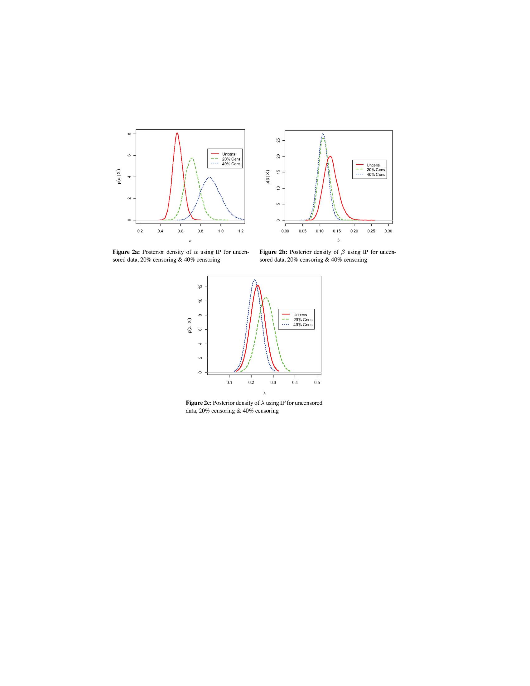
Figure 2 Marginal Posterior for complete and censored data using IP.

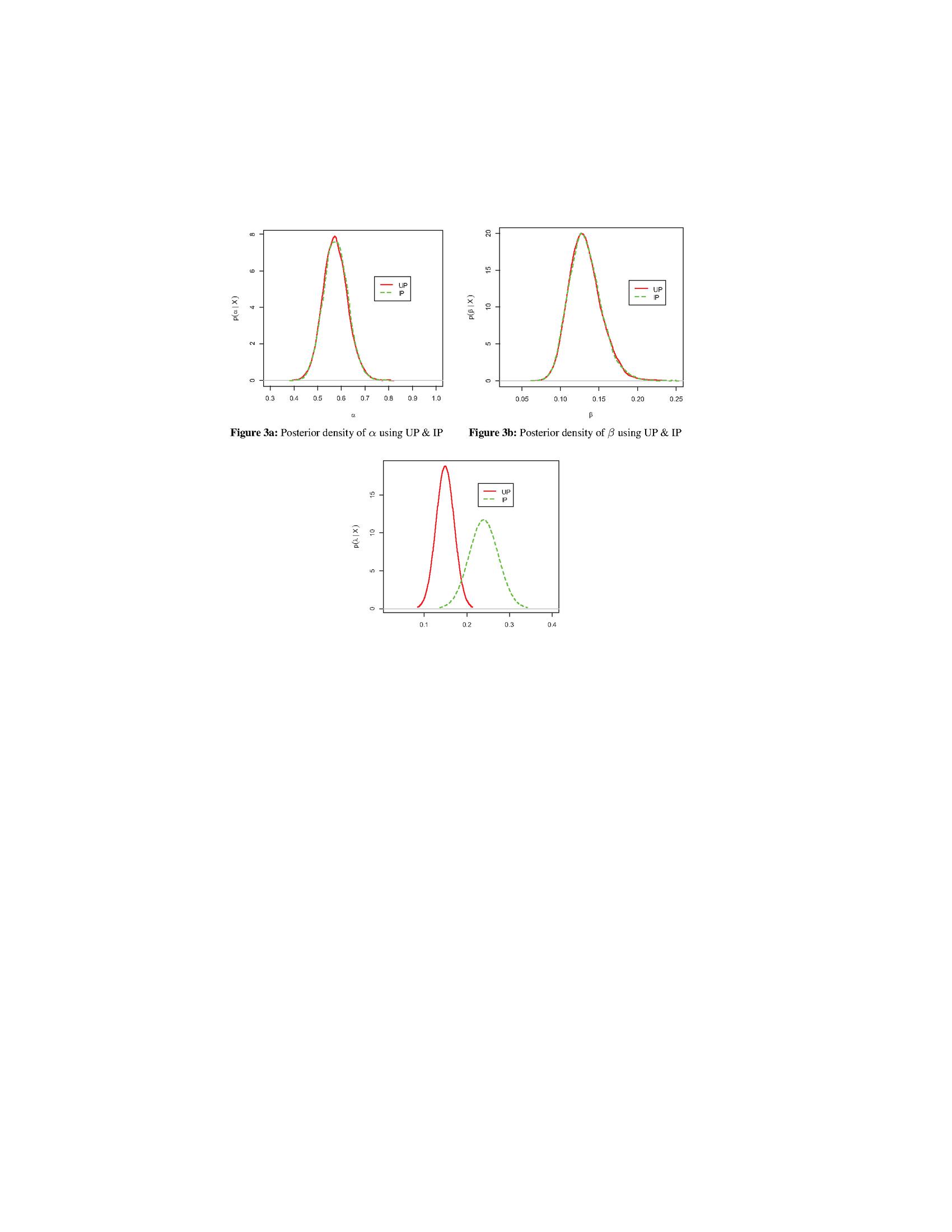
Figure 3 A comparison of marginal posteriors densities using informative and non-informative priors.

6.2 Tensile Fatigue Testing

Our second data set is about testing the tensile fatigue characteristics of polyester/viscose yarn to study the problem of warp breakage during weaving. The study consists of 100 centimeter yarn sampled at 2.3 percent strain level. This data set was studied by Queensberry et al. (1982), which is given as: 86, 364, 282, 40, 497, 55, 198, 146, 195, 224, 40,182, 61, 264, 251, 262, 149, 135, 423, 244, 105, 653, 88, 180, 597, 185, 20, 203, 98, 264, 325, 246, 229, 284, 124, 249, 157, 250, 211, 400, 393, 137, 400, 220, 196, 180, 338, 396, 135, 292, 42, 90, 93, 290, 203, 350, 131, 321, 229, 315, 398, 829,193, 169, 180, 166, 353, 71, 239, 188, 175, 198, 38, 571, 246, 236, 176, 38, 337, 124, 185 , 286,76, 20, 65, 279, 188,194, 264, 61, 151, 81, 568, 277, 15, 121, 341, 186, 55 and 143.

The transmuted Weibull distribution (2.1) is fitted to the data and the estimated parameters are given in Table 16.

Table 16 BEs and PRs of TWD with hyper parameters $a=0.5,b=1,c=1$ & $d=2$

	Loss Function	UP			IP
Data	$n$	$\alpha =2$	$\beta =1.2$	$\lambda =0.6$	$\alpha =2$	$\beta =1.2$	$\lambda =0.6$
Complete	SELF	2.1957 (0.0004)	1.0063 (0.0080)	0.5834 (0.0264)	2.1980 (0.0004)	1.0064 (0.0077)	0.5813 (0.0458)
	PLF	2.1967 (0.0019)	1.0072 (0.0018)	0.6056 (0.0444)	2.1989 (0.0019)	1.0072 (0.0017)	0.6195 (0.0763)
	QLF	2.1920 (0.0102)	1.0036 (0.2524)	0.5956 (0.0504)	2.1940 (0.0099)	1.0037 (0.2445)	0.6094 (0.0545)
20 %	SELF	2.2047 (0.0005)	1.0023 (0.0083)	0.5875 (0.0487)	2.2077 (0.0005)	1.0024 (0.0084)	0.5970 (0.0507)
Censoring	PLF	2.2060 (0.0025)	1.0027 (0.0027)	0.6276 (0.0802)	2.2090 (0.0025)	1.0027 (0.0019)	0.6381 (0.0821)
	QLF	2.1996 (0.0117)	1.0012 (0.3076)	0.6002 (0.0557)	2.2022 (0.0126)	1.0012 (0.2982)	0.6160 (0.0607)
40 %	SELF	2.2149 (0.0008)	1.0007 (0.0094)	0.6117 (0.0579)	2.2189 (0.0008)	1.0008 (0.0090)	0.6070 (0.0867)
Censoring	PLF	2.2170 (0.0035)	1.0008 (0.0031)	0.6029 (0.1611)	2.2206 (0.0035)	1.0009 (0.0030)	0.6746 (0.1335)
	QLF	2.2083 (0.0164)	1.0002 (0.4845)	0.6363 (0.0805)	2.2111 (0.0167)	1.0003 (0.4729)	0.6442 (0.0917)

Table 17 95% Bayesian Credible Intervals of TWD using UP and IP with hyper-parameters $a=0.5,b=1,c=1$ & $d=0.5$

		UP		IP
Data	Parameters	Lower Limit	Upper Limit	Lower Limit	Upper Limit
Complete	$𝜶=\text{𝟐}$	0.1825	2.2361	0.1843	2.2385
	$𝜷=\mathbf{\text{1.2}}$	0.0040	1.2153	0.0040	1.2148
	$𝝀=\mathbf{0.6}$	0.5512	0.9614	0.4256	1.0369
20% Censoring	$𝜶=\text{𝟐}$	0.1887	2.2519	0.1913	2.2554
	$𝜷=\mathbf{\text{1.2}}$	0.0043	1.2560	0.0064	1.2157
	$𝝀=\mathbf{0.6}$	0.5686	0.9724	0.5727	1.0585
40 % Censoring	$𝜶=\text{𝟐}$	0.1956	2.2738	0.1998	2.2771
	$𝜷=\mathbf{\text{1.2}}$	0.0048	1.2599	0.0143	1.2211
	$𝝀=\mathbf{0.6}$	0.0.5954	0.9826	0.5891	1.0763

In order to assess the goodness of fit data, we have computed p-value (0.271) by using the chi-square test to show that the data follow transmuted Weibull distribution at the 5% level of significance. It should be noted that the Bayes estimates, i.e., Table 16, of the scale and transmuted parameters are over-estimated while the shape parameter is under-estimated under the considered loss functions assuming the UP and the IP. From Table 17, it is noticed that the widths of 95% credible intervals decreased as the sample size increased.

7 Conclusion

In this article, Bayesian analysis of the transmuted Weibull distribution has been introduced assuming uniform and informative gamma priors under SELF, PLF and QLF. We conducted comprehensive simulations and real life studies to assess the relative performance of the Bayes estimators and also how to deal with the problems of selecting appropriate priors and loss functions at different sample sizes and test termination times under complete and censored data environments. In particular, we considered two different censoring rates, i.e., 20 and 40%. From Tables 2–10, it was noted that generally our results followed the consistency property of estimation, i.e., the Bayes estimates converge to the assumed parameter value by increasing the sample size. We also observed that the PRs for the censored data were larger than the uncensored data. Also, the widths of 95% credible intervals were observed decreased by increasing the sample size. Moreover, a same pattern has also been observed in the cases of real-life applications, which confirmed that the proposed MCMC algorithm is efficient to estimate the unknown parameters in the Bayesian framework. In future, one can extend the work using mixture of transmuted Weibull distribution (Aslam et al., 2020). Also, Bayesian analysis of record values using transmuted Weibull distribution may be considered.

References

[1] Abdurrahman, S.A. (2017). “Comparing Different Estimators of three Parameters for Transmuted Weibull Distribution”. Global Journal of Pure and Applied Mathematics. 13(9), 5115–5128.

[2] Ahmad, K., and Ahmad, S.P. (2015). “Structural Properties of Transmuted Weibull Distribution”.Journal of Modern Applied Statistical Methods. 14(2), 141–158.

[3] Afify, A. Z., Nofal, Z. M. and Ebraheim, A. N. (2015). “Exponentiated transmuted generalized Rayleigh distribution: a new four parameter Rayleigh distribution”. Pakistan Journal of Statistics and Operation Research, 11, 115–134.

[4] Ali, S. (2015). “On the Bayesian estimation of the weighted Lindley distribution”. Journal of Statistical Computation and Simulation, 85(5), 855–880.

[5] Ali, S., Aslam, M., and Kazmi, S.M.A. (2013). “Choice of Suitable Informative Prior for the Scale Parameter of the Mixture of Laplace Distribution”. Electronic Journal of Applied Statistical Analysis. 6, 32–56.

[6] Ali, S., Aslam, M., Nasir, A., and Kazmi, S.M.A. (May 2012). “Scale Parameter Estimation of the Laplace Model Using Different Asymmetric Loss Functions”. International Journal of Statistics and Probability, 1(1), 105–127.

[7] Al-Kadim, K.A., and Mohammed, M.H. (2017).“The Cubic Transmuted Weibull Distribution”. Journal of Babylon University: Pure and Applied Sciences, 3(25), 862–876.

[8] Aryal, G. R., and Tsokos, C. P. (2011). “Transmuted Weibull distribution: A generalization of the Weibull probability distribution”. European Journal of Pure and Applied Mathematics, 4(2), 89–102.

[9] Aslam, M., Kazmi, S.A.K., Ahmad, I., and Shah, S.H. (2014). “Bayesian Estimation for the Parameters of the Weibull Distribution”. Science International, 26(5), 1915–1920.

[10] Aslam, M., Ali, S., Yousaf, R., and Shah, I., (2020), “Mixture of transmuted Pareto distribution: Properties, applications and estimation under Bayesian framework”, Journal of the Franklin Institute , 357(5), 2934–2957.

[11] Cordeiro, G. M., Hashimoto, E. M., and Ortega, E. M. M. (2014). “The McDonald Weibull model, Statistics”. A Journal of Theoretical and Applied Statistics, 48, 256–278.

[12] Eberlya, L. E., and Casella, G. (2003). “Estimating Bayesian credible intervals”. Journal of Statistical Planning and Inference, 112, 115–132.

[13] Ebraheim, A.E.N. (2014). “Exponentiated Transmuted Weibull Distribution: A Generalization of the Weibull Distribution”. World Academy of Science, Engineering and Technology International Journal of Mathematical, Computational, Natural and Physical Engineering. 8(6), 897–905.

[14] Elbatal, I., &Aryal, G.R. (2013). “On the transmuted additive Weibull distribution”. Austrian Journal of Statistics, 42(2), 117–132.

[15] Gauss, C.F. (1810). “Least Squares method for the Combinations of Observations”. Translated by J. Bertrand 1955, Mallet-Bachelier, Paris.

[16] Gijbels, I. (2010). “Censored data”. Wiley Interdisciplinary Reviews: Computational Statistics, 2(2), 178–188.

[17] Kalbfleisch, J. D. and Prentice, R. L. (2011). “The statistical analysis of failure time data”. John Wiley & Sons Inc. New York.

[18] Khan, M.S., and King, R. (2013). “Transmuted Modified Weibull Distribution: A Generalization of the Modified Weibull Probability Distribution”. European Journal of pure and applied mathematics, 6(1), 66–88.

[19] Khan, M.S., and king, R., (2014). “Transmuted generalized inverse weibull distribution”. Journal of Applied Statistical Science. 20(3), 213–230.

[20] Khan, M.S., King, R., and Hudson, I.L. (2016). “Transmuted new generalized Weibull distribution for lifetime modeling”. Communications for Statistical Applications and Methods. 23(5), 363–383.

[21] Lawrence, J.D., Robert B. Gramacy, R.B., Thomas. L and Buckland, S.T. (2013). Methods in Ecology and Evolution, 4, 25–33.

[22] Lee, E.T., and Wang, J.W. (2003). Statistical Methods for Survival Data Analysis, Third ed. Wiley, New York.

[23] Mead, M. E. and Afify, A. Z. (2017). On five-parameter Burr XII distribution: Properties and Applications. South African Statistical Journal, 51, 67–80.

[24] Mendenhall, W. and Hader, R.A. (1958). “Estimation of parameters of mixed exponentially distributed failure time distributions from censored life test data”. Biometrika, 45, 504–520.

[25] Mobarak, M.A., Nofal, Z., and Mahdy, M. (2017). “On Size-Biased Weighted Transmuted Weibull Distribution”. International Journal of Advanced Research in Computer Science and Software Engineering. 7(3), 317–325.

[26] Mudholkar, G. Srivastava, D. and Kollia, G. (1996). “A generalization of the Weibull distribution with application to the analysis of survival data”. Journal of the American Statistical Association, 91(436), 1575–1583.

[27] Nofal, Z.M., and El Gebaly, Y.M. (2017. “Pakistan Journal of Statistics and Operation Research”. 8(2), 355–378.

[28] Norstrom, J. G. (1996). The use of precautionary loss functions in risk analysis. IEEE Transactions on Reliability, 45(1), 400–403.

[29] Punt, A. E., and Butterworth, D. S. (2000). “Why do Bayesian and maximum likelihood assessments of the Bering–Chukchi– Beaufort Seas stock of bowhead whales differ”? Journal of Cetacean Research and Management, 2, 125–133.

[30] Punt, A. E., and Walker, T. I. (1998). “Stock assessment and risk analysis for the school shark Galeorhinus galeus (Linnaeus) off southern Australia”. Marina and Freshwater Research, 49, 719–731.

[31] Queensberry, C. P., and Kent, J. (1982). “Selecting Among Probability Distributions Used in Reliability”. Technometrics, 24(1), 59–65.

[32] R Core Team (2013). R: A language and environment for statistical computing. R Foundation for Statistical Computing, Vienna, Austria. URL http://www.R-project.org/.

[33] Yousaf, R., Aslam, M., and Ali, S. (2018), Bayesian Estimation of the Transmuted Frèchet Distribution, Iranian Journal of Science and Technology, Transactions A: Science, DOI: 10.1007/s40995-018-0581-1.

[34] Romeu, L. J. (2004). “Censored data”, Strategic Arms Reduction Treaty. 11(3), 1–8.

[35] Shaw, W. T. and Buckley, I. R. C. (2009). “The alchemy of probability distributions: beyond Gram–Charlier expansions and a skew-kurtotic normal distribution from a rank transmutation map”. ArXiv Preprint: 0901.0434v1 [q-fin.ST].

[36] Tian, Y., Tian, M. and Zhu, Q. (2014). “Transmuted linear exponential distribution: A new generalization of the linear exponential distribution”. Communications in Statistics-Simulation and Computation, 43, 2661–2677.

Biographies

Rahila Yousaf recently completed her PhD in Statistics from Riphah International University, Islamabad. Her research interests are probability distributions and Bayesian inference.

Sajid Ali is an assistant professor at the Department of Statistics, Quaid-i-Azam University (QAU), Islamabad, Pakistan. He did his PhD in Statistics from Bocconi University, Milan, Italy. His research interest is focused on Bayesian inference, construction of new flexible probability distributions, and process monitoring.

Muhammad Aslam is a professor at the Riphah International University, Islamabad. Prior to this position, he served as a Professor and Chairman department of Statistics at Quaid-i-Azam University, Islamabad, Pakistan. He supervised more than 200 MPhil and 20 PhD students. He has published more than 150 articles in well reputed international journals. He completed his PhD from University of Wales, UK. His research interests are Bayesian inference, Paired comparison modelling and mathematical statistics.

Journal of Reliability and Statistical Studies, Vol. 13_2-4, 287–324.
doi: 10.13052/jrss0974-8024.13245
© 2020 River Publishers