Competing Hazards Regression Parameter Estimation Under Different Informative Priors

H. Rehman¹, N. Chandra^1,*, Fatemeh Sadat Hosseini-Baharanchi² and Ahmad Reza Baghestani³

¹Department of Statistics, Ramanujan School of Mathematical Sciences, Pondicherry University, Puducherry-605 014, India

²Minimally Invasive Surgery Research Center & Department of Biostatistics, School of Public Health, Iran University of Medical Sciences, Tehran, Iran

³Physiotherapy Research Center & Department of Biostatistics, Faculty of Paramedical Sciences, Shahid Beheshti University of Medical Sciences, Tehran, Iran

E-mail: rehmanh79@gmail.com; nc.stat@gmail.com; hosseini.fs@iums.ac.ir; baghestani.ar@gmail.com

*Corresponding Author

Received 01 July 2020; Accepted 18 November 2020; Publication 04 January 2021

Abstract

In the analysis of survival data, cause specific quantities of competing risks get considerable attention as compared to latent failure time approach. This article focuses on parametric regression analysis of survival data using cause specific hazard function with Burr type XII distribution as a baseline model. We obtained maximum likelihood and Bayes estimates of cumulative cause specific hazard functions under competing risk setup. For Bayesian point of view we proposed a class of informative priors for parameters to observe the comprehensive compatibility and their effectiveness under two different loss functions. The appropriateness of model is measured by the simulation study. Finally, we illustrate the proposed methodologies using bone marrow transplant data from the Princess Margaret Hospital Ontario, Canada.

Keywords: Competing risks, cause specific hazard, Cox regression, Burr type XII distribution, Bayes estimation, MCMC algorithm.

1 Introduction

The situation of competing risks occurs when the failure of individuals may be attributed to more than one causes of failure. The analysis of lifetime data in the presence of competing is based on two approaches, one is latent failure time approach and another is cause specific quantities. The former approach is not adequate in survival analysis because of its independence assumption is not verifiable in real life. In survival analysis, the cause specific quantities such as cumulative incidence function (CIF) and cause specific hazard function are popular because of their use and interpretation. Competing risks problem occurs in different fields such as medical sciences, engineering and social sciences. For example in bone marrow transplant when a patient goes for transplant, investigator is interested to observe the time to relapse, time to chronic graft versus host disease (CGVHD) and time to death. More detail on competing risk are available in (Beyersmann et al., 2012; Kalbfleisch and Prentice, 2002).

The cause specific hazard function $h_j(t)$ (Prentice et al., 1978) is defined the rate of failure due to cause $C\in \{1,2,\mathrm{\dots },p\}$ when the other causes also acting on the individuals. Mathematically it can be written as follows

$h_j(t|\mathbf{\text{X}})$	$=\underset{\mathrm{\Delta }t\to 0}{lim}\left\{{\displaystyle \frac{P(t\le T<t+\mathrm{\Delta }t,C=j|T>t,\mathbf{\text{X}})}{\mathrm{\Delta }t}}\right\};$
$j$	$=1,2,\mathrm{\dots },p.$	(1)

and formulation of CIF is given as,

$$F_j(t|\mathbf{\text{X}})=P(T\le t,C=j|\mathbf{\text{X}});j=1,2,\mathrm{\dots },p$$

(2)

where, the triplet $(T,C=j,\mathbf{\text{X}})$ represents the survival time, cause of failure and vector of explanatory variables related to subject/individual under study respectively. The quantity j is the realization of causes of failure. Mostly, medical sciences practitioners prefer to use semiparametric or nonparametric methods of survival analysis because they require less assumption compared to parametric methods. Parametric methods gives more precise result of the quantities of interest when they provide good fit to data (Lawless, 2014). In this article we consider parametric cause specific hazard regression model instead of semiparametric Cox proportional hazard regression model (Cox, 1972) by parameterizing the baseline cause specific hazard function.

In fact number of works based on classical parametric analysis of cause specific hazard function are cited in the literature. Benichou & Gail (1990) proposed the exponential or piecewise exponential model for estimating the CIF of event of interest. Bryant & Dignam (2004) are used constant cause specific hazard function for event of interest. Weibull cause specific hazard function is considered by Jeong & Fine (2006) for estimating CIF and compared with direct likelihood estimation of CIF by assuming the underlying time variable follow an improper Gompertz distribution. The idea of parametric reverse cause specific hazard function under left censoring is utilized by Anjana & Sankaran (2015) and they considered inverse Weibull distribution as a baseline model. Lee (2019) utilized the quantile method for estimating the CIF with the Weibull cause specific hazard function.

Most of the used distributions for modelling of cause specific hazard function are exponential and Weibull distributions. However, these distributions are capable to accommodate monotonically increasing or decreasing shape of the hazard function, they are incapable to analyse the nonmonotone behaviour of the hazard. In real life sometimes situation arise when the failure rates are not to be monotone, i.e., mortality reaches up to some extent or peak and then start slowly declines. So, in the light of these issues, we consider Burr type XII distribution (Burr, 1942; Gupta et al., 1996) as a baseline model for cause specific hazard function in Cox proportional hazards model. For the recent contribution on Burr type XII family of distribution one could refer to (Kehinde et al., 2018; Okasha and Shrahili, 2017).

In the context of Bayesian approach, Sen et al. (2010) considered Bayesian method of estimation for semiparametric survival analysis of breast cancer data with masked cause of failure. Sreedevi and Sankaran (2012) analysed the semiparametric cause specific hazard function through Bayesian approach by assuming gamma process prior for cumulative cause specific hazard function. Ge and Chen (2012) utilized the Bayesian method of estimation for fully specified subdistribution hazard model by considering piecewise exponential model with Jeffrey’s and gamma priors using Gibbs sampling algorithm. These are the very few works in literature revealed the Bayesian scenario pertaining to cause specific quantities in competing risks analysis.

The purpose of this article is to estimate the unknown parameters and cumulative cause specific hazard function through frequentist and Bayesian approach. For Bayesian point of view, we proposed a class of informative priors which consists Gamma, Weibull and lognormal priors for baseline parameters and standard normal prior for regression parameters under symmetric squared error loss function (SELF) (Sinha, 1998) as well as asymmetric LINEX loss function (LLF) (Soliman et al., 2006) for a comprehensive comparison study.

Recently, Burr type-XII distribution has attracted due to considerable amount of use in lifetime data analysis with respect to Bayesian estimation particularly for gamma informative prior. Soliman et al., (2011) considered the Bayesian analysis of the Burr type XII distribution based on record values. Byrnes et al., (2019) presented the Bayesian inference for the randomly censored Burr type XII distribution with the proportional hazards.

The key features of this article are as follows; we considered the competing risks analysis based on cause specific hazard approach because it completely determine competing risks process. Cause specific quantities provides the useful measure for observing the effect of covariates on different types of failure. We utilize the parametric model for the analysis of cause specific hazard function. Parametric models provide efficient and robust estimates if they correctly specified the data. We have employed both maximum likelihood and Bayesian methods for estimation of cumulative cause specific hazard function.

The rest of the article is organized is as follows. Section 2 deals with model formulation of Burr type XII cause specific hazard regression. We discuss the maximum likelihood and Bayesian method of estimation of cumulative cause specific hazard function in Section 3 and Section 4 respectively. To observe the finite sample behaviour of the model we conduct a simulation study in Section 5. Parametric cause specific hazard analysis is applied to the bone marrow transplant data in Section 6. Finally, Section 7 gives the conclusion of the study.

2 Model Formulation of Cause Specific Hazard Function

The Cox proportional hazards model can be extend in terms of cause specific hazard function by considering

$$h_j(t|\mathbf{\text{X}})=h_{0j}(t)\exp ({\mathit{\beta }}_j^{\prime }\mathbf{\text{X}}),j=1,2,\mathrm{\dots },p$$

(3)

where X is $m\times 1$ vector of covariates, ${\mathit{\beta }}_j$ is a $m\times 1$ vector of regression constants, $h_{oj}(t)$ is the baseline cause specific hazard rate and $h_j(t|\mathbf{\text{X}})$ is the cause specific hazard function in the presence of covariate X. For parameterizing the cause specific hazard function we assumed that baseline cause specific hazard corresponding to Burr type XII distribution as $h_{0j}(t,{\mathbf{\Theta }}_j)$ where, ${\mathbf{\Theta }}_j=({\alpha }_j,{\lambda }_j,a_j,{\mathit{\beta }}_j)$ is a vector of parameters. Therefore, cause specific hazard function, overall survival function and cumulative cause specific hazard function are obtained as follows

$$h_j(t|\mathbf{\text{X}})=\frac{{\alpha }_j{\lambda }_j{t}^{{\alpha }_j-1}{e}^{{\mathit{\beta }}_j^{\prime }\mathbf{\text{X}}}}{a_j{}^{{\alpha }_j}(1+{\left(\frac{t}{a_j}\right)}^{{\alpha }_j})},$$	(4)
$$S(t|\mathbf{\text{X}})=\exp (-\sum _{j=1}^p\log {[1+{\left(\frac{t}{a_j}\right)}^{{\alpha }_j}]}^{{\lambda }_j}{e}^{{\mathit{\beta }}_j^{\prime }\mathbf{\text{X}}}),$$	(5)
$$H_j(t|\mathbf{\text{X}})=\log {[1+{\left(\frac{t}{a_j}\right)}^{{\alpha }_j}]}^{{\lambda }_j}{e}^{{\mathit{\beta }}_j^{\prime }\mathbf{\text{X}}}$$	(6)

where ${\alpha }_j(>0)$ and ${\lambda }_j(>0)$ are shape parameters and $a_j(>0)$ is the scale parameter of the Burr type XII distribution. The above Figure 1 illustrate graphs of various shape of the density and hazard function of the Burr type XII distribution for the different values of the parameters.

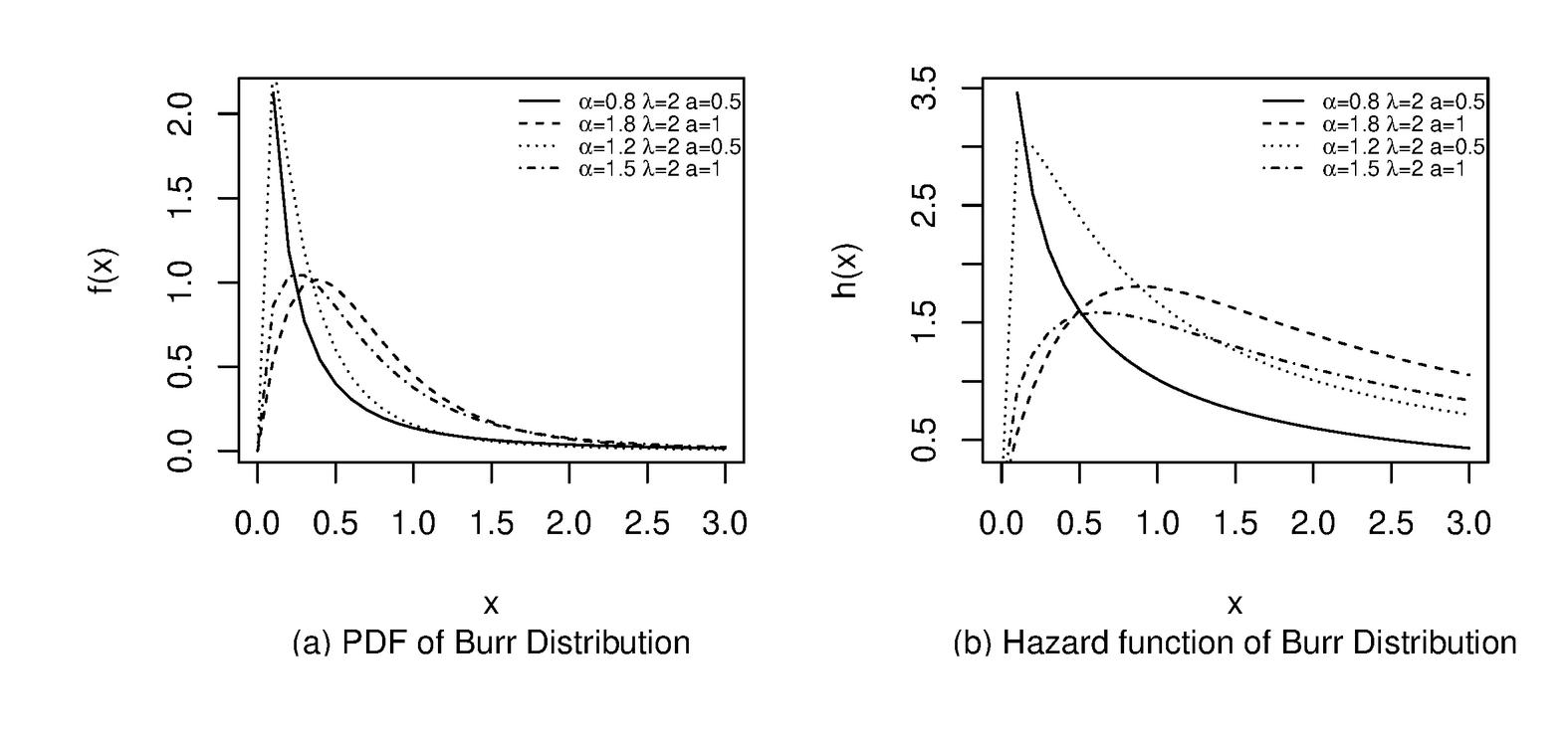
Figure 1 Probability density function (a) and hazard function (b).

3 Maximum Likelihood (ML) Estimation

We now determine the parameter estimation of cause specific hazard approach through maximum likelihood estimation. Let we have $n\in \mathbb{N}$ independent random samples of $(t_i,j_i,{\delta }_i,{\mathbf{\text{X}}}_i)$, $i=1,2,\mathrm{\dots },n$ of individuals. Define $T_i=\min (T_i^{*},D_i)$, $T_i^{*}\in {ℝ}^{+}$, where $T_i^{*}$ and $D_i$ are the failure time and censoring time, respectively. We assume that the censoring and failure times are independent. The indicator variable ${\delta }_i=0$ or 1, it takes value 0 when individual is censored and 1 when individual die due to cause j. A likelihood function based on cause specific hazard function is given as

$$L(\mathbf{\Theta })=\prod _{i=1}^n\left(\prod _{j=1}^p{h}_j{\left(t_i|{\mathbf{\text{X}}}_i\right)}^{{\delta }_i}S(t_i|{\mathbf{\text{X}}}_i)\right)$$

(7)

where $\mathbf{\Theta }=({\mathbf{\Theta }}_1,{\mathbf{\Theta }}_2,\mathrm{\dots },{\mathbf{\Theta }}_p)$, $j=1,2,\mathrm{\dots },p$. Now the likelihood function under Burr type XII cause specific hazard function is obtained as follows

$L({\mathit{t}}_i,{\mathbf{\text{X}}}_i|{\alpha }_j,{\lambda }_j,a_j,{\mathit{\beta }}_j)$
$\mathrm{\hspace{1em}\hspace{1em}}={\displaystyle \prod _{i=1}^n}{\displaystyle \prod _{j=1}^p}{\left({\alpha }_j{\lambda }_j{a}_j{}^{-{\alpha }_j}t_i^{{\alpha }_j-1}{\left(1+{\left({\displaystyle \frac{t_i}{a_j}}\right)}^{{\alpha }_j}\right)}^{-1}{e}^{{\mathit{\beta }}_j^{\prime }{\mathbf{\text{X}}}_i}\right)}^{{\delta }_i}$
$\mathrm{\hspace{1em}\hspace{1em}}\mathit{\hspace{1em}}\times \exp (-{\displaystyle \sum _{j=1}^p}{\lambda }_j\log [1+{\left({\displaystyle \frac{t_i}{a_j}}\right)}^{{\alpha }_j}]e^{{\mathit{\beta }}_j^{\prime }{\mathbf{\text{X}}}_i}).$	(8)

The log likelihood function is given as

$l$	$={\displaystyle \sum _{j=1}^p}{n}_j\log {\alpha }_j+{\displaystyle \sum _{j=1}^p}{n}_j\log {\lambda }_j-{\displaystyle \sum _{j=1}^p}{n}_j{\alpha }_j\log a_j+{\displaystyle \sum _{j=1}^p}({\alpha }_j-1){\displaystyle \sum _{i=1}^{n_j}}\log t_i$
	$\mathrm{\hspace{1em}}-{\displaystyle \sum _{j=1}^p}{\displaystyle \sum _{i=1}^{n_j}}\log \left(1+{\left({\displaystyle \frac{t_i}{a_j}}\right)}^{{\alpha }_j}\right)+{\displaystyle \sum _{j=1}^p}{\displaystyle \sum _{i=1}^{n_j}}{\mathit{\beta }}_j^{\prime }{\mathbf{\text{X}}}_i$
	$\mathrm{\hspace{1em}}-{\displaystyle \sum _{i=1}^n}{\displaystyle \sum _{j=1}^p}{\lambda }_j\log \left(1+{\left({\displaystyle \frac{t_i}{a_j}}\right)}^{{\alpha }_j}\right)e^{{\mathit{\beta }}_j^{\prime }{\mathbf{\text{X}}}_i}.$	(9)

The likelihood equations for the parameters ${\alpha }_j,{\lambda }_j,a_j$ and ${\mathit{\beta }}_j$ are obtained as

${\displaystyle \frac{\partial l}{\partial {\alpha }_j}}$	$={\displaystyle \frac{n_j}{{\alpha }_j}}-n_j\log a_j+{\displaystyle \sum _{i=1}^{n_j}}\log t_i-{\displaystyle \sum _{i=1}^{n_j}}{\displaystyle \frac{{\left(\frac{t_i}{a_j}\right)}^{{\alpha }_j}\log \frac{t_i}{a_j}}{1+{\left(\frac{t_i}{a_j}\right)}^{{\alpha }_j}}}$
	$\mathrm{\hspace{1em}}-{\displaystyle \sum _{i=1}^n}{\displaystyle \frac{{\lambda }_j{\left(\frac{t_i}{a_j}\right)}^{{\alpha }_j}\log \left(\frac{t_i}{a_j}\right)}{1+{\left(\frac{t_i}{a_j}\right)}^{{\alpha }_j}}}{e}^{{\mathit{\beta }}_j^{\prime }{\mathbf{\text{X}}}_i}=0$	(10)
${\displaystyle \frac{\partial l}{\partial {\lambda }_j}}$	$={\displaystyle \frac{n_j}{{\lambda }_j}}-{\displaystyle \sum _{i=1}^n}\log \left(1+{\left({\displaystyle \frac{t_i}{a_j}}\right)}^{{\alpha }_j}\right)e^{{\mathit{\beta }}_j^{\prime }{\mathbf{\text{X}}}_i}=0$	(11)
${\displaystyle \frac{\partial l}{\partial a_j}}$	$=-{\displaystyle \frac{n_j{\alpha }_j}{a_j}}+{\displaystyle \sum _{i=1}^{n_j}}{\displaystyle \frac{{\alpha }_j{t}_i^{{\alpha }_j}}{\left(1+{\left(\frac{t_i}{a_j}\right)}^{{\alpha }_j}\right)a_j^{{\alpha }_j+1}}}$
	$\mathrm{\hspace{1em}}+{\displaystyle \sum _{i=1}^n}{\displaystyle \frac{{\alpha }_j{\lambda }_j{t}_i^{{\alpha }_j}{e}^{{\mathit{\beta }}_j^{\prime }{\mathbf{\text{X}}}_i}}{\left(1+{\left(\frac{t_i}{a_j}\right)}^{{\alpha }_j}\right)a_j^{{\alpha }_j+1}}}=0$	(12)
${\displaystyle \frac{\partial l}{\partial {\mathit{\beta }}_j}}$	$={\displaystyle \sum _{i=1}^{n_j}}{\mathbf{\text{X}}}_i-{\displaystyle \sum _{i=1}^n}{\lambda }_j{\mathbf{\text{X}}}_i\log \left(1+{\left({\displaystyle \frac{t_i}{a_j}}\right)}^{{\alpha }_j}\right)e^{{\mathit{\beta }}_j^{\prime }{\mathbf{\text{X}}}_i}=0.$	(13)

It is realized that the likelihood equations (3)–(13) are not in explicit form and cannot be solved analytically. The maximum likelihood estimate of the parameters are determined by using numerical method. Standard error of the parameters is the square root of the diagonal element of variance covariance matrix which is nothing but the inverse of Fisher information matrix. Whereas, the $\widehat{\mathbf{\Theta }}\sim N(\mathbf{\Theta },I^{-1}(\mathbf{\Theta }))$ asymptotically and Fisher information matrix is given by

$$I(\mathbf{\Theta })=-E\left(\begin{array}{ccc}\hfill \frac{{\partial }^{2}l}{\partial {\alpha }_j^2}\mathit{\hspace{1em}}\hfill & \hfill \mathrm{\dots }\mathit{\hspace{1em}}\hfill & \hfill \frac{{\partial }^{2}l}{\partial {\alpha }_j\partial {\mathit{\beta }}_j}\hfill \\ \hfill \mathrm{⋮}\mathit{\hspace{1em}}\hfill & \hfill \mathrm{\ddots }\mathit{\hspace{1em}}\hfill & \hfill \mathrm{⋮}\hfill \\ \hfill \frac{{\partial }^{2}l}{\partial {\mathit{\beta }}_j\partial {\alpha }_j}\mathit{\hspace{1em}}\hfill & \hfill \mathrm{\cdots }\mathit{\hspace{1em}}\hfill & \hfill \frac{{\partial }^{2}l}{\partial {\mathit{\beta }}_j^2}\hfill \end{array}\right).$$

Once the parameters estimates are obtained, the cumulative cause specific hazard estimates can be obtained through invariance property of ML estimates in equation (6) as follows

$${\widehat{H}}_j(t|\mathbf{\text{X}})=\log {[1+{\left(\frac{t}{{\widehat{a}}_j}\right)}^{{\widehat{\alpha }}_j}]}^{{\widehat{\lambda }}_j}{e}^{{\widehat{\mathit{\beta }}}_j^{\prime }\mathbf{\text{X}}}.$$

4 Bayesian Method of Estimation

In this section we provide the Bayes estimates of cumulative cause specific hazard function under two different loss function. We proposed a class of informative priors, which consists gamma, Weibull and lognornal distributions. We assume, ${\alpha }_j,{\lambda }_j$ and $a_j$ are independent random variables having the gamma density i.e. ${\alpha }_j\sim G(q_{{\alpha }_j},r_{{\alpha }_j}),{\lambda }_j\sim G(q_{{\lambda }_j},r_{{\lambda }_j})$ and $a_j\sim G(q_{a_j},r_{a_j})$. The random variable ${\mathit{\beta }}_j$ is assumed to follow a standard normal distribution i.e. ${\mathit{\beta }}_j\sim N(0,1).$ Therefore, the joint prior distribution of ${\alpha }_j,{\lambda }_j,a_j$ and ${\mathit{\beta }}_j$ is equivalent to

${\pi }_1({\alpha }_j,{\lambda }_j,a_j,{\mathit{\beta }}_j)\propto {\alpha }_j^{q_{{\alpha }_j}-1}{\lambda }_j^{q_{{\lambda }_j}-1}{a}_j^{q_{a_j}-1}{e}^{-\left(r_{{\alpha }_j}{\alpha }_j+r_{{\lambda }_j}{\lambda }_j+r_{a_j}{a}_j+\frac{1}{2}{\mathit{\beta }}_j^2\right)};$
$\mathrm{\hspace{1em}\hspace{1em}}({\alpha }_j,{\lambda }_j,a_j)>0,-\mathrm{\infty }<{\mathit{\beta }}_j<\mathrm{\infty },$	(14)

where $q$ and $r$are positive hyper-parameters respect to ${\alpha }_j,{\lambda }_j$ and $a_j$ which will responsible for the prior knowledge of the parameters. Now the joint posterior distribution of the random variables ${\alpha }_j,{\lambda }_j,a_j$ and ${\mathit{\beta }}_j$ given the observed data ${\mathit{t}}_i,{\mathbf{\text{X}}}_i$ obtained by

$p_1({\alpha }_j,{\lambda }_j,a_j,{\mathit{\beta }}_j|{\mathit{t}}_i,{\mathbf{\text{X}}}_i)\propto {\alpha }_j^{n_j+q_{{\alpha }_j}-1}{\lambda }_j^{n_j+q_{{\lambda }_j}-1}{a}_j^{n_j{\alpha }_j+q_{a_j}-1}{\displaystyle \prod _{i=1}^{n_j}}{t}_i^{{\alpha }_j-1}$
$\mathrm{\hspace{1em}}\times {\left(1+{\left({\displaystyle \frac{t_i}{a_j}}\right)}^{{\alpha }_j}\right)}^{-1}{e}^{{\sum }_{j=1}^p{\sum }_{i=1}^{n_j}{\mathit{\beta }}_j^{\prime }{\mathbf{\text{X}}}_i}$
$\mathrm{\hspace{1em}}\times e^{-\left({\sum }_{i=1}^n{\sum }_{j=1}^p{\lambda }_j\log \left[1+{\left(\frac{t_i}{a_j}\right)}^{{\alpha }_j}\right]e^{{\mathit{\beta }}_j^{\prime }{\mathbf{\text{X}}}_i}\right)}$
$\mathrm{\hspace{1em}}\times e^{-\left(r_{{\alpha }_j}{\alpha }_j+r_{{\lambda }_j}{\lambda }_j+r_{a_j}{a}_j+\frac{1}{2}{\mathit{\beta }}_j^2\right)}.$	(15)

Similarly, we assumed the Weibull and lognormal priors for baseline parameters and standard normal prior for regression parameters. Then the joint prior distributions of the random variables are obtained as follows

${\pi }_2({\alpha }_j,{\lambda }_j,a_j,{\mathit{\beta }}_j)$	$\propto {\alpha }_j^{k_{{\alpha }_j}-1}{\lambda }_j^{k_{{\lambda }_j}-1}{a}_j^{k_{a_j}-1}$
	$\mathrm{\hspace{1em}}\times e^{-\left({\left({\theta }_{{\alpha }_j}{\alpha }_j\right)}^{k_{{\alpha }_j}}+{({\theta }_{{\lambda }_j}{\lambda }_j)}^{k_{{\lambda }_j}}+{({\theta }_{a_j}{a}_j)}^{k_{a_j}}+\frac{1}{2}{\mathit{\beta }}_j^2\right)};$
	$\mathrm{\hspace{1em}}\times ({\alpha }_j,{\lambda }_j,a_j)>0,-\mathrm{\infty }<{\mathit{\beta }}_j<\mathrm{\infty },$	(16)
${\pi }_2({\alpha }_j,{\lambda }_j,a_j,{\mathit{\beta }}_j)$	$\propto {\displaystyle \frac{1}{{\alpha }_j{\lambda }_j{a}_j}}$
	$\mathrm{\hspace{1em}}\times e^{-\frac{1}{2}\left({\left(\frac{\log {\alpha }_j-{\mu }_{{\alpha }_j}}{{\sigma }_{{\alpha }_j}}\right)}^2+{\left(\frac{\log {\lambda }_j-{\mu }_{{\lambda }_j}}{{\sigma }_{{\lambda }_j}}\right)}^2+{\left(\frac{\log a_j-{\mu }_{a_j}}{{\sigma }_{a_j}}\right)}^2+\frac{1}{2}{\mathit{\beta }}_j^2\right)};$
	$\mathrm{\hspace{1em}}({\alpha }_j,{\lambda }_j,a_j)>0,-\mathrm{\infty }<{\mathit{\beta }}_j<\mathrm{\infty },$	(17)

where $(k,\theta )>0,-\mathrm{\infty }<\mu <\mathrm{\infty }$ and $\sigma >0$ are the hyper-parameters. Thus, the joint posterior distributions of the random variables ${\alpha }_j,{\lambda }_j,a_j$ and ${\mathit{\beta }}_j$ under the above joint prior distributions (4) and (17) turn out to have the following forms.

$p_2({\alpha }_j,{\lambda }_j,a_j,{\mathit{\beta }}_j|{\mathit{t}}_i,{\mathbf{\text{X}}}_i)$
$\mathrm{\hspace{1em}\hspace{1em}}\propto {\alpha }_j^{n_j+k_{{\alpha }_j}-1}{\lambda }_j^{n_j+k_{{\lambda }_j}-1}{a}_j^{n_j{\alpha }_j+k_{a_j}-1}$
$\mathrm{\hspace{1em}\hspace{1em}}\mathit{\hspace{1em}}\times {\displaystyle \prod _{i=1}^{n_j}}{t}_i^{{\alpha }_j-1}{(1+{\left({\displaystyle \frac{t_i}{a_j}}\right)}^{{\alpha }_j})}^{-1}{e}^{{\sum }_{j=1}^p{\sum }_{i=1}^{n_j}{\mathit{\beta }}_j^{\prime }{\mathbf{\text{X}}}_i}$
$\mathrm{\hspace{1em}\hspace{1em}}\mathit{\hspace{1em}}\times e^{-\left({\sum }_{i=1}^n{\sum }_{j=1}^p{\lambda }_j\log \left[1+{\left(\frac{t_i}{a_j}\right)}^{{\alpha }_j}\right]e^{{\mathit{\beta }}_j^{\prime }{\mathbf{\text{X}}}_i}\right)}$
$\mathrm{\hspace{1em}\hspace{1em}}\mathit{\hspace{1em}}\times e^{-\left({\left({\theta }_{{\alpha }_j}{\alpha }_j\right)}^{k_{{\alpha }_j}}+{({\theta }_{{\lambda }_j}{\lambda }_j)}^{k_{{\lambda }_j}}+{({\theta }_{a_j}{a}_j)}^{k_{a_j}}+\frac{1}{2}{\mathit{\beta }}_j^2\right)},$	(18)
$p_3({\alpha }_j,{\lambda }_j,a_j,{\mathit{\beta }}_j|{\mathit{t}}_i,{\mathbf{\text{X}}}_i)$
$\mathrm{\hspace{1em}\hspace{1em}}\propto {\alpha }_j^{n_j-1}{\lambda }_j^{n_j-1}{a}_j^{n_j{\alpha }_j-1}$
$\mathrm{\hspace{1em}\hspace{1em}}\mathit{\hspace{1em}}\times {\displaystyle \prod _{i=1}^n}{t}_i^{{\alpha }_j-1}{(1+{\left({\displaystyle \frac{t_i}{a_j}}\right)}^{{\alpha }_j})}^{-1}{e}^{{\sum }_{j=1}^p{\sum }_{i=1}^{n_j}{\mathit{\beta }}_j^{\prime }{\mathbf{\text{X}}}_i}$
$\mathrm{\hspace{1em}\hspace{1em}}\mathit{\hspace{1em}}\times e^{-\left({\sum }_{i=1}^n{\sum }_{j=1}^p{\lambda }_j\log \left[1+{\left(\frac{t_i}{a_j}\right)}^{{\alpha }_j}\right]e^{{\mathit{\beta }}_j^{\prime }{\mathbf{\text{X}}}_i}\right)}$
$\mathrm{\hspace{1em}\hspace{1em}}\mathit{\hspace{1em}}\times e^{-\frac{1}{2}\left({\left(\frac{\log {\alpha }_j-{\mu }_{{\alpha }_j}}{{\sigma }_{{\alpha }_j}}\right)}^2+{\left(\frac{\log {\lambda }_j-{\mu }_{{\lambda }_j}}{{\sigma }_{{\lambda }_j}}\right)}^2+{\left(\frac{\log a_j-{\mu }_{a_j}}{{\sigma }_{a_j}}\right)}^2+\frac{1}{2}{\mathit{\beta }}_j^2\right)}.$	(19)

It is observed under each assumed priors, the joint posterior densities in equations (4), (4) and (4) are not in any explicit form and cannot be solved analytically. So, it is difficult to obtain marginal posterior densities due to ratio of multiple integrals. Therefore, as an alternative, numerical approximation algorithm such as Markov Chain Monte Carlo (MCMC) (Robert et al. (2010)) have been used to evaluate the expressions. Next, we obtained the Bayes estimates of cumulative cause specific hazard function under SELF as well as LLF. Thus, the Bayes estimates of cumulative cause specific hazard function $H_j(t|\mathbf{\text{X}})$ from equation (6), using the considered priors, under SELF and LLF are respectively, given by

${\widehat{H}}_j^{self}(t|\mathbf{\text{X}})$	$={\displaystyle \frac{1}{N}}{\displaystyle \sum _{l=1}^N}{[{\widehat{H}}_j(t|\mathbf{\text{X}})]}_{{\alpha }_j={\alpha }_l,{\lambda }_j={\lambda }_l,a_j=a_l,{\mathit{\beta }}_j={\mathit{\beta }}_l},$
${\widehat{H}}_j^{llf}(t|\mathbf{X})$	$=-{\displaystyle \frac{1}{p}}\log \left({\displaystyle \frac{1}{N}}{\displaystyle \sum _{l=1}^N}{e}^{-p{[{\widehat{H}}_j(t|\mathbf{X})]}_{{\alpha }_j={\alpha }_l,{\lambda }_j={\lambda }_l,a_j=a_l,{\mathit{\beta }}_j={\mathit{\beta }}_l}}\right)$

where ${\alpha }_l,{\lambda }_l,a_l$ and ${\mathit{\beta }}_l$, $l=1,2,\mathrm{\dots },N$ are the random sample drawn from the marginal posterior distributions of ${\alpha }_j,{\lambda }_j,a_j$ and ${\mathit{\beta }}_j$ respectively through MCMC algorithm and, $p$ is the hyper-parameter of LLF which is assumed to be known.

5 Simulation Study

We performed Monte Carlo simulation study to observe the finite sample behaviour of the proposed estimates of cumulative cause specific hazard function. We consider different choice of sample size n such as $n=20$, 50, 100 and 200. For the sack of simplicity, we considered two causes of failure i.e. $j=1$, 2 and one single covariate X. Comparison of estimates are made on the basis of average estimate and empirical mean square error (MSE) of cumulative cause specific hazard function of both the causes. The whole process is repeated 500 times.

For generating the survival time form Burr type XII distribution through inverse transformation, we adopt the procedure given in Beyersmann et al. (2012). Let the true values of model parameter are given as ${\alpha }_1=1.5$, ${\lambda }_1=1.6,a_1=5,{\beta }_1=0.1$ and ${\alpha }_2=1.7,{\lambda }_2=1.6,a_2=7,{\beta }_2=0.2$ for cause 1 and cause 2 respectively. The covariate X is generated from standard normal distribution. Further, we generate the two causes of failure from the binomial distribution. The censoring time D${}_i$ is generated from $U(0,d_i)$, where d${}_i$ is imposing the percentage of censoring around 20%. We assume that parameter $a_j$ is known for mathematically convenient while estimating the parameters.

ML estimates and standard error of the unknown parameter ${\alpha }_j,{\lambda }_j,a_j$ and ${\beta }_j$ are obtained based on log likelihood function in equation (3) through optim function in R. Invariance property of ML estimate is utilized for obtaining the estimates of cumulative cause specific hazard function. It is noticed that the expressions of joint posterior densities under considered informative priors are not in explicit form and cannot be solved analytically and the marginal posterior also not obtained. In such situations the well known MCMC techniques namely, Gibbs sampling (Geman and Geman, 1984), Metropolis–Hastings algorithm (Hastings, 1970) etc. are popular for generating the posterior samples. Therefore, we used BUGS software in R through OpenBUGS interface (Lunn et al., 2012) for drawing the MCMC samples.

The hyper-parameters of the assumed informative priors are calculated based on 1,000 random samples. Now, for each considered sample, first we obtain the ML estimate of each parameter and compute the mean and empirical variance and compare with the mean and variance of assumed priors. Calculated hyper-parameters of gamma, Weibull and lognormal priors given below.

Priors	Parameters
Gamma	$q_{{\alpha }_1}=41.64,r_{{\alpha }_1}=26.57,q_{{\lambda }_1}=20.26,r_{{\lambda }_1}=12.17$,
	$q_{{\alpha }_2}=27.52,r_{{\alpha }_2}=15.43,q_{{\lambda }_2}=9.41,r_{{\lambda }_2}=5.5$
Weibull	$k_{{\alpha }_1}=7.64,{\theta }_{{\alpha }_1}=0.02,k_{{\lambda }_1}=5.17,{\theta }_{{\lambda }_1}=0.05$,
	$k_{{\alpha }_2}=6.11,{\theta }_{{\alpha }_2}=0.02,k_{{\lambda }_2}=3.39,{\theta }_{{\lambda }_2}=0.11$
Lognormal	${\mu }_{{\alpha }_1}=0.44,{\sigma }_{{\alpha }_1}=0.02,{\mu }_{{\lambda }_1}=0.49,{\sigma }_{{\lambda }_1}=0.05$,
	${\mu }_{{\alpha }_2}=0.56,{\sigma }_{{\alpha }_2}=0.04,{\mu }_{{\lambda }_2}=0.49,{\sigma }_{{\lambda }_2}=0.01$

Table 1 ML, Bayes estimates and their MSEs for cumulative cause specific hazard function for cause-1 and cause-2 with $n=20$ at $X=-0.3$ when ${\alpha }_1=1.5,{\lambda }_1=1.6,a_1=5,{\beta }_1=0.1$, ${\alpha }_2=1.7,{\lambda }_2=1.6,a_2=7,{\beta }_2=0.2$

$n=20$		Cause 1			Cause 2
Time Points		0.5	1	1.5	0.5	1	1.5
True Value		0.04834	0.13302	0.23622	0.01687	0.05415	0.10602
ML	Estimate	0.05338	0.14087	0.25164	0.01769	0.05081	0.09756
	MSE	0.18103	0.75786	1.81967	0.03872	0.19796	0.54976
Gamma	Estimate	0.05144	0.13837	0.24541	0.01844	0.05563	0.10712
SELF	MSE	0.02797	0.1228	0.28261	0.008	0.04601	0.12638
Gamma $p=1.5$	Estimate	0.05099	0.13663	0.24175	0.01829	0.05491	0.10533
LLF	MSE	0.02702	0.11705	0.26574	0.00778	0.04419	0.12058
Gamma	Estimate	0.05191	0.14018	0.24926	0.01859	0.05638	0.10903
LLF $p=-1.5$	MSE	0.02900	0.12956	0.30365	0.00824	0.04808	0.13344
Weibull	Estimate	0.05071	0.13636	0.24232	0.01868	0.05598	0.10775
SELF	MSE	0.03322	0.13158	0.28777	0.00995	0.0512	0.13392
Weibull	Estimate	0.05018	0.13452	0.23865	0.01849	0.05518	0.10587
LLF $p=1.5$	MSE	0.03166	0.12444	0.2713	0.00954	0.04852	0.12633
Weibull	Estimate	0.05126	0.13829	0.24619	0.01887	0.05682	0.10976
LLF $p=-1.5$	MSE	0.03498	0.14016	0.30872	0.01039	0.05431	0.14325
Lognormal	Estimate	0.05064	0.13759	0.24503	0.01874	0.05612	0.10759
SELF	MSE	0.02231	0.10637	0.25872	0.00846	0.048	0.13029
Lognormal	Estimate	0.05025	0.136	0.24155	0.0186	0.05539	0.10578
LLF $p=1.5$	MSE	0.02168	0.10171	0.24287	0.00823	0.04614	0.1244
Lognormal	Estimate	0.05103	0.13924	0.24867	0.01889	0.05688	0.1095
LLF $p=-1.5$	MSE	0.02301	0.11186	0.27844	0.0087	0.0501	0.13746

Table 2 ML, Bayes estimates and their MSEs for cumulative cause specific hazard function for cause-1 and cause-2 with $n=50$ at $X=-0.3$ when ${\alpha }_1=1.5,{\lambda }_1=1.6,a_1=5,{\beta }_1=0.1,{\alpha }_2=1.7,{\lambda }_2=1.6,a_2=7,{\beta }_2=0.2$

$n=50$		Cause 1			Cause 2
Time Points		0.5	1	1.5	0.5	1	1.5
True Value		0.04834	0.13302	0.23622	0.01687	0.05415	0.10602
ML	Estimate	0.0525	0.14117	0.25051	0.01737	0.05376	0.1053
	MSE	0.07667	0.31333	0.71655	0.01538	0.08362	0.22294
Gamma	Estimate	0.05125	0.13834	0.24525	0.01785	0.05502	0.10683
SELF	MSE	0.02759	0.12129	0.27994	0.00641	0.03849	0.10789
Gamma	Estimate	0.05097	0.13728	0.24306	0.01777	0.05461	0.10581
LLF $p=1.5$	MSE	0.02702	0.1179	0.27025	0.00631	0.03767	0.1052
Gamma	Estimate	0.05154	0.13943	0.2475	0.01793	0.05543	0.10788
LLF $p=-1.5$	MSE	0.02819	0.12503	0.29101	0.00651	0.03937	0.11094
Weibull	Estimate	0.04986	0.13555	0.24163	0.01748	0.05437	0.10629
SELF	MSE	0.03036	0.12549	0.28064	0.0067	0.03885	0.10758
Weibull	Estimate	0.04956	0.13448	0.23948	0.0174	0.05396	0.10528
LLF $p=1.5$	MSE	0.02964	0.12197	0.27214	0.00658	0.03793	0.10469
Weibull	Estimate	0.05016	0.13666	0.24384	0.01757	0.0548	0.10734
LLF $p=-1.5$	MSE	0.03113	0.12942	0.29046	0.00682	0.03985	0.11085
Lognormal	Estimate	0.0507	0.13773	0.24478	0.01816	0.05555	0.10738
SELF	MSE	0.02338	0.10906	0.26163	0.00665	0.03915	0.1082
Lognormal	Estimate	0.05045	0.13674	0.24268	0.01808	0.05514	0.10636
LLF $p=1.5$	MSE	0.02297	0.10626	0.2527	0.00655	0.03831	0.1055
Lognormal	Estimate	0.05096	0.13874	0.24693	0.01824	0.05597	0.10844
LLF $p=-1.5$	MSE	0.02382	0.11216	0.27183	0.00675	0.04004	0.11124

Table 3 ML, Bayes estimates and their MSEs for cumulative cause specific hazard function for cause-1 and cause-2 with $n=100$ at $X=-0.3$ when ${\alpha }_1=1.5,{\lambda }_1=1.6,a_1=5,{\beta }_1=0.1$, ${\alpha }_2=1.7,{\lambda }_2=1.6,a_2=7,{\beta }_2=0.2$

$n=100$		Cause 1			Cause 2
Time Points		0.5	1	1.5	0.5	1	1.5
True Value		0.04834	0.13302	0.23622	0.01687	0.05415	0.10602
ML	Estimate	0.05072	0.13839	0.24626	0.01811	0.05595	0.10846
	MSE	0.03659	0.15759	0.37248	0.0098	0.0509	0.12839
Gamma	Estimate	0.05043	0.13727	0.24397	0.01799	0.05555	0.10764
SELF	MSE	0.02081	0.09377	0.22189	0.00556	0.0314	0.08356
Gamma	Estimate	0.05026	0.13663	0.24266	0.01794	0.05531	0.10704
LLF $p=1.5$	MSE	0.02055	0.0922	0.21722	0.00551	0.03098	0.08227
Gamma	Estimate	0.0506	0.13792	0.2453	0.01804	0.0558	0.10825
LLF $p=-1.5$	MSE	0.02107	0.09546	0.22702	0.00561	0.03184	0.08496
Weibull	Estimate	0.04905	0.13478	0.24104	0.01753	0.05469	0.10674
SELF	MSE	0.02159	0.09428	0.21832	0.00571	0.03183	0.08414
Weibull	Estimate	0.04888	0.13414	0.23975	0.01748	0.05444	0.10614
LLF $p=1.5$	MSE	0.02132	0.09283	0.21442	0.00565	0.03139	0.08281
Weibull	Estimate	0.04922	0.13544	0.24236	0.01758	0.05494	0.10735
LLF $p=-1.5$	MSE	0.02187	0.09585	0.22265	0.00577	0.03229	0.08559
Lognormal	Estimate	0.05008	0.13678	0.24342	0.01826	0.05602	0.10813
SELF	MSE	0.01861	0.08721	0.21198	0.0058	0.03208	0.084
Lognormal	Estimate	0.04993	0.13616	0.24214	0.01821	0.05577	0.10753
LLF $p=1.5$	MSE	0.01841	0.08587	0.20765	0.00575	0.03165	0.08267
Lognormal	Estimate	0.05024	0.1374	0.24471	0.01831	0.05627	0.10874
LLF $p=-1.5$	MSE	0.01882	0.08866	0.21672	0.00586	0.03254	0.08543

For obtaining the Bayes estimates we generated 10,000 MCMC samples, in which 4,000 samples were used in burn-in period for reducing the effect of initial values. We used every second equally spaced outcome i.e. thin$=$2 for minimizing the autocorrelation state of Markov chain. By the visualization of the convergence diagnostics plots it is realized that chains are converging nicely. The simulation code is implemented in R software which is available upon request by reader.

The comparison among the proposed estimators of the cumulative cause specific hazard function were carried out based on MSE at different time points with fixed value of covariate X $=$ $-0.3$. The findings of simulation study are presented in Tables 1– 4 for varying sample sizes $n=20$, 50, 100, and 200 respectively with the fixed parameters values corresponding to cause 1 and cause 2. The average estimates and MSE of ML and Bayes estimates of cumulative cause specific hazard function are tabulated in these Tables.

• As expected, the MSE of all the estimators of cumulative cause specific hazard function for both the causes is decreases as sample size increases.

• For sample size 20, it is observed that the performance of Bayes estimates under both the loss functions are better as compared to ML estimates in terms of average estimates and MSE values for both the causes. Behaviour of Bayes estimates under lognormal prior performed satisfactory under both loss function for cause 1.

• It is observed that the applicability of the Bayesian method is observed for sample size 50, 100 and 200 in terms of magnitude of MSE of cumulative cause specific hazard function for both causes.

• As expected, it is seen that for higher value of scale parameter of LLF i.e. $p=1.5$, Bayes estimates leads to smaller estimates as compared to smaller value of LLF i.e. $p=-1.5$.

• From the Tables 1–3 it is observe that both the estimates are performing well i.e. the estimates value of the cumulative cause specific hazard function for both the causes converging to the true value.

Table 4 ML, Bayes estimates and their MSEs for cumulative cause specific hazard function for cause-1 and cause-2 with $n=200$ at $X=-0.3$ when ${\alpha }_1=1.5,{\lambda }_1=1.6,a_1=5,{\beta }_1=0.1,{\alpha }_2=1.7,{\lambda }_2=1.6,a_2=7,{\beta }_2=0.2$

$n=200$		Cause 1			Cause 2
Time Points		0.5	1	1.5	0.5	1	1.5
True Value		0.04834	0.13302	0.23622	0.01687	0.05415	0.10602
ML	Estimate	0.05079	0.13947	0.24823	0.01735	0.05552	0.10909
	MSE	0.02096	0.09785	0.2434	0.00412	0.02566	0.07376
Gamma	Estimate	0.05065	0.13855	0.24635	0.01744	0.0553	0.10831
SELF	MSE	0.01555	0.0737	0.18265	0.00321	0.02068	0.06041
Gamma	Estimate	0.05055	0.13818	0.2456	0.01742	0.05516	0.10798
LLF $p=1.5$	MSE	0.01543	0.07285	0.17994	0.00319	0.02052	0.05982
Gamma	Estimate	0.05074	0.13892	0.2471	0.01747	0.05543	0.10865
LLF $p=-1.5$	MSE	0.01568	0.07459	0.18549	0.00323	0.02085	0.06104
Weibull	Estimate	0.04943	0.13647	0.24404	0.01694	0.05433	0.1072
SELF	MSE	0.01561	0.07311	0.17962	0.00314	0.02041	0.05981
Weibull	Estimate	0.04933	0.1361	0.2433	0.01692	0.0542	0.10687
LLF $p=1.5$	MSE	0.01549	0.07236	0.1773	0.00313	0.02027	0.05928
Weibull	Estimate	0.04953	0.13684	0.2448	0.01697	0.05446	0.10753
LLF $p=-1.5$	MSE	0.01572	0.07389	0.18208	0.00316	0.02056	0.06036
Lognormal	Estimate	0.0504	0.13811	0.24576	0.01765	0.05564	0.10865
SELF	MSE	0.01463	0.07098	0.17863	0.00331	0.02096	0.06051
Lognormal	Estimate	0.05031	0.13775	0.24503	0.01762	0.0555	0.10831
LLF $p=1.5$	MSE	0.01453	0.0702	0.17606	0.00329	0.02079	0.05989
Lognormal	Estimate	0.05049	0.13847	0.2465	0.01767	0.05578	0.10898
LLF $p=-1.5$	MSE	0.01474	0.0718	0.18134	0.00332	0.02113	0.06115

6 Real Life Application

We analysed the data of bone marrow transplant which comes from the Princess Margaret Hospital Ontario, Canada in between January 1996 to February 2000. During this study period 228 patients was enrolled up to February 2000 and followed up to 2001. The aim of this study is to observe the behaviour of two methods of cell collection from the donor, first was the traditional method for harvested the cells from the pelvic bone of the donor (BM), second was the newer technique in which the cells are collected from the peripheral blood of the donor (PB). The primary endpoint for which the study was designed is time to neutrophil recovery and secondary endpoints of the study includes time to platelet recovery, outcomes related to hematologic recovery, acute graft versus host disease (GVHD), chronic GVHD, relapse and survival. For the detail study one may refer to Couban et al. (2002).

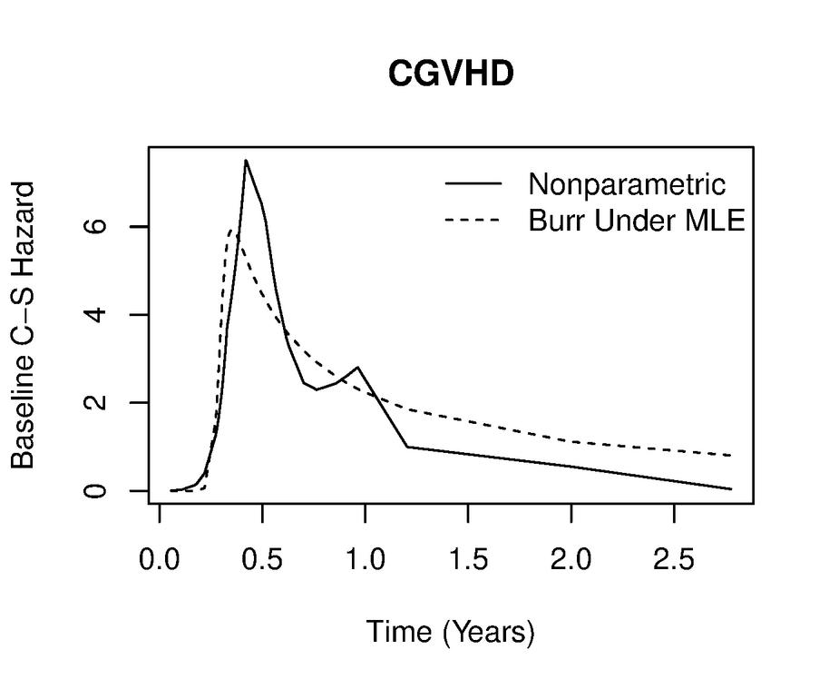
Figure 2 Cause specific hazard plotting for CGVHD event.

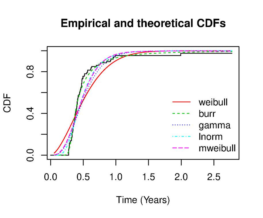
Figure 3 Fitted and empirical CDF’s for CGVHD event.

Table 5 Baseline parameters estimate and goodness of fit statistics for CGVHD event

Model	MLE	Loglikelihood	AIC	BIC
Burr Type XII	$\alpha$=16.25, $\lambda$ =0.137, a=0.299	37.5849	-69.1699	-61.3543
Weibull	Shape=1.66, Scale=0.596	-16.4583	36.9166	42.1269
Gamma	Shape=4.166, Rate=8.004	-1.3529	6.7058	11.9162
Lognormal	Meanlog=-0.781, Sdlog=0.44	13.6107	-23.2214	-18.0110
MWeibull	Shape 1=3.0714, Shape 2=-1.4954, Rate=14.3886	8.3458	-10.6918	-2.8762

Table 6 ML and Bayes estimates of the parameters with standard error for both causes

	CGVHD Cause					Other Cause
	${\alpha }_1$	${\lambda }_1$	$a_1$	${\beta }_{11}$	${\beta }_{12}$	${\alpha }_2$	${\lambda }_2$	$a_2$	${\beta }_{21}$	${\beta }_{22}$
MLE Estimate
Estimate	2.8726	1.0716	0.4127	-0.1075	-0.001	2.3882	0.0312	0.1551	2.5614*	-0.0423
S.E.	0.3164	0.6882	0.0443	0.2169	0.0123	1.1226	0.0273	0.0973	1.1051	0.0272
Bayes Estimates (Gamma Prior)
SELF	5.7435	0.5179	0.3564	0.1362	-0.0053	2.3718	0.0591	0.2039	-0.7559	-0.0459*
LLF $p=1.5$	5.3641	0.5084	0.356	0.1041	-0.0053	2.1171	0.056	0.1838	-0.9844	-0.0459*
LLF $p=-1.5$	6.2405	0.5282	0.3568	0.168	-0.0053	2.728	0.0633	0.2548	-0.5424	-0.0458*
SD	0.754	0.1148	0.0228	0.2064	0.0034	0.6317	0.0685	0.1943	0.5411	0.0084
Bayes Estimates (Weibull Prior)
SELF	6.531	0.4393	0.345	0.1292	-0.0052	2.6898	0.0389	0.1504	-0.7513	-0.046*
LLF $p=1.5$	6.0665	0.4327	0.3447	0.0976	-0.0052	2.2433	0.0382	0.1443	-0.9819	-0.0461*
LLF $p=-1.5$	7.0775	0.4464	0.3453	0.1611	-0.0052	3.4064	0.0397	0.1584	-0.5366	-0.046*
SD	0.8196	0.0953	0.0196	0.2058	0.0034	0.8666	0.0313	0.0954	0.5436	0.0084
Bayes Estimates (Lognormal Prior)
SELF	6.2882	0.4709	0.3493	0.1363	-0.0053	2.5324	0.0361	0.1381	-0.7502	-0.046*
LLF $p=1.5$	5.7157	0.462	0.349	0.1037	-0.0053	2.2727	0.0356	0.1332	-0.9761	-0.046*
LLF $p=-1.5$	7.2395	0.4807	0.3497	-0.169	0.0053	2.9708	0.0367	0.1442	0.543	0.0459*
SD	0.964	0.1117	0.0216	0.2087	0.0034	0.6567	0.0266	0.0849	0.5349	0.0085
*Significant effect
${\beta }_{j1}$ $=$ Regression Coefficient of treatments (BM, PB)
${\beta }_{j2}$ $=$ Regression Coefficient of age

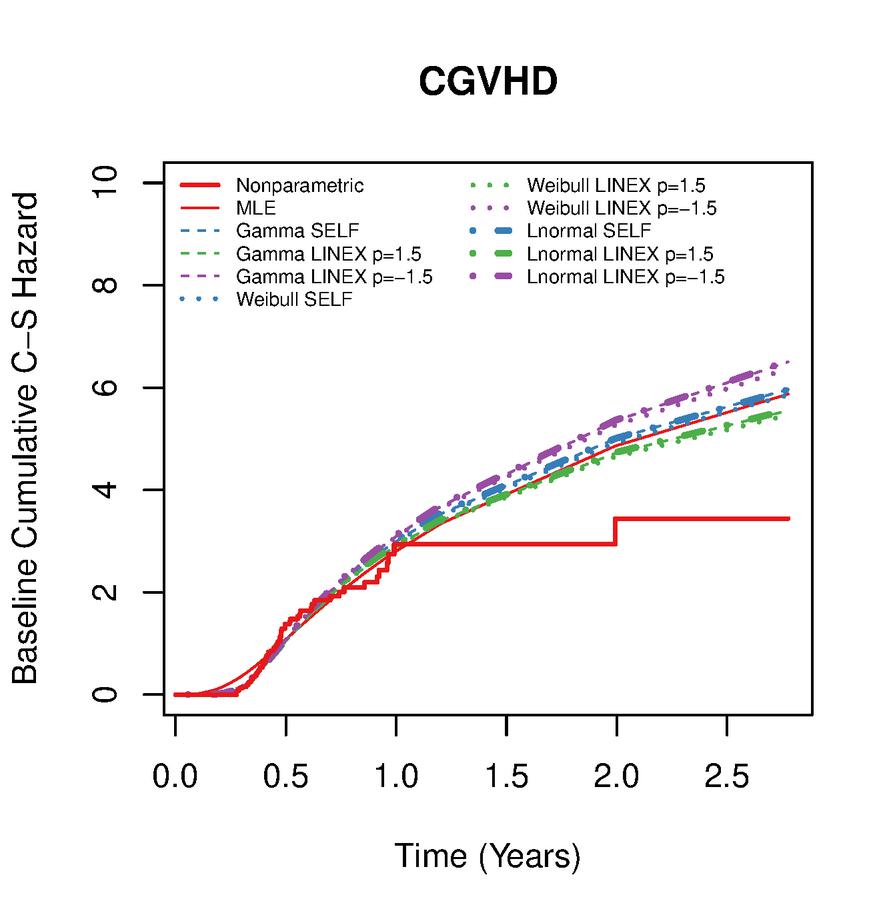
Figure 4 Baseline cumulative cause specific hazard for CGVHD event.

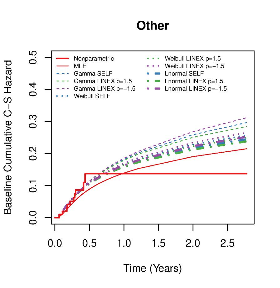
Figure 5 Baseline cumulative cause specific hazard for other event.

In order to illustrate our methodology, we used a subset of data of 100 patients with three types of endpoints: time to relapse, time to chronic graft versus host disease (CGVHD) and time to death (Pintilie, 2006). Survival for these patients was measured in years from the date of transplant to death of each specific event. For mathematically convenience we only use the two end points, one is CGVHD known as cause 1 and cause 2 is the combination of time to relapse and time to death. It is seen that out of 100 patients 86 patients experienced with CGVHD, and 10 patients experienced relapse and death, and 4 patients were right censored. The effect of two covariates such as treatments (BM, PB) and age is observed.

First, we characterize the shape of the cause specific hazard of CGVHD by nonparametrically and compared with proposed model. We found that shape of the cause specific hazard of CGVHD under both procedures are very close and it is initially increasing and then decreasing i.e. nonmonotone in nature (see, Figure 2). We therefore, compared the goodness of fit of the model with Weibull, gamma, modified Weibull distribution (MWeibull) (Lai et al., 2003) and lognormal distributions based on Akaike information criterion (AIC) and Bayesian information criterion (BIC). The fitting summary of the CGVHD are reported in Table 5. It is also observed that the AIC and BIC for CGVHD of Burr type XII distribution are least among the other distributions. The graphs of the empirical and fitted models are shown in Figure 3. Which shows that cumulative distribution function of Burr type XII distribution is very close to empirical other than the Weibull, gamma, modified Weibull and lognormal distributions.

Further, we also analyse the proposed model for competing events by applying both the estimation procedures. The estimates of baseline parameters and regression parameters with their standard error are given in Table 6. Figures 4 and 5 shows the estimated baseline cumulative cause specific hazard function for both the competing causes under proposed model and compared with nonparametric estimates. The nonparametric estimates are obtained without considering the situation of competing risks.

7 Conclusion

In this article, we consider the problem of competing risk estimation via cause specific hazard function using Burr type XII distribution as baseline model. The flexibility of the distribution has been demonstrated through the behaviour of probability density function and hazard function. It is also observed that it gives good fit for bone marrow transplant data. We utilized both classical and Bayes estimators under class of informative types of priors under SELF (symmetric) and LLF (asymmetric). Choice of lognormal and Weibull prior is satisfactory under SELF as well as LLF$(p=\pm 1.5).$ Appropriate convergence and identifiability of the model is observed in simulation study. In real data example, the estimates of cumulative cause specific hazard function for CGVHD cause and other causes very close to nonparametric estimates at the initial failure time points. It is observed that CGVHD has larger cumulative cause specific hazard compared to other causes. The treatments (BM, PB) and age have not any significant effect on CGVHD. But on other causes the effect of age is significant under Bayes estimates and treatments are significant under likelihood estimates.

References

Anjana, S., Sankaran, P.G., 2015. Parametric Analysis of Lifetime Data With Multiple Causes of Failure Using Cause Specific Reversed Hazard Rates. Calcutta Stat. Assoc. Bull. 67, 129–142.

Benichou, J., Gail, M.H., 1990. Estimates of absolute cause-specific risk in cohort studies. Biometrics 46, 813–826.

Beyersmann, J., Allignol, A., Schumacher, M., 2012. Competing risks and multistate models with R. Springer Science & Business Media. https://doi.org/10.1007/978-1-4614-2035-4

Bryant, J., Dignam, J.J., 2004. Semiparametric Models for Cumulative Incidence Functions. Biometrics 60, 182–190. https://doi.org/10.1111/j.0006-341X.2004.00149.x

Burr, I.W., 1942. Cumulative frequency functions. Ann. Math. Stat. 13, 215–232.

Byrnes, J.M., Lin, Y.J., Tsai, T.R., Lio, Y., 2019. Bayesian inference of $\delta$ = P(X $<$ Y) for Burr type XII distribution based on progressively first failure-censored samples. Mathematics 7, 794. https://doi.org/10.3390/math7090794

Couban, S., Simpson, D.R., Barnett, M.J., Bredeson, C., Hubesch, L., Howson-Jan, K., Shore, T.B., Walker, I.R., Browett, P., Messner, H.A., others, 2002. A randomized multicenter comparison of bone marrow and peripheral blood in recipients of matched sibling allogeneic transplants for myeloid malignancies. Blood, J. Am. Soc. Hematol. 100, 1525–1531.

Cox, D.R., 1972. Regression Models and Life-Tables. J. R. Stat. Soc. Ser. B 34, 187–220. https://doi.org/10.1111/j.2517-6161.1972.tb00899.x

Ge, M., Chen, M.H., 2012. Bayesian inference of the fully specified subdistribution model for survival data with competing risks. Lifetime Data Anal. 18, 339–363. https://doi.org/10.1007/s10985-012-9221-9

Geman, S., Geman, D., 1984. Stochastic relaxation, Gibbs distributions, and the Bayesian restoration of images. IEEE Trans. Pattern Anal. Mach. Intell. 6, 721–741.

Gupta, P.L., Gupta, R.C., Lvin, S.J., 1996. Analysis of failure time data by burr distribution. Commun. Stat. Methods 25, 2013–2024.

Hastings, W.K., 1970. Monte Carlo sampling methods using Markov chains and their applications. Biometrika 57, 97–109.

Jeong, J.H., Fine, J., 2006. Direct parametric inference for the cumulative incidence function. J. R. Stat. Soc. Ser. C Appl. Stat. 55, 187–200. https://doi.org/10.1111/j.1467-9876.2006.00532.x

Kalbfleisch, J.D., Prentice, R.L., 2002. The Statistical Analysis of Failure Time Data. John Wiley & Sons. https://doi.org/10.1002/9781118032985

Kehinde, O., Osebi, A., Ganiyu, D., 2018. A New Class of Generalized Burr III Distribution for Lifetime Data. Int. J. Stat. Distrib. Appl. 4, 6–21.

Lai, C.D., Xie, M., Murthy, D.N.P., 2003. A modified Weibull distribution. Reliab. IEEE Trans. 52, 33–37. https://doi.org/10.1109/TR.2002.805788

Lawless, J.F., 2014. Parametric Models in Survival Analysis. Encycl. Biostat. https://doi.org/10.1002/0470011815.b2a11056

Lee, M., 2019. Parametric inference for quantile event times with adjustment for covariates on competing risks data. J. Appl. Stat. 46, 2128–2144. https://doi.org/10.1080/02664763.2019.1577370

Lunn, D., Jackson, C., Best, N., Spiegelhalter, D., Thomas, A., 2012. The BUGS book: A practical introduction to Bayesian analysis. Chapman and Hall/CRC.

Okasha, H.M., Shrahili, M., 2017. A New Extended Burr XII Distribution with Applications. J. Comput. Theor. Nanosci. 14, 5261–5269.

Pintilie, M., 2006. Competing risks: a practical perspective. John Wiley & Sons.

Prentice, R.L., Kalbfleisch, J.D., Peterson, A. V, Flournoy, N., Farewell, V.T., Breslow, N.E., 1978. The analysis of failure times in the presence of competing risks. Biometrics 34, 541–54.

Robert, C.P., Casella, G., Casella, G., 2010. Introducing monte carlo methods with r. Springer.

Sen, A., Banerjee, M., Li, Y., Noone, A.-M.M., 2010. A Bayesian approach to competing risks analysis with masked cause of death. Stat. Med. 29, 1681–1695. https://doi.org/10.1002/sim.3894

Sinha, S.K., 1998. Bayesian Estimation. New Age International (P) Limited Publisher.

Soliman, A.A., Abd Ellah, A.H., Sultan, K.S., 2006. Comparison of estimates using record statistics from Weibull model: Bayesian and non-Bayesian approaches. Comput. Stat. Data Anal. 51, 2065–2077.

Soliman, A.A., Ellah, A.H.A., Abou-Elheggag, N.A., Modhesh, A.A., 2011. Bayesian Inference and Prediction of Burr Type XII Distribution for Progressive First Failure Censored Sampling. Intell. Inf. Manag. 03, 175–185. https://doi.org/10.4236/iim.2011.35021

Sreedevi, E.P., Sankaran, P.G., 2012. A semiparametric bayesian approach for the analysis of competing risks data. Commun. Stat. - Theory Methods 41, 2803–2818. https://doi.org/10.1080/03610920903551781

Biographies

H. Rehman was born in 1993. He is a Ph.D. student in the Department of statistics, Pondicherry University, India, since August, 2017. He attended the Aligarh Muslim University, Aligarh, India where he received his B.Sc. (Hons.) in Statistics in 2014 and M.Sc. in Statistics in 2016. His research interests include survival analysis and its application, competing risks models, Bayesian estimation, and statistical computing.

N. Chandra serving as permanent faculty member in Department of Statistics, Ramanujan School of Mathematical Sciences at Pondicherry University, Pondicherry, India. He received Ph.D. Statistics from Banaras Hindu University, India and recipient of Senior Research Fellowship under major research project(MRP) sponsored by Department of Science and Technology, MHRD, Government of India. He supervised number of students for M.Sc. dissertation and research students for Ph.D. thesis in Statistics disciplines. He has completed MRP sponsored by University Grants Commission, India. His research interests includes Bayesian Inference, Reliability Theory (Estimation in accelerated life testing, Stress-Strength Models, Augmenting strength Models, bivariate models in reliability) and Survival Analysis (New life time distributions, characterizations and application, Estimation in Competing risks modelling, survival modelling of time to events in medical data).

Fatemeh Sadat Hosseini-Baharanchi received her B.Sc. degree in Statistics and M.Sc. degree in Biostatistics from Tehran University of Medical Sciences; and Ph.D. degree in Biostatistics in 2016 from Tarbiat Modares University, Iran. Fatemeh was a visiting scholar in University of Connecticut, USA 2015. She is working in Iran University of Medical Sciences, Iran as an assistant professor in Biostatistics department since 2016. She is experienced in statistical modeling especially survival modeling and joint modeling of survival data and longitudinal measurements, especially in medical area. In addition, Fatemeh, as a member of international federation of Inventors Association, Geneva, Switzerland, helps students to pass the process of idea-to-patent as well as inventors to protect their intellectual property. She’s been focused on personal development, personal branding and innovative business models generation since 2018.

Ahmad Reza Baghestani received his B.Sc. degree in Statistics from Shahid Beheshti University and M.Sc. degree in Statistics from Tehran University of Medical Sciences; and Ph.D. degree in Biostatistics in 2010 from Tarbiat Modares University, Iran. He is associate professor in Biostatistics department in Shahid Beheshti University of Medical Sciences, Iran since 2011. He is fully-experienced in survival modeling, joint modeling, defective distributions, and competing risks analysis.

Journal of Reliability and Statistical Studies, Vol. 13_2-4, 325–348.
doi: 10.13052/jrss0974-8024.13246
© 2020 River Publishers

Abstract

1 Introduction

2 Model Formulation of Cause Specific Hazard Function

3 Maximum Likelihood (ML) Estimation

4 Bayesian Method of Estimation

5 Simulation Study

6 Real Life Application

7 Conclusion

References

Biographies