Availability Analysis of Hybrid Systems Consisting of Main Units and Cold Standby Processors

Ibrahim Yusuf^{1, *}, Nafisatu Muhammad Usman² and Saminu Iliyasu Bala¹

¹Department of Mathematical Sciences, Bayero University, Kano, Nigeria

²Department of Arts and Humanity, School of General Studies, Kano State Polytechnic, Kano, Nigeria

E-mail: iyusuf.mth@buk.edu.ng; mamankhairat2015@gmail.com; sibala.mth@buk.edu.ng

^*Corresponding Author

Received 01 September 2020; Accepted 08 December 2020; Publication 05 January 2021

Abstract

The present paper studies availability of four hybrid systems configured as series-parallel systems. Each system or configuration consisting of main units and their corresponding processors. Configuration I consist of three processors is a 2-out-of-3 unit connected to 2-out-of-3 processors, Configuration II is a 2-out-of-3 unit connected to 2-out-of-4 processors, Configuration III is a 2-out-of-4 unit connected to 2-out-of-4 processors while Configuration IV is a 2-out-of-4 unit connected to 2-out-of-3 processors. The failure and repair times of units and their processors are assumed to be exponentially distributed. Explicit expressions for steady state availability are developed for each system using first order linear differential difference equations and validated by performing numerical experiments. Analysis of the effect of various system parameters on availability was performed. Graphical illustrations are given to highlight important results. The systems are ranked based on their availability and found that Configuration IV is better. Sensitivity analysis on the model’s outcomes are performed using partial rank correlation coefficients (PRCC) to determine the most critical parameters leading to increase (decrease) in the value of availability.

Keywords: Availability, processor, configuration, main unit, series parallel.

1 Introduction

Many engineering, industrial or manufacturing systems are hybrid in nature, consisting of components, units or subsystems arrange as parallel, series, series-parallel, parallel-series or k-out-of-n system. These manufacturing, industrial and engineering systems are hybrid in nature consisting of build-in similar and dissimilar units, external unit, etc. Such system can only work with the help of external processors/units/devices linked to the system. Examples of such systems can be found in computer systems, power plants, manufacturing systems and industrial systems such as feeding, crushing, refining, steam generation, evaporation, crystallization, fertilizer plant, crystallization unit of a sugar plant, piston manufacturing plant, etc. Failure of the entire units or external processors/units/devices leads to the failure of the system called complete failure and the system operation must ceased whereas the failure of a unit or a external processors/units/devices with standby in the configuration is called partial failure. Due to their importance in production output, customer’s satisfaction as well as revenue mobilisation, reliability and availability analysis of such systems is of paramount important. Reliability and availability of systems are improved through redundancy. There are different forms of redundancy used in improving the system reliability leading to system safety, quality of the product, adequate production output, less maintenance cost, high revenue mobilisation, customer’s satisfaction, etc. Such forms of redundancy can be cold, hot, warm or k-out-of-n system.

One of the forms of redundancy is the 2-out-of-3 system which has wide application in industrial setting. Moreover, the k-out-of-n works if and only if at least k of the n components works. Example of the 2-out-of-3 system can be seen in a communication system with three transmitters and the average message load may be such that at least two transmitters must be operational at all times or critical messages may be lost. Thus, the transmission subsystem functions as a 2-out-of-3: G system. Due to their importance in industries and design, the 2-out-of-3 systems have received attention from different researchers. Bhardwaj and Chander [2] propose method of analysing reliability and cost benefit analysis of 2-out-of-3 redundant system with general distribution of repair and waiting time. Bhardwaj and Malik [3] studied MTSF and cost effectiveness of 2-out-of-3 standby system with probability of repair and inspection. Chander and Bhardwaj [4] discussed the reliability and economic analysis of 2-out-of-3 redundant system with priority to repair. Chander and Bhardwaj [5] discussed the reliability and economic analysis of 2-out-of-3 redundant system with priority and replacement. Chander and Bhardwaj [6] analyzed reliability modelling and analysis of 2-out-of-3 redundant system subject to conditional arrival time of server. Khatab et al. [11] analyzed the availability of of k-out-of-n: G systems with non-identical components subject to repair priorities. Li et al. [13] presented reliability analysis of a repairable k-out-of-n system with some components being suspended when the system is down. Yusuf and Hussaini [16] deal with evaluation of reliability and availability characteristics of 2-out-3 standby system under a perfect repair condition.

Many researchers have presented their works in the field of reliability and availability analysis of engineering, industrial and manufacturing system by evaluating the reliability characteristics of the systems under the different types of failure, preventive maintenance, repairs and replacement actions. To cite few, Aliyu et al. [1] discussed the availability and profit optimization of series-parallel system with linear consecutive cold standby unit. Garg [7] proposed methods of PSO and fuzzy to analyzed the reliability, availability and maintainability analysis of industrial systems. Garg [8] discussed an approach for analyzing the reliability of series-parallel system using credibility theory and different types of intuitionistic fuzzy numbers. Garg [9] presented an approach for analyzing the reliability of industrial system using fuzzy kolmogrov’s differential equations. Niwas and Garg [14] dealt with an approach for analyzing the reliability and profit of an industrial system based on the cost-free warranty policy. Garg [10] focus on the performance of an industrial system using soft computing based hybridized technique Kumar et al. [12] dealt with assessment of reliability of a system by applying hesitant fuzzy set. Singh and Rawal [15] presented study on availability, MTTF, and cost analysis of the complex system under preemptive resume repair policy using copula distribution. Yusuf et al. [17] discussed the reliability Analysis of a linear consecutive 2-out-of-3 System in the presence of supporting device and repairable service station. Yusuf [18] dealt with reliability modeling of a parallel system with a supporting device and two types of preventive maintenance.

Although literature above and the existing ones have carried out on reliability analysis for engineering, industrial and manufacturing systems. Little is known on reliability and availability of such system working with the aid of an external processor supporting the working of the entire system. The present paper tends to develop an availability models of different configuration connected to external processor for operation to addresses the gap. The present paper studies availability of four hybrid systems configured as series-parallel systems in which each system or configuration consisting of main units and their corresponding processors. The systems or configurations have been studied by using the first order linear differential difference equations to derive the corresponding availability models for each configuration. Comparative analysis of the study among configurations been carried out to determine the optimal configuration. Surface plots and partial rank correlation have also been computed in the study. The organization of the paper is as follows. Section 2 contains a description of the configurations under study. Section 3 presents formulations of the models. The results of our numerical simulations are presented and discussed in Section 4. Finally, we make some concluding remarks in Section 5.

2 Description of the Configurations

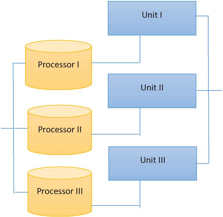
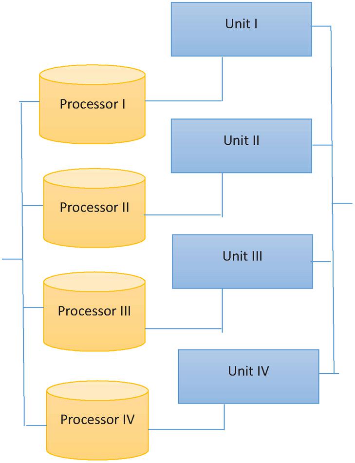
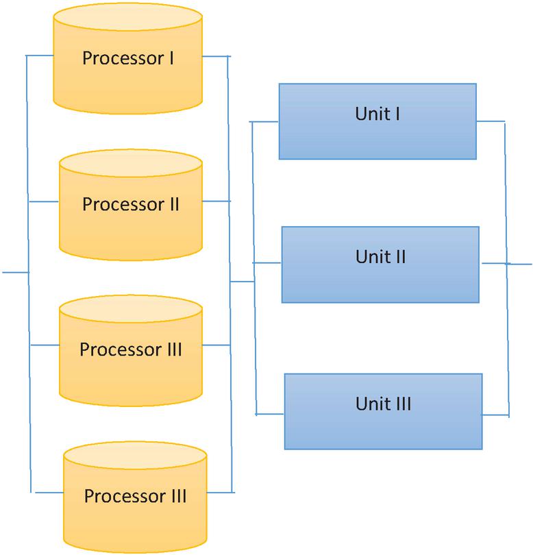
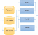
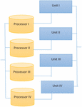
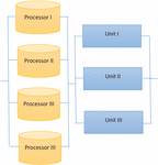
Figure 1 depict Configuration I consisting of three processors is a 2-out-of-3 unit connected to 2-out-of-3 processors, Figure 2 displayed Configuration II having 2-out-of-3 unit connected to 2-out-of-4 processors, Figure 3 depict Configuration III consisting of 2-out-of-4 unit connected to 2-out-of-4 processors while Figure 4 is Configuration IV consisting of 2-out-of-4 unit connected to 2-out-of-3 processors. Each configuration composed of two subsystems. Subsystem I of each configuration consist of the identical cold standby processors. Subsystem II each configuration consists of identical cold standby main units. The processors in each subsystem received the signal, process it and forward to the main unit for usage. Each of the main unit and processor fails with exponential failure distribution with parameter ${\beta }_1$ and ${\beta }_2$, exponential repair distribution with parameter ${\alpha }_1$ and ${\alpha }_2$ respectively. When one of the main unit (processor) failed, which occurs with failure rate ${\beta }_1({\beta }_2)$, it is repaired with the rate ${\alpha }_1({\alpha }_2)$ and the corresponding standby main unit (processor) then carries out the function of the failed main unit (processor). It is assumed that switching from standby to operation is perfect. System failure results from the failure of subsystem I or subsystem II or both.

Figure 1 Reliability block diagram of configuration I.

Figure 2 Reliability block diagram of configuration II.

Figure 3 Reliability block diagram of configuration III.

Figure 4 Reliability block diagram of configuration IV.

3 Availability Models Formulation

3.1 Availability Formulation of Configuration I

Define $p_i(t)$ to be the probability that the system is in state $i$ at time$t$. Thus, $p_0(t)$, $p_1(t)$, $p_2(t)$, $p_3(t)$, $p_4(t)$, $p_5(t)$and $p_6(t)$ are probabilities that the system is in state $S_0$, $S_1$, $S_2$,$S_3$, $S_4$, $S_5$ and $S_6$. Let$P(t)=[p_1(t),p_2(t),\mathrm{\dots },p_{11}(t)]$ be the probability row vector with initial conditions

$$p_k(0)=\{\begin{array}{cc}1,\hfill & k=0\hfill \\ 0,\hfill & k=1,2,3,4,5,6\hfill \end{array}$$

The corresponding set of differential-difference-equations for configuration I are

$$\begin{array}{c}\frac{d{p}_0(t)}{dt}=-\left(2{\beta }_1+2{\beta }_2\right)p_0(t)+{\alpha }_1{p}_1(t)+{\alpha }_2{p}_2(t)\hfill \\ \frac{d{p}_1(t)}{dt}=-\left(2{\beta }_1+2{\beta }_2+{\alpha }_1\right)p_1(t)+2{\beta }_1{p}_0(t)+{\alpha }_1{p}_3(t)+{\alpha }_2{p}_5(t)\hfill \\ \frac{d{p}_2(t)}{dt}=-\left(2{\beta }_1+2{\beta }_2+{\alpha }_2\right)p_2(t)+2{\beta }_2{p}_0(t)+{\alpha }_2{p}_4(t)+{\alpha }_1{p}_6(t)\hfill \\ \frac{d{p}_3(t)}{dt}=-{\alpha }_1{p}_3(t)+2{\beta }_1{p}_1(t)\hfill \\ \frac{d{p}_4(t)}{dt}=-{\alpha }_2{p}_4(t)+2{\beta }_2{p}_4(t)\hfill \\ \frac{d{p}_5(t)}{dt}=-{\alpha }_2{p}_5(t)+2{\beta }_2{p}_1(t)\hfill \\ \frac{d{p}_6(t)}{dt}=-{\alpha }_1{p}_6(t)+2{\beta }_1{p}_2(t)\hfill \end{array}\}$$

(1)

To compute the availability of configuration I, the differential difference equation given in (1) are expressed in the matrix format

$\left(\begin{array}{c}\hfill p_0^{\prime }\hfill \\ \hfill p_1^{\prime }\hfill \\ \hfill p_2^{\prime }\hfill \\ \hfill p_3^{\prime }\hfill \\ \hfill p_4^{\prime }\hfill \\ \hfill p_5^{\prime }\hfill \\ \hfill p_6^{\prime }\hfill \end{array}\right)$

$=\left(\begin{array}{ccccccc}\hfill -(2{\beta }_1+2{\beta }_2)\hfill & \hfill {\alpha }_1\hfill & \hfill {\alpha }_2\hfill & \hfill 0\hfill & \hfill 0\hfill & \hfill 0\hfill & \hfill 0\hfill \\ \hfill 2{\beta }_1\hfill & \hfill -(2{\beta }_1\hfill & \hfill 0\hfill & \hfill {\alpha }_1\hfill & \hfill 0\hfill & \hfill {\alpha }_2\hfill & \hfill 0\hfill \\ & \hfill +2{\beta }_2\hfill & & & & & \\ & \hfill +{\alpha }_1)\hfill & & & & & \\ \hfill 2{\beta }_2\hfill & \hfill 0\hfill & \hfill -(2{\beta }_1\hfill & \hfill 0\hfill & \hfill {\alpha }_2\hfill & \hfill 0\hfill & \hfill {\alpha }_1\hfill \\ & & \hfill +2{\beta }_2\hfill & & & & \\ & & \hfill +{\alpha }_2)\hfill & & & & \\ \hfill 0\hfill & \hfill 2{\beta }_1\hfill & \hfill 0\hfill & \hfill -{\alpha }_1\hfill & \hfill 0\hfill & \hfill 0\hfill & \hfill 0\hfill \\ \hfill 0\hfill & \hfill 0\hfill & \hfill 2{\beta }_2\hfill & \hfill 0\hfill & \hfill -{\alpha }_2\hfill & \hfill 0\hfill & \hfill 0\hfill \\ \hfill 0\hfill & \hfill 2\beta 2\hfill & \hfill 0\hfill & \hfill 0\hfill & \hfill 0\hfill & \hfill -{\alpha }_2\hfill & \hfill 0\hfill \\ \hfill 0\hfill & \hfill 0\hfill & \hfill 2{\beta }_1\hfill & \hfill 0\hfill & \hfill 0\hfill & \hfill 0\hfill & \hfill -{\alpha }_1\hfill \end{array}\right)\left(\begin{array}{c}\hfill p_0(t)\hfill \\ \hfill p_1(t)\hfill \\ \hfill p_2(t)\hfill \\ \hfill p_3(t)\hfill \\ \hfill p_4(t)\hfill \\ \hfill p_5(t)\hfill \\ \hfill p_6(t)\hfill \end{array}\right)$

(2)

Setting left side of (2) to zero in steady state to give:

$\left(\begin{array}{ccccccc}\hfill -(2{\beta }_1\hfill & \hfill {\alpha }_1\hfill & \hfill {\alpha }_2\hfill & \hfill 0\hfill & \hfill 0\hfill & \hfill 0\hfill & \hfill 0\hfill \\ \hfill +2{\beta }_2)\hfill & & & & & & \\ \hfill 2{\beta }_1\hfill & \hfill -(2{\beta }_1\hfill & \hfill 0\hfill & \hfill {\alpha }_1\hfill & \hfill 0\hfill & \hfill {\alpha }_2\hfill & \hfill 0\hfill \\ & \hfill +2{\beta }_2\hfill & & & & & \\ & \hfill +{\alpha }_1)\hfill & & & & & \\ \hfill 2{\beta }_2\hfill & \hfill 0\hfill & \hfill -(2{\beta }_1\hfill & \hfill 0\hfill & \hfill {\alpha }_2\hfill & \hfill 0\hfill & \hfill {\alpha }_1\hfill \\ & & \hfill +2{\beta }_2\hfill & & & & \\ & & \hfill +{\alpha }_2)\hfill & & & & \\ \hfill 0\hfill & \hfill 2{\beta }_1\hfill & \hfill 0\hfill & \hfill -{\alpha }_1\hfill & \hfill 0\hfill & \hfill 0\hfill & \hfill 0\hfill \\ \hfill 0\hfill & \hfill 0\hfill & \hfill 2{\beta }_2\hfill & \hfill 0\hfill & \hfill -{\alpha }_2\hfill & \hfill 0\hfill & \hfill 0\hfill \\ \hfill 0\hfill & \hfill 2{\beta }_2\hfill & \hfill 0\hfill & \hfill 0\hfill & \hfill 0\hfill & \hfill -{\alpha }_2\hfill & \hfill 0\hfill \\ \hfill 0\hfill & \hfill 0\hfill & \hfill 2{\beta }_1\hfill & \hfill 0\hfill & \hfill 0\hfill & \hfill 0\hfill & \hfill -{\alpha }_1\hfill \end{array}\right)\left(\begin{array}{c}\hfill p_0(t)\hfill \\ \hfill p_1(t)\hfill \\ \hfill p_2(t)\hfill \\ \hfill p_3(t)\hfill \\ \hfill p_4(t)\hfill \\ \hfill p_5(t)\hfill \\ \hfill p_6(t)\hfill \end{array}\right)=\left(\begin{array}{c}\hfill 0\hfill \\ \hfill 0\hfill \\ \hfill 0\hfill \\ \hfill 0\hfill \\ \hfill 0\hfill \\ \hfill 0\hfill \\ \hfill 0\hfill \end{array}\right)$

(3)

Combining (3) and normalizing condition

$$\sum _{n=0}^6{p}_n(\mathrm{\infty })=1$$

(4)

to give

$\left(\begin{array}{ccccccc}\hfill -(2{\beta }_1\hfill & \hfill {\alpha }_1\hfill & \hfill {\alpha }_2\hfill & \hfill 0\hfill & \hfill 0\hfill & \hfill 0\hfill & \hfill 0\hfill \\ \hfill +2{\beta }_2)\hfill & & & & & & \\ \hfill 2{\beta }_1\hfill & \hfill -(2{\beta }_1\hfill & \hfill 0\hfill & \hfill {\alpha }_1\hfill & \hfill 0\hfill & \hfill {\alpha }_2\hfill & \hfill 0\hfill \\ & \hfill +2{\beta }_2\hfill & & & & & \\ & \hfill +{\alpha }_1)\hfill & & & & & \\ \hfill 2{\beta }_2\hfill & \hfill 0\hfill & \hfill -(2{\beta }_1\hfill & \hfill 0\hfill & \hfill {\alpha }_2\hfill & \hfill 0\hfill & \hfill {\alpha }_1\hfill \\ & & \hfill +2{\beta }_2\hfill & & & & \\ & & \hfill +{\alpha }_2)\hfill & & & & \\ \hfill 0\hfill & \hfill 2{\beta }_1\hfill & \hfill 0\hfill & \hfill -{\alpha }_1\hfill & \hfill 0\hfill & \hfill 0\hfill & \hfill 0\hfill \\ \hfill 0\hfill & \hfill 0\hfill & \hfill 2{\beta }_2\hfill & \hfill 0\hfill & \hfill -{\alpha }_2\hfill & \hfill 0\hfill & \hfill 0\hfill \\ \hfill 0\hfill & \hfill 2{\beta }_2\hfill & \hfill 0\hfill & \hfill 0\hfill & \hfill 0\hfill & \hfill -{\alpha }_2\hfill & \hfill 0\hfill \\ \hfill 1\hfill & \hfill 1\hfill & \hfill 1\hfill & \hfill 1\hfill & \hfill 1\hfill & \hfill 1\hfill & \hfill 1\hfill \end{array}\right)\left(\begin{array}{c}\hfill p_0(t)\hfill \\ \hfill p_1(t)\hfill \\ \hfill p_2(t)\hfill \\ \hfill p_3(t)\hfill \\ \hfill p_4(t)\hfill \\ \hfill p_5(t)\hfill \\ \hfill p_6(t)\hfill \end{array}\right)=\left(\begin{array}{c}\hfill 0\hfill \\ \hfill 0\hfill \\ \hfill 0\hfill \\ \hfill 0\hfill \\ \hfill 0\hfill \\ \hfill 0\hfill \\ \hfill 1\hfill \end{array}\right)$

(5)

To obtain the states probabilities $p_k(t)$, (5) is solved using MATLAB package.

The steady-state availability for Configuration I is given by

$A_{V1}(\mathrm{\infty })$	$=p_0(\mathrm{\infty })+p_1(\mathrm{\infty })+p_2(\mathrm{\infty })$
	$={\displaystyle \frac{{\alpha }_1^2{\alpha }_2^2+2{\alpha }_1{\alpha }_2^2{\beta }_1+2{\alpha }_1^2{\alpha }_2{\beta }_2}{4{\alpha }_2^2{\beta }_1^2+2{\alpha }_1{\alpha }_2^2{\beta }_1+2{\alpha }_1^2{\alpha }_2{\beta }_2+{\alpha }_1^2{\alpha }_2^2+8{\alpha }_1{\alpha }_2{\beta }_1{\beta }_2+4{\alpha }_1^2{\beta }_2^2}}$	(6)

3.2 Availability Formulation of Configuration II

To compute the availability of configuration II, the differential difference equation is expressed in the form

$\left(\begin{array}{c}\hfill p_0^{\prime }\hfill \\ \hfill p_1^{\prime }\hfill \\ \hfill p_2^{\prime }\hfill \\ \hfill p_3^{\prime }\hfill \\ \hfill p_4^{\prime }\hfill \\ \hfill p_5^{\prime }\hfill \\ \hfill p_6^{\prime }\hfill \\ \hfill p_7^{\prime }\hfill \\ \hfill p_8^{\prime }\hfill \\ \hfill p_9^{\prime }\hfill \\ \hfill p_{10}^{\prime }\hfill \end{array}\right)$
$\mathrm{\hspace{1em}\hspace{1em}}=\left(\begin{array}{ccccccccccc}\hfill -h_1\hfill & \hfill {\alpha }_1\hfill & \hfill {\alpha }_2\hfill & \hfill 0\hfill & \hfill 0\hfill & \hfill 0\hfill & \hfill 0\hfill & \hfill 0\hfill & \hfill 0\hfill & \hfill 0\hfill & \hfill 0\hfill \\ \hfill 2{\beta }_1\hfill & \hfill -h_2\hfill & \hfill 0\hfill & \hfill {\alpha }_1\hfill & \hfill 0\hfill & \hfill 0\hfill & \hfill {\alpha }_2\hfill & \hfill 0\hfill & \hfill 0\hfill & \hfill 0\hfill & \hfill 0\hfill \\ \hfill 2{\beta }_2\hfill & \hfill 0\hfill & \hfill -h_3\hfill & \hfill 0\hfill & \hfill {\alpha }_2\hfill & \hfill 0\hfill & \hfill {\alpha }_1\hfill & \hfill 0\hfill & \hfill 0\hfill & \hfill 0\hfill & \hfill 0\hfill \\ \hfill 0\hfill & \hfill 2{\beta }_1\hfill & \hfill 0\hfill & \hfill -{\alpha }_1\hfill & \hfill 0\hfill & \hfill 0\hfill & \hfill 0\hfill & \hfill 0\hfill & \hfill 0\hfill & \hfill 0\hfill & \hfill 0\hfill \\ \hfill 0\hfill & \hfill 0\hfill & \hfill 2{\beta }_2\hfill & \hfill 0\hfill & \hfill -h_2\hfill & \hfill {\alpha }_2\hfill & \hfill 0\hfill & \hfill 0\hfill & \hfill {\alpha }_1\hfill & \hfill 0\hfill & \hfill 0\hfill \\ \hfill 0\hfill & \hfill 0\hfill & \hfill 0\hfill & \hfill 0\hfill & \hfill 2{\beta }_2\hfill & \hfill -{\alpha }_2\hfill & \hfill 0\hfill & \hfill 0\hfill & \hfill 0\hfill & \hfill 0\hfill & \hfill 0\hfill \\ \hfill 0\hfill & \hfill 2{\beta }_2\hfill & \hfill 2{\beta }_1\hfill & \hfill 0\hfill & \hfill 0\hfill & \hfill 0\hfill & \hfill -h_4\hfill & \hfill {\alpha }_1\hfill & \hfill {\alpha }_2\hfill & \hfill 0\hfill & \hfill 0\hfill \\ \hfill 0\hfill & \hfill 0\hfill & \hfill 0\hfill & \hfill 0\hfill & \hfill 0\hfill & \hfill 0\hfill & \hfill 2{\beta }_1\hfill & \hfill -{\alpha }_1\hfill & \hfill 0\hfill & \hfill 0\hfill & \hfill 0\hfill \\ \hfill 0\hfill & \hfill 0\hfill & \hfill 0\hfill & \hfill 0\hfill & \hfill 2{\beta }_1\hfill & \hfill 0\hfill & \hfill 2{\beta }_2\hfill & \hfill 0\hfill & \hfill -h_4\hfill & \hfill {\alpha }_1\hfill & \hfill {\alpha }_2\hfill \\ \hfill 0\hfill & \hfill 0\hfill & \hfill 0\hfill & \hfill 0\hfill & \hfill 0\hfill & \hfill 0\hfill & \hfill 0\hfill & \hfill 0\hfill & \hfill 2{\beta }_1\hfill & \hfill -{\alpha }_1\hfill & \hfill 0\hfill \\ \hfill 0\hfill & \hfill 0\hfill & \hfill 0\hfill & \hfill 0\hfill & \hfill 0\hfill & \hfill 0\hfill & \hfill 0\hfill & \hfill 0\hfill & \hfill 2{\beta }_2\hfill & \hfill 0\hfill & \hfill -{\alpha }_2\hfill \end{array}\right)$
$\mathrm{\hspace{1em}\hspace{1em}}\left(\begin{array}{c}\hfill p_0(\mathrm{\infty })\hfill \\ \hfill p_1(\mathrm{\infty })\hfill \\ \hfill p_2(\mathrm{\infty })\hfill \\ \hfill p_3(\mathrm{\infty })\hfill \\ \hfill p_4(\mathrm{\infty })\hfill \\ \hfill p_5(\mathrm{\infty })\hfill \\ \hfill p_6(\mathrm{\infty })\hfill \\ \hfill p_7(\mathrm{\infty })\hfill \\ \hfill p_8(\mathrm{\infty })\hfill \\ \hfill p_9(\mathrm{\infty })\hfill \\ \hfill p_{10}(\mathrm{\infty })\hfill \end{array}\right)$	(7)

Where $h_1=(2{\beta }_1+2{\beta }_2)$, $h_2=(2{\beta }_1+2{\beta }_2+{\alpha }_1)$, $h_3=(2{\beta }_1+2{\beta }_2+{\alpha }_2)$, $h_4=(2\beta {}_1+2{\beta }_2+{\alpha }_1+{\alpha }_2)$.

From similar procedure described above, left hand side of (7) is set to zero in steady state and becomes

$\left(\begin{array}{ccccccccccc}\hfill -h_1\hfill & \hfill {\alpha }_1\hfill & \hfill {\alpha }_2\hfill & \hfill 0\hfill & \hfill 0\hfill & \hfill 0\hfill & \hfill 0\hfill & \hfill 0\hfill & \hfill 0\hfill & \hfill 0\hfill & \hfill 0\hfill \\ \hfill 2{\beta }_1\hfill & \hfill -h_2\hfill & \hfill 0\hfill & \hfill {\alpha }_1\hfill & \hfill 0\hfill & \hfill 0\hfill & \hfill {\alpha }_2\hfill & \hfill 0\hfill & \hfill 0\hfill & \hfill 0\hfill & \hfill 0\hfill \\ \hfill 2{\beta }_2\hfill & \hfill 0\hfill & \hfill -h_3\hfill & \hfill 0\hfill & \hfill {\alpha }_2\hfill & \hfill 0\hfill & \hfill {\alpha }_1\hfill & \hfill 0\hfill & \hfill 0\hfill & \hfill 0\hfill & \hfill 0\hfill \\ \hfill 0\hfill & \hfill 2{\beta }_1\hfill & \hfill 0\hfill & \hfill -{\alpha }_1\hfill & \hfill 0\hfill & \hfill 0\hfill & \hfill 0\hfill & \hfill 0\hfill & \hfill 0\hfill & \hfill 0\hfill & \hfill 0\hfill \\ \hfill 0\hfill & \hfill 0\hfill & \hfill 2{\beta }_2\hfill & \hfill 0\hfill & \hfill -h_2\hfill & \hfill {\alpha }_2\hfill & \hfill 0\hfill & \hfill 0\hfill & \hfill {\alpha }_1\hfill & \hfill 0\hfill & \hfill 0\hfill \\ \hfill 0\hfill & \hfill 0\hfill & \hfill 0\hfill & \hfill 0\hfill & \hfill 2{\beta }_2\hfill & \hfill -{\alpha }_2\hfill & \hfill 0\hfill & \hfill 0\hfill & \hfill 0\hfill & \hfill 0\hfill & \hfill 0\hfill \\ \hfill 0\hfill & \hfill 2{\beta }_2\hfill & \hfill 2{\beta }_1\hfill & \hfill 0\hfill & \hfill 0\hfill & \hfill 0\hfill & \hfill -h_4\hfill & \hfill {\alpha }_1\hfill & \hfill {\alpha }_2\hfill & \hfill 0\hfill & \hfill 0\hfill \\ \hfill 0\hfill & \hfill 0\hfill & \hfill 0\hfill & \hfill 0\hfill & \hfill 0\hfill & \hfill 0\hfill & \hfill 2{\beta }_1\hfill & \hfill -{\alpha }_1\hfill & \hfill 0\hfill & \hfill 0\hfill & \hfill 0\hfill \\ \hfill 0\hfill & \hfill 0\hfill & \hfill 0\hfill & \hfill 0\hfill & \hfill 2{\beta }_1\hfill & \hfill 0\hfill & \hfill 2{\beta }_2\hfill & \hfill 0\hfill & \hfill -h_4\hfill & \hfill {\alpha }_1\hfill & \hfill {\alpha }_2\hfill \\ \hfill 0\hfill & \hfill 0\hfill & \hfill 0\hfill & \hfill 0\hfill & \hfill 0\hfill & \hfill 0\hfill & \hfill 0\hfill & \hfill 0\hfill & \hfill 2{\beta }_1\hfill & \hfill -{\alpha }_1\hfill & \hfill 0\hfill \\ \hfill 0\hfill & \hfill 0\hfill & \hfill 0\hfill & \hfill 0\hfill & \hfill 0\hfill & \hfill 0\hfill & \hfill 0\hfill & \hfill 0\hfill & \hfill 2{\beta }_2\hfill & \hfill 0\hfill & \hfill -{\alpha }_2\hfill \end{array}\right)$

$\mathrm{\hspace{1em}\hspace{1em}}\left(\begin{array}{c}\hfill p_0(\mathrm{\infty })\hfill \\ \hfill p_1(\mathrm{\infty })\hfill \\ \hfill p_2(\mathrm{\infty })\hfill \\ \hfill p_3(\mathrm{\infty })\hfill \\ \hfill p_4(\mathrm{\infty })\hfill \\ \hfill p_5(\mathrm{\infty })\hfill \\ \hfill p_6(\mathrm{\infty })\hfill \\ \hfill p_7(\mathrm{\infty })\hfill \\ \hfill p_8(\mathrm{\infty })\hfill \\ \hfill p_9(\mathrm{\infty })\hfill \\ \hfill p_{10}(\mathrm{\infty })\hfill \end{array}\right)=\left(\begin{array}{c}\hfill 0\hfill \\ \hfill 0\hfill \\ \hfill 0\hfill \\ \hfill 0\hfill \\ \hfill 0\hfill \\ \hfill 0\hfill \\ \hfill 0\hfill \\ \hfill 0\hfill \\ \hfill 0\hfill \\ \hfill 0\hfill \\ \hfill 0\hfill \end{array}\right)$

(8)

Using the following normalizing condition

$$\sum _{m=0}^{10}{p}_m(\mathrm{\infty })=1$$

(9)

To compute the state probabilities $p_i(t)i=0,1,2,\mathrm{\dots },10$, (9) is substituted in the last of (8) to give

$\left(\begin{array}{ccccccccccc}\hfill -h_1\hfill & \hfill {\alpha }_1\hfill & \hfill {\alpha }_2\hfill & \hfill 0\hfill & \hfill 0\hfill & \hfill 0\hfill & \hfill 0\hfill & \hfill 0\hfill & \hfill 0\hfill & \hfill 0\hfill & \hfill 0\hfill \\ \hfill 2{\beta }_1\hfill & \hfill -h_2\hfill & \hfill 0\hfill & \hfill {\alpha }_1\hfill & \hfill 0\hfill & \hfill 0\hfill & \hfill {\alpha }_2\hfill & \hfill 0\hfill & \hfill 0\hfill & \hfill 0\hfill & \hfill 0\hfill \\ \hfill 2{\beta }_2\hfill & \hfill 0\hfill & \hfill -h_3\hfill & \hfill 0\hfill & \hfill {\alpha }_2\hfill & \hfill 0\hfill & \hfill {\alpha }_1\hfill & \hfill 0\hfill & \hfill 0\hfill & \hfill 0\hfill & \hfill 0\hfill \\ \hfill 0\hfill & \hfill 2{\beta }_1\hfill & \hfill 0\hfill & \hfill -{\alpha }_1\hfill & \hfill 0\hfill & \hfill 0\hfill & \hfill 0\hfill & \hfill 0\hfill & \hfill 0\hfill & \hfill 0\hfill & \hfill 0\hfill \\ \hfill 0\hfill & \hfill 0\hfill & \hfill 2{\beta }_2\hfill & \hfill 0\hfill & \hfill -h_2\hfill & \hfill {\alpha }_2\hfill & \hfill 0\hfill & \hfill 0\hfill & \hfill {\alpha }_1\hfill & \hfill 0\hfill & \hfill 0\hfill \\ \hfill 0\hfill & \hfill 0\hfill & \hfill 0\hfill & \hfill 0\hfill & \hfill 2{\beta }_2\hfill & \hfill -{\alpha }_2\hfill & \hfill 0\hfill & \hfill 0\hfill & \hfill 0\hfill & \hfill 0\hfill & \hfill 0\hfill \\ \hfill 0\hfill & \hfill 2{\beta }_2\hfill & \hfill 2{\beta }_1\hfill & \hfill 0\hfill & \hfill 0\hfill & \hfill 0\hfill & \hfill -h_4\hfill & \hfill {\alpha }_1\hfill & \hfill {\alpha }_2\hfill & \hfill 0\hfill & \hfill 0\hfill \\ \hfill 0\hfill & \hfill 0\hfill & \hfill 0\hfill & \hfill 0\hfill & \hfill 0\hfill & \hfill 0\hfill & \hfill 2{\beta }_1\hfill & \hfill -{\alpha }_1\hfill & \hfill 0\hfill & \hfill 0\hfill & \hfill 0\hfill \\ \hfill 0\hfill & \hfill 0\hfill & \hfill 0\hfill & \hfill 0\hfill & \hfill 2{\beta }_1\hfill & \hfill 0\hfill & \hfill 2{\beta }_2\hfill & \hfill 0\hfill & \hfill -h_4\hfill & \hfill {\alpha }_1\hfill & \hfill {\alpha }_2\hfill \\ \hfill 0\hfill & \hfill 0\hfill & \hfill 0\hfill & \hfill 0\hfill & \hfill 0\hfill & \hfill 0\hfill & \hfill 0\hfill & \hfill 0\hfill & \hfill 2{\beta }_1\hfill & \hfill -{\alpha }_1\hfill & \hfill 0\hfill \\ \hfill 1\hfill & \hfill 1\hfill & \hfill 1\hfill & \hfill 1\hfill & \hfill 1\hfill & \hfill 1\hfill & \hfill 1\hfill & \hfill 1\hfill & \hfill 1\hfill & \hfill 1\hfill & \hfill 1\hfill \end{array}\right)$

$\mathrm{\hspace{1em}\hspace{1em}}\left(\begin{array}{c}\hfill p_0(\mathrm{\infty })\hfill \\ \hfill p_1(\mathrm{\infty })\hfill \\ \hfill p_2(\mathrm{\infty })\hfill \\ \hfill p_3(\mathrm{\infty })\hfill \\ \hfill p_4(\mathrm{\infty })\hfill \\ \hfill p_5(\mathrm{\infty })\hfill \\ \hfill p_6(\mathrm{\infty })\hfill \\ \hfill p_7(\mathrm{\infty })\hfill \\ \hfill p_8(\mathrm{\infty })\hfill \\ \hfill p_9(\mathrm{\infty })\hfill \\ \hfill p_{10}(\mathrm{\infty })\hfill \end{array}\right)=\left(\begin{array}{c}\hfill 0\hfill \\ \hfill 0\hfill \\ \hfill 0\hfill \\ \hfill 0\hfill \\ \hfill 0\hfill \\ \hfill 0\hfill \\ \hfill 0\hfill \\ \hfill 0\hfill \\ \hfill 0\hfill \\ \hfill 0\hfill \\ \hfill 0\hfill \end{array}\right)$

(10)

Solving (10) using MATLAB package to obtained $p_i(t)$, the explicit expressions for the the steady state availability for Configuration II is given by

$A_{V2}(\mathrm{\infty })$	$=p_0(\mathrm{\infty })+p_1(\mathrm{\infty })+p_2(\mathrm{\infty })+p_4(\mathrm{\infty })+p_6(\mathrm{\infty })+p_8(\mathrm{\infty })$
	$={\displaystyle \frac{N_1+N_2+N_3+N_4+N_5}{D_1+D_2+D_3+D_4+D_5+D_6+D_7}}$	(11)
$N_1$	$={\alpha }_1^2{\alpha }_2^3({\alpha }_1^2+{\alpha }_1{\alpha }_2+4{\alpha }_1{\beta }_2+3{\alpha }_1{\beta }_1-{\alpha }_2{\beta }_2+{\alpha }_2{\beta }_1$
	$\mathrm{\hspace{1em}}+2{\beta }_1^2+2{\beta }_2^2+4{\beta }_1{\beta }_2)+2\alpha {}_1\alpha {}_2{}^3({\alpha }_1^2{\beta }_1+{\alpha }_1{\alpha }_2{\beta }_1+3{\alpha }_1{\beta }_1^2$
$N_2$	$=4{\alpha }_1{\beta }_1{\beta }_2+{\alpha }_1{\beta }_2^2+{\alpha }_2{\beta }_1^2-{\alpha }_2{\beta }_2^2-{\alpha }_2{\beta }_1{\beta }_2+2{\beta }_1{\beta }_2^2$
	$\mathrm{\hspace{1em}}+4{\beta }_1^2{\beta }_2+2{\beta }_1^3)+2\alpha {}_1{}^2\alpha {}_2{}^2\beta {}_2({\alpha }_1^2+{\alpha }_1{\alpha }_2+3{\alpha }_1{\beta }_2+3{\alpha }_1{\beta }_1$
$N_3$	$={\alpha }_2{\beta }_1+2{\beta }_2^2+4{\beta }_1{\beta }_2+2{\beta }_1^2)+2\alpha {}_1{}^2\alpha {}_2\beta {}_2{}^2({\alpha }_1^2+2{\alpha }_1{\alpha }_2$
	$\mathrm{\hspace{1em}}+4{\alpha }_1{\beta }_2+4{\alpha }_1{\beta }_1+{\alpha }_2^2+2{\alpha }_2{\beta }_2+4{\alpha }_2{\beta }_1+8{\beta }_1{\beta }_2+4{\beta }_1^2$
	$\mathrm{\hspace{1em}}+4{\beta }_2^2)$
$N_4$	$=2{\alpha }_1{\alpha }_2^2{\beta }_2({\alpha }_1^2{\beta }_2+2{\alpha }_1^2{\beta }_1-{\alpha }_1{\alpha }_2{\beta }_2+2{\alpha }_1{\alpha }_2{\beta }_1+2{\alpha }_1{\beta }_2^2$
	$\mathrm{\hspace{1em}}+6{\alpha }_1{\beta }_1^2+8{\alpha }_1{\beta }_1{\beta }_2+2{\alpha }_2{\beta }_1^2-2{\alpha }_2{\beta }_2^2-2{\alpha }_2{\beta }_1{\beta }_2$
$N_5$	$=8{\beta }_1^2{\beta }_2+4{\beta }_1{\beta }_2^2+4{\beta }_1^3)+2\alpha {}_1\alpha {}_2\beta {}_2{}^2({\alpha }_1^3+4{\alpha }_1^2{\beta }_2$
	$\mathrm{\hspace{1em}}+6{\alpha }_1^2{\beta }_1-{\alpha }_1{\alpha }_2^2+2{\alpha }_1{\alpha }_2{\beta }_1-4{\alpha }_1{\alpha }_2{\beta }_2+12{\alpha }_1{\beta }_1^2+4{\alpha }_1{\beta }_2^2$
	$\mathrm{\hspace{1em}}+16{\alpha }_1{\beta }_1{\beta }_2-4{\alpha }_2{\beta }_1{\beta }_2-4{\alpha }_2{\beta }_2^2+4{\alpha }_2{\beta }_1^2+8{\beta }_1{\beta }_2^2$
	$\mathrm{\hspace{1em}}+8{\beta }_1^3+16{\beta }_1^2{\beta }_2)$
$D_1$	$=-4{\alpha }_2^4{\beta }_1^2{\beta }_2+32{\alpha }_1{\alpha }_2^2{\beta }_1^3{\beta }_2-8{\alpha }_1{\alpha }_2^2{\beta }_1{\beta }_2^3+4{\alpha }_2^4{\beta }_1^3$
	$\mathrm{\hspace{1em}}+32{\alpha }_2{\beta }_1^2{\beta }_2^4+24{\alpha }_2^3{\beta }_1^3{\beta }_2+2{\alpha }_1^5{\beta }_2^2+64{\alpha }_2{\beta }_1^3{\beta }_2^3+8{\alpha }_2^3{\beta }_1^4$
$D_2$	$=8{\alpha }_1^3{\beta }_1^2{\beta }_2^2+8{\alpha }_1^4{\beta }_1{\beta }_2^2-16{\alpha }_1{\alpha }_2{\beta }_1^5-4{\alpha }_1{\alpha }_2^3{\beta }_2^3$
	$\mathrm{\hspace{1em}}-2{\alpha }_1{\alpha }_2^4{\beta }_2^2+32{\alpha }_1{\beta }_1^3{\beta }_2^3-16{\alpha }_2^2{\beta }_1{\beta }_2^4+32{\alpha }_2{\beta }_1^4{\beta }_2^2-8{\alpha }_1{\alpha }_2^2{\beta }_2^4$
$D_3$	$=6{\alpha }_1{\alpha }_2^4{\beta }_1^2-4{\alpha }_2^4{\beta }_1{\beta }_2^2+64{\alpha }_1{\beta }_1^2{\beta }_2^4+96{\alpha }_1^2{\beta }_1{\beta }_2^4$
	$\mathrm{\hspace{1em}}-8{\alpha }_2^3{\beta }_1{\beta }_2^3+32{\alpha }_1{\beta }_1{\beta }_2^5+10{\alpha }_1^3{\alpha }_2^2{\beta }_2^2+20{\alpha }_1^3{\alpha }_2{\beta }_2^3+{\alpha }_1^4{\alpha }_2^3$
	$\mathrm{\hspace{1em}}+{\alpha }_1^3{\alpha }_2^4$
$D_4$	$=64{\alpha }_1{\alpha }_2^2{\beta }_1^2{\beta }_2^2+64{\alpha }_1{\alpha }_2{\beta }_1^3{\beta }_2^2+112{\alpha }_1{\alpha }_2{\beta }_1^2{\beta }_2^3$
	$\mathrm{\hspace{1em}}+48{\alpha }_1^2{\alpha }_2{\beta }_1^2{\beta }_2^2+36{\alpha }_1{\alpha }_2^3{\beta }_1^2{\beta }_2-4{\alpha }_1{\alpha }_2^3{\beta }_1{\beta }_2^2+18{\alpha }_1^2{\alpha }_2^3{\beta }_1{\beta }_2$
	$\mathrm{\hspace{1em}}+32{\alpha }_1^2{\beta }_2^5$
$D_5$	$=24{\alpha }_1^2{\alpha }_2^2{\beta }_1^2{\beta }_2+32{\alpha }_1^2{\alpha }_2^2{\beta }_1{\beta }_2^2+10{\alpha }_1^3{\alpha }_2^2{\beta }_1{\beta }_2$
	$\mathrm{\hspace{1em}}+40{\alpha }_1^3{\beta }_2^4+64{\alpha }_1^2{\beta }_1^2{\beta }_2^3+56{\alpha }_1^3{\beta }_1{\beta }_2^3+3{\alpha }_1^2{\alpha }_2^4{\beta }_1-{\alpha }_1^2{\alpha }_2^4{\beta }_2$
	$\mathrm{\hspace{1em}}+16{\alpha }_1^4{\beta }_2^3$
$D_6$	$=16{\alpha }_1{\alpha }_2^3{\beta }_1^3+12{\alpha }_1^2{\alpha }_2^3{\beta }_1^2+5{\alpha }_1^3{\alpha }_2^3{\beta }_1+6{\alpha }_1^3{\alpha }_2^3{\beta }_2$
	$\mathrm{\hspace{1em}}+72{\alpha }_1^2{\alpha }_2{\beta }_1{\beta }_2^3+2{\alpha }_1^4{\alpha }_2^2{\beta }_2+6{\alpha }_1^4{\alpha }_2{\beta }_2^2+16{\alpha }_1{\alpha }_2{\beta }_1{\beta }_2^4$
	$\mathrm{\hspace{1em}}+16{\alpha }_2^2{\beta }_1^4{\beta }_2+48{\alpha }_2^2{\beta }_1^3{\beta }_2^2+24{\alpha }_1^3{\alpha }_2{\beta }_1{\beta }_2^2-2{\alpha }_1{\alpha }_2^4{\beta }_1{\beta }_2$

3.3 Availability Formulation of Configuration III

From similar argument in Section 3.1 above, the differential difference equation is expressed in the form

$\left(\begin{array}{c}\hfill p_0^{\prime }\hfill \\ \hfill p_1^{\prime }\hfill \\ \hfill p_2^{\prime }\hfill \\ \hfill p_3^{\prime }\hfill \\ \hfill p_4^{\prime }\hfill \\ \hfill p_5^{\prime }\hfill \\ \hfill p_6^{\prime }\hfill \\ \hfill p_7^{\prime }\hfill \\ \hfill p_8^{\prime }\hfill \\ \hfill p_9^{\prime }\hfill \\ \hfill p_{10}^{\prime }\hfill \\ \hfill p_{11}^{\prime }\hfill \\ \hfill p_{12}^{\prime }\hfill \\ \hfill p_{13}^{\prime }\hfill \\ \hfill p_{14}^{\prime }\hfill \end{array}\right)$	$=\left(\begin{array}{ccccccccccccccc}\hfill -h_1\hfill & \hfill {\alpha }_1\hfill & \hfill {\alpha }_2\hfill & \hfill 0\hfill & \hfill 0\hfill & \hfill 0\hfill & \hfill 0\hfill & \hfill 0\hfill & \hfill 0\hfill & \hfill 0\hfill & \hfill 0\hfill & \hfill 0\hfill & \hfill 0\hfill & \hfill 0\hfill & \hfill 0\hfill \\ \hfill 2{\beta }_1\hfill & \hfill -h_2\hfill & \hfill 0\hfill & \hfill {\alpha }_1\hfill & \hfill 0\hfill & \hfill 0\hfill & \hfill 0\hfill & \hfill 0\hfill & \hfill 0\hfill & \hfill {\alpha }_2\hfill & \hfill 0\hfill & \hfill 0\hfill & \hfill 0\hfill & \hfill 0\hfill & \hfill 0\hfill \\ \hfill 2{\beta }_2\hfill & \hfill 0\hfill & \hfill -h_3\hfill & \hfill 0\hfill & \hfill {\alpha }_2\hfill & \hfill 0\hfill & \hfill 0\hfill & \hfill 0\hfill & \hfill 0\hfill & \hfill 0\hfill & \hfill {\alpha }_1\hfill & \hfill 0\hfill & \hfill 0\hfill & \hfill 0\hfill & \hfill 0\hfill \\ \hfill 0\hfill & \hfill 2{\beta }_1\hfill & \hfill 0\hfill & \hfill -h_2\hfill & \hfill 0\hfill & \hfill {\alpha }_1\hfill & \hfill 0\hfill & \hfill {\alpha }_2\hfill & \hfill 0\hfill & \hfill 0\hfill & \hfill 0\hfill & \hfill 0\hfill & \hfill 0\hfill & \hfill 0\hfill & \hfill 0\hfill \\ \hfill 0\hfill & \hfill 0\hfill & \hfill 2{\beta }_2\hfill & \hfill 0\hfill & \hfill -h_3\hfill & \hfill 0\hfill & \hfill {\alpha }_2\hfill & \hfill 0\hfill & \hfill {\alpha }_1\hfill & \hfill 0\hfill & \hfill 0\hfill & \hfill 0\hfill & \hfill 0\hfill & \hfill 0\hfill & \hfill 0\hfill \\ \hfill 0\hfill & \hfill 0\hfill & \hfill 0\hfill & \hfill 2{\beta }_1\hfill & \hfill 0\hfill & \hfill -{\alpha }_1\hfill & \hfill 0\hfill & \hfill 0\hfill & \hfill 0\hfill & \hfill 0\hfill & \hfill 0\hfill & \hfill 0\hfill & \hfill 0\hfill & \hfill 0\hfill & \hfill 0\hfill \\ \hfill 0\hfill & \hfill 0\hfill & \hfill 0\hfill & \hfill 0\hfill & \hfill 2{\beta }_2\hfill & \hfill 0\hfill & \hfill -{\alpha }_2\hfill & \hfill 0\hfill & \hfill 0\hfill & \hfill 0\hfill & \hfill 0\hfill & \hfill 0\hfill & \hfill 0\hfill & \hfill 0\hfill & \hfill 0\hfill \\ \hfill 0\hfill & \hfill 0\hfill & \hfill 0\hfill & \hfill 2{\beta }_2\hfill & \hfill 0\hfill & \hfill 0\hfill & \hfill 0\hfill & \hfill -{\alpha }_2\hfill & \hfill 0\hfill & \hfill 0\hfill & \hfill 0\hfill & \hfill 0\hfill & \hfill 0\hfill & \hfill 0\hfill & \hfill 0\hfill \\ \hfill 0\hfill & \hfill 0\hfill & \hfill 0\hfill & \hfill 0\hfill & \hfill 2{\beta }_1\hfill & \hfill 0\hfill & \hfill 0\hfill & \hfill 0\hfill & \hfill -{\alpha }_1\hfill & \hfill 0\hfill & \hfill 0\hfill & \hfill 0\hfill & \hfill 0\hfill & \hfill 0\hfill & \hfill 0\hfill \\ \hfill 0\hfill & \hfill 2{\beta }_2\hfill & \hfill 0\hfill & \hfill 0\hfill & \hfill 0\hfill & \hfill 0\hfill & \hfill 0\hfill & \hfill 0\hfill & \hfill 0\hfill & \hfill -h_3\hfill & \hfill 0\hfill & \hfill {\alpha }_1\hfill & \hfill 0\hfill & \hfill {\alpha }_2\hfill & \hfill 0\hfill \\ \hfill 0\hfill & \hfill 0\hfill & \hfill 2{\beta }_1\hfill & \hfill 0\hfill & \hfill 0\hfill & \hfill 0\hfill & \hfill 0\hfill & \hfill 0\hfill & \hfill 0\hfill & \hfill 0\hfill & \hfill -h_2\hfill & \hfill 0\hfill & \hfill {\alpha }_1\hfill & \hfill 0\hfill & \hfill {\alpha }_2\hfill \\ \hfill 0\hfill & \hfill 0\hfill & \hfill 0\hfill & \hfill 0\hfill & \hfill 0\hfill & \hfill 0\hfill & \hfill 0\hfill & \hfill 0\hfill & \hfill 0\hfill & \hfill 2{\beta }_1\hfill & \hfill 0\hfill & \hfill -{\alpha }_1\hfill & \hfill 0\hfill & \hfill 0\hfill & \hfill 0\hfill \\ \hfill 0\hfill & \hfill 0\hfill & \hfill 0\hfill & \hfill 0\hfill & \hfill 0\hfill & \hfill 0\hfill & \hfill 0\hfill & \hfill 0\hfill & \hfill 0\hfill & \hfill 0\hfill & \hfill 2{\beta }_1\hfill & \hfill 0\hfill & \hfill -{\alpha }_1\hfill & \hfill 0\hfill & \hfill 0\hfill \\ \hfill 0\hfill & \hfill 0\hfill & \hfill 0\hfill & \hfill 0\hfill & \hfill 0\hfill & \hfill 0\hfill & \hfill 0\hfill & \hfill 0\hfill & \hfill 0\hfill & \hfill 2{\beta }_2\hfill & \hfill 0\hfill & \hfill 0\hfill & \hfill 0\hfill & \hfill -{\alpha }_2\hfill & \hfill 0\hfill \\ \hfill 0\hfill & \hfill 0\hfill & \hfill 0\hfill & \hfill 0\hfill & \hfill 0\hfill & \hfill 0\hfill & \hfill 0\hfill & \hfill 0\hfill & \hfill 0\hfill & \hfill 9\hfill & \hfill 2{\beta }_2\hfill & \hfill 0\hfill & \hfill 0\hfill & \hfill 0\hfill & \hfill -{\alpha }_2\hfill \end{array}\right)$
	$\mathrm{\hspace{1em}\hspace{1em}}\left(\begin{array}{c}\hfill p_0\left(\mathrm{\infty }\right)\hfill \\ \hfill p_1\left(\mathrm{\infty }\right)\hfill \\ \hfill p_2\left(\mathrm{\infty }\right)\hfill \\ \hfill p_3\left(\mathrm{\infty }\right)\hfill \\ \hfill p_4\left(\mathrm{\infty }\right)\hfill \\ \hfill p_5\left(\mathrm{\infty }\right)\hfill \\ \hfill p_6\left(\mathrm{\infty }\right)\hfill \\ \hfill p_7\left(\mathrm{\infty }\right)\hfill \\ \hfill p_8\left(\mathrm{\infty }\right)\hfill \\ \hfill p_9\left(\mathrm{\infty }\right)\hfill \\ \hfill p_{10}\left(\mathrm{\infty }\right)\hfill \\ \hfill p_{11}\left(\mathrm{\infty }\right)\hfill \\ \hfill p_{12}\left(\mathrm{\infty }\right)\hfill \\ \hfill p_{13}\left(\mathrm{\infty }\right)\hfill \\ \hfill p_{14}\left(\mathrm{\infty }\right)\hfill \end{array}\right)$	(12)

(12) is set to zero in steady state which is

$\left(\begin{array}{ccccccccccccccc}\hfill -h_1\hfill & \hfill {\alpha }_1\hfill & \hfill {\alpha }_2\hfill & \hfill 0\hfill & \hfill 0\hfill & \hfill 0\hfill & \hfill 0\hfill & \hfill 0\hfill & \hfill 0\hfill & \hfill 0\hfill & \hfill 0\hfill & \hfill 0\hfill & \hfill 0\hfill & \hfill 0\hfill & \hfill 0\hfill \\ \hfill 2{\beta }_1\hfill & \hfill -h_2\hfill & \hfill 0\hfill & \hfill {\alpha }_1\hfill & \hfill 0\hfill & \hfill 0\hfill & \hfill 0\hfill & \hfill 0\hfill & \hfill 0\hfill & \hfill {\alpha }_2\hfill & \hfill 0\hfill & \hfill 0\hfill & \hfill 0\hfill & \hfill 0\hfill & \hfill 0\hfill \\ \hfill 2{\beta }_2\hfill & \hfill 0\hfill & \hfill -h_3\hfill & \hfill 0\hfill & \hfill {\alpha }_2\hfill & \hfill 0\hfill & \hfill 0\hfill & \hfill 0\hfill & \hfill 0\hfill & \hfill 0\hfill & \hfill {\alpha }_1\hfill & \hfill 0\hfill & \hfill 0\hfill & \hfill 0\hfill & \hfill 0\hfill \\ \hfill 0\hfill & \hfill 2{\beta }_1\hfill & \hfill 0\hfill & \hfill -h_2\hfill & \hfill 0\hfill & \hfill {\alpha }_1\hfill & \hfill 0\hfill & \hfill {\alpha }_2\hfill & \hfill 0\hfill & \hfill 0\hfill & \hfill 0\hfill & \hfill 0\hfill & \hfill 0\hfill & \hfill 0\hfill & \hfill 0\hfill \\ \hfill 0\hfill & \hfill 0\hfill & \hfill 2{\beta }_2\hfill & \hfill 0\hfill & \hfill -h_3\hfill & \hfill 0\hfill & \hfill {\alpha }_2\hfill & \hfill 0\hfill & \hfill {\alpha }_1\hfill & \hfill 0\hfill & \hfill 0\hfill & \hfill 0\hfill & \hfill 0\hfill & \hfill 0\hfill & \hfill 0\hfill \\ \hfill 0\hfill & \hfill 0\hfill & \hfill 0\hfill & \hfill 2{\beta }_1\hfill & \hfill 0\hfill & \hfill -{\alpha }_1\hfill & \hfill 0\hfill & \hfill 0\hfill & \hfill 0\hfill & \hfill 0\hfill & \hfill 0\hfill & \hfill 0\hfill & \hfill 0\hfill & \hfill 0\hfill & \hfill 0\hfill \\ \hfill 0\hfill & \hfill 0\hfill & \hfill 0\hfill & \hfill 0\hfill & \hfill 2{\beta }_2\hfill & \hfill 0\hfill & \hfill -{\alpha }_2\hfill & \hfill 0\hfill & \hfill 0\hfill & \hfill 0\hfill & \hfill 0\hfill & \hfill 0\hfill & \hfill 0\hfill & \hfill 0\hfill & \hfill 0\hfill \\ \hfill 0\hfill & \hfill 0\hfill & \hfill 0\hfill & \hfill 2{\beta }_2\hfill & \hfill 0\hfill & \hfill 0\hfill & \hfill 0\hfill & \hfill -{\alpha }_2\hfill & \hfill 0\hfill & \hfill 0\hfill & \hfill 0\hfill & \hfill 0\hfill & \hfill 0\hfill & \hfill 0\hfill & \hfill 0\hfill \\ \hfill 0\hfill & \hfill 0\hfill & \hfill 0\hfill & \hfill 0\hfill & \hfill 2{\beta }_1\hfill & \hfill 0\hfill & \hfill 0\hfill & \hfill 0\hfill & \hfill -{\alpha }_1\hfill & \hfill 0\hfill & \hfill 0\hfill & \hfill 0\hfill & \hfill 0\hfill & \hfill 0\hfill & \hfill 0\hfill \\ \hfill 0\hfill & \hfill 2{\beta }_2\hfill & \hfill 0\hfill & \hfill 0\hfill & \hfill 0\hfill & \hfill 0\hfill & \hfill 0\hfill & \hfill 0\hfill & \hfill 0\hfill & \hfill -h_3\hfill & \hfill 0\hfill & \hfill {\alpha }_1\hfill & \hfill 0\hfill & \hfill {\alpha }_2\hfill & \hfill 0\hfill \\ \hfill 0\hfill & \hfill 0\hfill & \hfill 2{\beta }_1\hfill & \hfill 0\hfill & \hfill 0\hfill & \hfill 0\hfill & \hfill 0\hfill & \hfill 0\hfill & \hfill 0\hfill & \hfill 0\hfill & \hfill -h_2\hfill & \hfill 0\hfill & \hfill {\alpha }_1\hfill & \hfill 0\hfill & \hfill {\alpha }_2\hfill \\ \hfill 0\hfill & \hfill 0\hfill & \hfill 0\hfill & \hfill 0\hfill & \hfill 0\hfill & \hfill 0\hfill & \hfill 0\hfill & \hfill 0\hfill & \hfill 0\hfill & \hfill 2{\beta }_1\hfill & \hfill 0\hfill & \hfill -{\alpha }_1\hfill & \hfill 0\hfill & \hfill 0\hfill & \hfill 0\hfill \\ \hfill 0\hfill & \hfill 0\hfill & \hfill 0\hfill & \hfill 0\hfill & \hfill 0\hfill & \hfill 0\hfill & \hfill 0\hfill & \hfill 0\hfill & \hfill 0\hfill & \hfill 0\hfill & \hfill 2{\beta }_1\hfill & \hfill 0\hfill & \hfill -{\alpha }_1\hfill & \hfill 0\hfill & \hfill 0\hfill \\ \hfill 0\hfill & \hfill 0\hfill & \hfill 0\hfill & \hfill 0\hfill & \hfill 0\hfill & \hfill 0\hfill & \hfill 0\hfill & \hfill 0\hfill & \hfill 0\hfill & \hfill 2{\beta }_2\hfill & \hfill 0\hfill & \hfill 0\hfill & \hfill 0\hfill & \hfill -{\alpha }_2\hfill & \hfill 0\hfill \\ \hfill 0\hfill & \hfill 0\hfill & \hfill 0\hfill & \hfill 0\hfill & \hfill 0\hfill & \hfill 0\hfill & \hfill 0\hfill & \hfill 0\hfill & \hfill 0\hfill & \hfill 9\hfill & \hfill 2{\beta }_2\hfill & \hfill 0\hfill & \hfill 0\hfill & \hfill 0\hfill & \hfill -{\alpha }_2\hfill \end{array}\right)$

$\mathrm{\hspace{1em}\hspace{1em}}\left(\begin{array}{c}\hfill p_0\left(\mathrm{\infty }\right)\hfill \\ \hfill p_1\left(\mathrm{\infty }\right)\hfill \\ \hfill p_2\left(\mathrm{\infty }\right)\hfill \\ \hfill p_3\left(\mathrm{\infty }\right)\hfill \\ \hfill p_4\left(\mathrm{\infty }\right)\hfill \\ \hfill p_5\left(\mathrm{\infty }\right)\hfill \\ \hfill p_6\left(\mathrm{\infty }\right)\hfill \\ \hfill p_7\left(\mathrm{\infty }\right)\hfill \\ \hfill p_8\left(\mathrm{\infty }\right)\hfill \\ \hfill p_9\left(\mathrm{\infty }\right)\hfill \\ \hfill p_{10}\left(\mathrm{\infty }\right)\hfill \\ \hfill p_{11}\left(\mathrm{\infty }\right)\hfill \\ \hfill p_{12}\left(\mathrm{\infty }\right)\hfill \\ \hfill p_{13}\left(\mathrm{\infty }\right)\hfill \\ \hfill p_{14}\left(\mathrm{\infty }\right)\hfill \end{array}\right)=\left(\begin{array}{c}\hfill 0\hfill \\ \hfill 0\hfill \\ \hfill 0\hfill \\ \hfill 0\hfill \\ \hfill 0\hfill \\ \hfill 0\hfill \\ \hfill 0\hfill \\ \hfill 0\hfill \\ \hfill 0\hfill \\ \hfill 0\hfill \\ \hfill 0\hfill \\ \hfill 0\hfill \\ \hfill 0\hfill \\ \hfill 0\hfill \\ \hfill 0\hfill \end{array}\right)$

(13)

Using the following normalizing condition

$$\sum _{m=0}^{14}{p}_m(\mathrm{\infty })=1$$

(14)

Solving (13) using (14), the steady state availability for Configuration III is given by

$A_{V3}(\mathrm{\infty })$	$=p_0(\mathrm{\infty })+p_1(\mathrm{\infty })+p_2(\mathrm{\infty })+p_3(\mathrm{\infty })$
	$\mathrm{\hspace{1em}}+p_4(\mathrm{\infty })+p_9(\mathrm{\infty })+p_{10}(\mathrm{\infty })$
	$\mathrm{\hspace{1em}}{\displaystyle \frac{\begin{array}{c}{\alpha }_1^3{\alpha }_2^3+2{\alpha }_1^2{\alpha }_2^3{\beta }_1+2{\alpha }_1^3{\alpha }_2^2{\beta }_2+4{\alpha }_1{\alpha }_2^3{\beta }_1^2\hfill \\ +4{\alpha }_1^3{\alpha }_2{\beta }_2^2+8{\alpha }_1^2{\alpha }_2^2{\beta }_1{\beta }_2\hfill \end{array}}{\begin{array}{c}{\alpha }_1^3{\alpha }_2^3+2{\alpha }_1^3{\alpha }_2^2{\beta }_2+4{\alpha }_1^3{\alpha }_2{\beta }_2^2+4{\alpha }_1{\alpha }_2^3{\beta }_1^2+8{\alpha }_1^3{\beta }_2^3\hfill \\ +8{\alpha }_2^3{\beta }_1^3+2{\alpha }_1^2{\alpha }_2^3{\beta }_1+8{\alpha }_1^2{\alpha }_2^2{\beta }_1{\beta }_2\hfill \\ +24{\alpha }_1{\alpha }_2^3{\beta }_1^2+24{\alpha }_1{\alpha }_2^2{\beta }_1^2{\beta }_2\hfill \end{array}}}$	(15)

3.4 Availability Formulation of Configuration IV

For the availability analysis of configuration IV, the differential difference equation is expressed in the form

$\left(\begin{array}{c}\hfill p_0^{\prime }\hfill \\ \hfill p_1^{\prime }\hfill \\ \hfill p_2^{\prime }\hfill \\ \hfill p_3^{\prime }\hfill \\ \hfill p_4^{\prime }\hfill \\ \hfill p_5^{\prime }\hfill \\ \hfill p_6^{\prime }\hfill \\ \hfill p_7^{\prime }\hfill \\ \hfill p_8^{\prime }\hfill \\ \hfill p_9^{\prime }\hfill \\ \hfill p_{10}^{\prime }\hfill \end{array}\right)=\left(\begin{array}{ccccccccccc}\hfill -y_1\hfill & \hfill {\alpha }_1\hfill & \hfill {\alpha }_2\hfill & \hfill 0\hfill & \hfill 0\hfill & \hfill 0\hfill & \hfill 0\hfill & \hfill 0\hfill & \hfill 0\hfill & \hfill 0\hfill & \hfill 0\hfill \\ \hfill 2{\beta }_1\hfill & \hfill -y_2\hfill & \hfill 0\hfill & \hfill {\alpha }_1\hfill & \hfill 0\hfill & \hfill 0\hfill & \hfill {\alpha }_2\hfill & \hfill 0\hfill & \hfill 0\hfill & \hfill 0\hfill & \hfill 0\hfill \\ \hfill 2{\beta }_2\hfill & \hfill 0\hfill & \hfill -y_3\hfill & \hfill 0\hfill & \hfill {\alpha }_2\hfill & \hfill 0\hfill & \hfill {\alpha }_1\hfill & \hfill 0\hfill & \hfill 0\hfill & \hfill 0\hfill & \hfill 0\hfill \\ \hfill 0\hfill & \hfill 2{\beta }_1\hfill & \hfill 0\hfill & \hfill -y_2\hfill & \hfill 0\hfill & \hfill {\alpha }_1\hfill & \hfill 0\hfill & \hfill {\alpha }_2\hfill & \hfill 0\hfill & \hfill 0\hfill & \hfill 0\hfill \\ \hfill 0\hfill & \hfill 0\hfill & \hfill 2{\beta }_2\hfill & \hfill 0\hfill & \hfill -{\alpha }_2\hfill & \hfill 0\hfill & \hfill 0\hfill & \hfill 0\hfill & \hfill 0\hfill & \hfill 0\hfill & \hfill 0\hfill \\ \hfill 0\hfill & \hfill 0\hfill & \hfill 0\hfill & \hfill 2{\beta }_1\hfill & \hfill 0\hfill & \hfill -{\alpha }_1\hfill & \hfill 0\hfill & \hfill 0\hfill & \hfill 0\hfill & \hfill 0\hfill & \hfill 0\hfill \\ \hfill 0\hfill & \hfill 2{\beta }_2\hfill & \hfill 2{\beta }_1\hfill & \hfill 0\hfill & \hfill 0\hfill & \hfill 0\hfill & \hfill -y_4\hfill & \hfill {\alpha }_1\hfill & \hfill {\alpha }_2\hfill & \hfill 0\hfill & \hfill 0\hfill \\ \hfill 0\hfill & \hfill 0\hfill & \hfill 0\hfill & \hfill 2{\beta }_2\hfill & \hfill 0\hfill & \hfill 0\hfill & \hfill 2{\beta }_1\hfill & \hfill -y_4\hfill & \hfill 0\hfill & \hfill {\alpha }_1\hfill & \hfill {\alpha }_2\hfill \\ \hfill 0\hfill & \hfill 0\hfill & \hfill 0\hfill & \hfill 0\hfill & \hfill 0\hfill & \hfill 0\hfill & \hfill 2{\beta }_2\hfill & \hfill 0\hfill & \hfill -{\alpha }_2\hfill & \hfill 0\hfill & \hfill 0\hfill \\ \hfill 0\hfill & \hfill 0\hfill & \hfill 0\hfill & \hfill 0\hfill & \hfill 0\hfill & \hfill 0\hfill & \hfill 0\hfill & \hfill 2{\beta }_1\hfill & \hfill 0\hfill & \hfill -{\alpha }_1\hfill & \hfill 0\hfill \\ \hfill 0\hfill & \hfill 0\hfill & \hfill 0\hfill & \hfill 0\hfill & \hfill 0\hfill & \hfill 0\hfill & \hfill 0\hfill & \hfill 2{\beta }_2\hfill & \hfill 0\hfill & \hfill 0\hfill & \hfill -{\alpha }_2\hfill \end{array}\right)\left(\begin{array}{c}\hfill p_0\left(\mathrm{\infty }\right)\hfill \\ \hfill p_1\left(\mathrm{\infty }\right)\hfill \\ \hfill p_2\left(\mathrm{\infty }\right)\hfill \\ \hfill p_3\left(\mathrm{\infty }\right)\hfill \\ \hfill p_4\left(\mathrm{\infty }\right)\hfill \\ \hfill p_5\left(\mathrm{\infty }\right)\hfill \\ \hfill p_6\left(\mathrm{\infty }\right)\hfill \\ \hfill p_7\left(\mathrm{\infty }\right)\hfill \\ \hfill p_8\left(\mathrm{\infty }\right)\hfill \\ \hfill p_9\left(\mathrm{\infty }\right)\hfill \\ \hfill p_{10}\left(\mathrm{\infty }\right)\hfill \end{array}\right)$

(16)

Following above argument, in steady state (16) becomes

$\left(\begin{array}{ccccccccccc}\hfill -y_1\hfill & \hfill {\alpha }_1\hfill & \hfill {\alpha }_2\hfill & \hfill 0\hfill & \hfill 0\hfill & \hfill 0\hfill & \hfill 0\hfill & \hfill 0\hfill & \hfill 0\hfill & \hfill 0\hfill & \hfill 0\hfill \\ \hfill 2{\beta }_1\hfill & \hfill -y_2\hfill & \hfill 0\hfill & \hfill {\alpha }_1\hfill & \hfill 0\hfill & \hfill 0\hfill & \hfill {\alpha }_2\hfill & \hfill 0\hfill & \hfill 0\hfill & \hfill 0\hfill & \hfill 0\hfill \\ \hfill 2{\beta }_2\hfill & \hfill 0\hfill & \hfill -y_3\hfill & \hfill 0\hfill & \hfill {\alpha }_2\hfill & \hfill 0\hfill & \hfill {\alpha }_1\hfill & \hfill 0\hfill & \hfill 0\hfill & \hfill 0\hfill & \hfill 0\hfill \\ \hfill 0\hfill & \hfill 2{\beta }_1\hfill & \hfill 0\hfill & \hfill -y_2\hfill & \hfill 0\hfill & \hfill {\alpha }_1\hfill & \hfill 0\hfill & \hfill {\alpha }_2\hfill & \hfill 0\hfill & \hfill 0\hfill & \hfill 0\hfill \\ \hfill 0\hfill & \hfill 0\hfill & \hfill 2{\beta }_2\hfill & \hfill 0\hfill & \hfill -{\alpha }_2\hfill & \hfill 0\hfill & \hfill 0\hfill & \hfill 0\hfill & \hfill 0\hfill & \hfill 0\hfill & \hfill 0\hfill \\ \hfill 0\hfill & \hfill 0\hfill & \hfill 0\hfill & \hfill 2{\beta }_1\hfill & \hfill 0\hfill & \hfill -{\alpha }_1\hfill & \hfill 0\hfill & \hfill 0\hfill & \hfill 0\hfill & \hfill 0\hfill & \hfill 0\hfill \\ \hfill 0\hfill & \hfill 2{\beta }_2\hfill & \hfill 2{\beta }_1\hfill & \hfill 0\hfill & \hfill 0\hfill & \hfill 0\hfill & \hfill -y_4\hfill & \hfill {\alpha }_1\hfill & \hfill {\alpha }_2\hfill & \hfill 0\hfill & \hfill 0\hfill \\ \hfill 0\hfill & \hfill 0\hfill & \hfill 0\hfill & \hfill 2{\beta }_2\hfill & \hfill 0\hfill & \hfill 0\hfill & \hfill 2{\beta }_1\hfill & \hfill -y_4\hfill & \hfill 0\hfill & \hfill {\alpha }_1\hfill & \hfill {\alpha }_2\hfill \\ \hfill 0\hfill & \hfill 0\hfill & \hfill 0\hfill & \hfill 0\hfill & \hfill 0\hfill & \hfill 0\hfill & \hfill 2{\beta }_2\hfill & \hfill 0\hfill & \hfill -{\alpha }_2\hfill & \hfill 0\hfill & \hfill 0\hfill \\ \hfill 0\hfill & \hfill 0\hfill & \hfill 0\hfill & \hfill 0\hfill & \hfill 0\hfill & \hfill 0\hfill & \hfill 0\hfill & \hfill 2{\beta }_1\hfill & \hfill 0\hfill & \hfill -{\alpha }_1\hfill & \hfill 0\hfill \\ \hfill 0\hfill & \hfill 0\hfill & \hfill 0\hfill & \hfill 0\hfill & \hfill 0\hfill & \hfill 0\hfill & \hfill 0\hfill & \hfill 2{\beta }_2\hfill & \hfill 0\hfill & \hfill 0\hfill & \hfill -{\alpha }_2\hfill \end{array}\right)\left(\begin{array}{c}\hfill p_0\left(\mathrm{\infty }\right)\hfill \\ \hfill p_1\left(\mathrm{\infty }\right)\hfill \\ \hfill p_2\left(\mathrm{\infty }\right)\hfill \\ \hfill p_3\left(\mathrm{\infty }\right)\hfill \\ \hfill p_4\left(\mathrm{\infty }\right)\hfill \\ \hfill p_5\left(\mathrm{\infty }\right)\hfill \\ \hfill p_6\left(\mathrm{\infty }\right)\hfill \\ \hfill p_7\left(\mathrm{\infty }\right)\hfill \\ \hfill p_8\left(\mathrm{\infty }\right)\hfill \\ \hfill p_9\left(\mathrm{\infty }\right)\hfill \\ \hfill p_{10}\left(\mathrm{\infty }\right)\hfill \end{array}\right)=\left(\begin{array}{c}\hfill 0\hfill \\ \hfill 0\hfill \\ \hfill 0\hfill \\ \hfill 0\hfill \\ \hfill 0\hfill \\ \hfill 0\hfill \\ \hfill 0\hfill \\ \hfill 0\hfill \\ \hfill 0\hfill \\ \hfill 0\hfill \\ \hfill 0\hfill \end{array}\right)$

(17)

Using the following normalizing condition

$$\sum _{m=0}^{10}{p}_m(\mathrm{\infty })=1$$

(18)

Substituting (18) in (17) to obtain

$\left(\begin{array}{ccccccccccc}\hfill -y_1\hfill & \hfill {\alpha }_1\hfill & \hfill {\alpha }_2\hfill & \hfill 0\hfill & \hfill 0\hfill & \hfill 0\hfill & \hfill 0\hfill & \hfill 0\hfill & \hfill 0\hfill & \hfill 0\hfill & \hfill 0\hfill \\ \hfill 2{\beta }_1\hfill & \hfill -y_2\hfill & \hfill 0\hfill & \hfill {\alpha }_1\hfill & \hfill 0\hfill & \hfill 0\hfill & \hfill {\alpha }_2\hfill & \hfill 0\hfill & \hfill 0\hfill & \hfill 0\hfill & \hfill 0\hfill \\ \hfill 2{\beta }_2\hfill & \hfill 0\hfill & \hfill -y_3\hfill & \hfill 0\hfill & \hfill {\alpha }_2\hfill & \hfill 0\hfill & \hfill {\alpha }_1\hfill & \hfill 0\hfill & \hfill 0\hfill & \hfill 0\hfill & \hfill 0\hfill \\ \hfill 0\hfill & \hfill 2{\beta }_1\hfill & \hfill 0\hfill & \hfill -y_2\hfill & \hfill 0\hfill & \hfill {\alpha }_1\hfill & \hfill 0\hfill & \hfill {\alpha }_2\hfill & \hfill 0\hfill & \hfill 0\hfill & \hfill 0\hfill \\ \hfill 0\hfill & \hfill 0\hfill & \hfill 2{\beta }_2\hfill & \hfill 0\hfill & \hfill -{\alpha }_2\hfill & \hfill 0\hfill & \hfill 0\hfill & \hfill 0\hfill & \hfill 0\hfill & \hfill 0\hfill & \hfill 0\hfill \\ \hfill 0\hfill & \hfill 0\hfill & \hfill 0\hfill & \hfill 2{\beta }_1\hfill & \hfill 0\hfill & \hfill -{\alpha }_1\hfill & \hfill 0\hfill & \hfill 0\hfill & \hfill 0\hfill & \hfill 0\hfill & \hfill 0\hfill \\ \hfill 0\hfill & \hfill 2{\beta }_2\hfill & \hfill 2{\beta }_1\hfill & \hfill 0\hfill & \hfill 0\hfill & \hfill 0\hfill & \hfill -y_4\hfill & \hfill {\alpha }_1\hfill & \hfill {\alpha }_2\hfill & \hfill 0\hfill & \hfill 0\hfill \\ \hfill 0\hfill & \hfill 0\hfill & \hfill 0\hfill & \hfill 2{\beta }_2\hfill & \hfill 0\hfill & \hfill 0\hfill & \hfill 2{\beta }_1\hfill & \hfill -y_4\hfill & \hfill 0\hfill & \hfill {\alpha }_1\hfill & \hfill {\alpha }_2\hfill \\ \hfill 0\hfill & \hfill 0\hfill & \hfill 0\hfill & \hfill 0\hfill & \hfill 0\hfill & \hfill 0\hfill & \hfill 2{\beta }_2\hfill & \hfill 0\hfill & \hfill -{\alpha }_2\hfill & \hfill 0\hfill & \hfill 0\hfill \\ \hfill 0\hfill & \hfill 0\hfill & \hfill 0\hfill & \hfill 0\hfill & \hfill 0\hfill & \hfill 0\hfill & \hfill 0\hfill & \hfill 2{\beta }_1\hfill & \hfill 0\hfill & \hfill -{\alpha }_1\hfill & \hfill 0\hfill \\ \hfill 1\hfill & \hfill 1\hfill & \hfill 1\hfill & \hfill 1\hfill & \hfill 1\hfill & \hfill 1\hfill & \hfill 1\hfill & \hfill 1\hfill & \hfill 1\hfill & \hfill 1\hfill & \hfill 1\hfill \end{array}\right)\left(\begin{array}{c}\hfill p_0\left(\mathrm{\infty }\right)\hfill \\ \hfill p_1\left(\mathrm{\infty }\right)\hfill \\ \hfill p_2\left(\mathrm{\infty }\right)\hfill \\ \hfill p_3\left(\mathrm{\infty }\right)\hfill \\ \hfill p_4\left(\mathrm{\infty }\right)\hfill \\ \hfill p_5\left(\mathrm{\infty }\right)\hfill \\ \hfill p_6\left(\mathrm{\infty }\right)\hfill \\ \hfill p_7\left(\mathrm{\infty }\right)\hfill \\ \hfill p_8\left(\mathrm{\infty }\right)\hfill \\ \hfill p_9\left(\mathrm{\infty }\right)\hfill \\ \hfill p_{10}\left(\mathrm{\infty }\right)\hfill \end{array}\right)=\left(\begin{array}{c}\hfill 0\hfill \\ \hfill 0\hfill \\ \hfill 0\hfill \\ \hfill 0\hfill \\ \hfill 0\hfill \\ \hfill 0\hfill \\ \hfill 0\hfill \\ \hfill 0\hfill \\ \hfill 0\hfill \\ \hfill 0\hfill \\ \hfill 1\hfill \end{array}\right)$

(19)

Solving the system of equations in (19) using MATLAB package, the steady state availability of Configuration IV is given by

$A_{V4}(\mathrm{\infty })$	$=p_0(\mathrm{\infty })+p_1(\mathrm{\infty })+p_2(\mathrm{\infty })+p_3(\mathrm{\infty })+p_6(\mathrm{\infty })+p_7(\mathrm{\infty })$
	$={\displaystyle \frac{\begin{array}{c}{\alpha }_1^3{\alpha }_2^2+2{\alpha }_1^2{\alpha }_2^2{\beta }_1+2{\alpha }_1^3{\alpha }_2{\beta }_2\hfill \\ +4{\alpha }_1{\alpha }_2^2{\beta }_1^2+4{\alpha }_1^2{\alpha }_2{\beta }_2{\beta }_1\hfill \end{array}}{\begin{array}{c}4{\alpha }_1^3{\beta }_2^2+2{\alpha }_1^3{\alpha }_2{\beta }_2+{\alpha }_1^3{\alpha }_2^2+4{\alpha }_1^2{\alpha }_2{\beta }_1{\beta }_2+2{\alpha }_1^2{\alpha }_2^2{\beta }_1\hfill \\ +8{\alpha }_1^2{\beta }_1{\beta }_2^2+4{\alpha }_1{\alpha }_2^2{\beta }_1^2+8{\alpha }_1{\alpha }_2{\beta }_1^2{\beta }_2\hfill \\ +16{\alpha }_1{\beta }_1^2{\beta }_2^2+8{\alpha }_2^2{\beta }_2^3+16{\alpha }_2{\beta }_1^3{\beta }_2\hfill \end{array}}}$	(20)

4 Results and Discussion

4.1 Surface plot of the Configurations

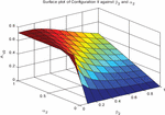
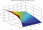
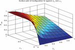
The purpose of this section is to see the impact of failure and repair rate on availability through surface plot using MATLAB software package. The results are summarized in Tables below.

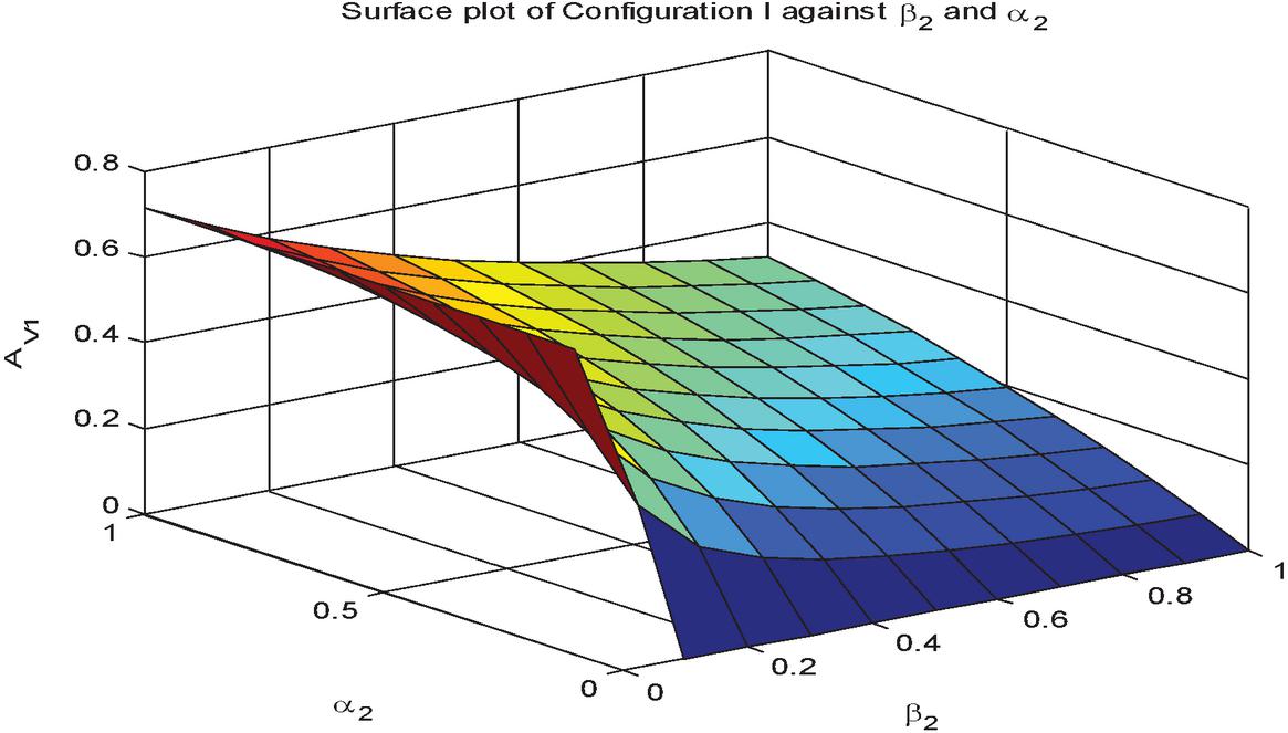
Figure 5a: Availability of Configuration I against ${\beta }_1$ and ${\alpha }_1$.

Figure 5b: Availability of Configuration I against ${\beta }_2$ and ${\alpha }_2$.

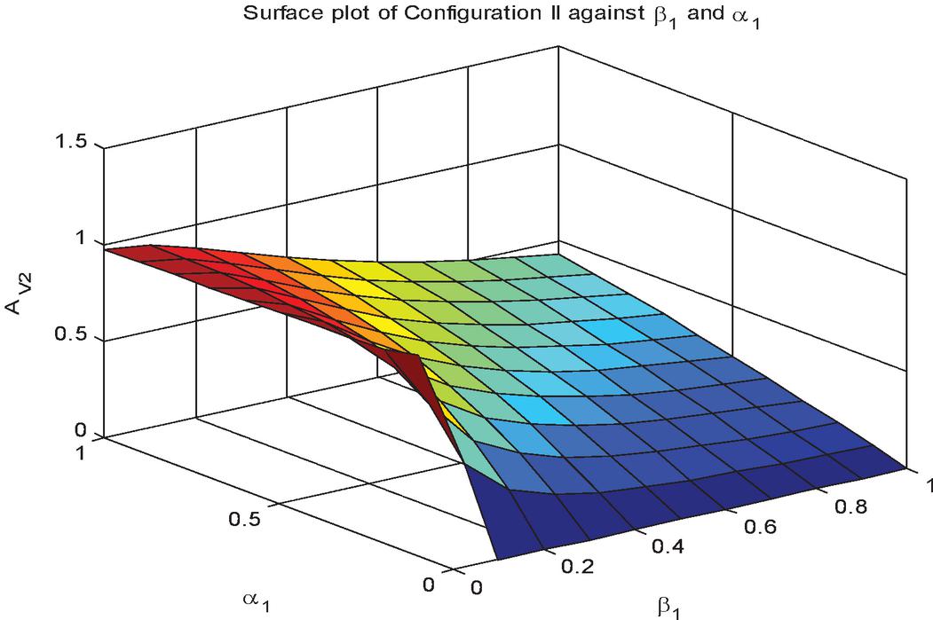
Figure 6a: Availability of Configuration II against ${\beta }_1$ and ${\alpha }_1$.

Figure 6b: Availability of Configuration II against ${\beta }_2$ and ${\alpha }_2$.

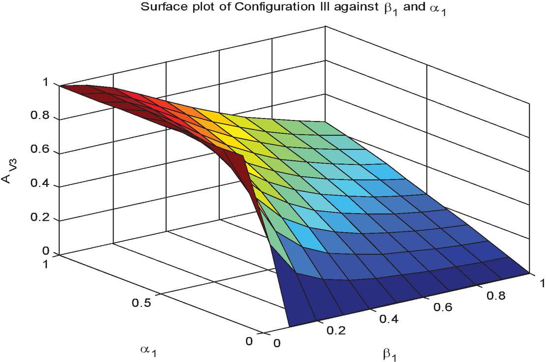
Figure 7a: Availability of Configuration III against ${\beta }_1$ and ${\alpha }_1$.

Figure 7b: Availability of Configuration III against ${\beta }_2$ and ${\alpha }_2$.

Figure 8a: Availability of Configuration IV against ${\beta }_1$ and ${\alpha }_1$.

Figure 8b: Availability of Configuration IV against ${\beta }_2$ and ${\alpha }_2$.

Figures 5a have shown the simulations of availability for Configuration I with respect to ${\alpha }_1$ and ${\beta }_1$. It is evident from this figure that availability increases with increase in ${\alpha }_1$ and decreases with increase in ${\beta }_1$. Similarly Figure 5b have shown the simulations of availability for Configuration I with respect to ${\alpha }_2$ and${\beta }_2$. It is clear from this figure that availability increases with increase in ${\alpha }_2$ and decreases with increase in ${\beta }_2$. It can be observe from these figures, that availability is higher with respect to the combination of ${\alpha }_1$ and ${\beta }_1$. This called for perfect repair with respect to ${\alpha }_2$ and major maintenance to reduce the occurrence of ${\beta }_2$. Simulation in Figures 6a and 6b revealed the impact of ${\alpha }_1$ and ${\beta }_1$ and the impact of ${\alpha }_2$ and ${\beta }_2$ on availability of Configuration II respectively. It is evident from these figures that availability increase with increase in ${\alpha }_1$ and ${\alpha }_2$, decreases with increase in ${\beta }_1$ and ${\beta }_2$ respectively. However, availability is higher in Figure 6a than Figure 6b.It is clear from this observation that the preventive maintenance and perfect repair should be invoke to control system degradation, fault and subsequent failures. On the other hand, simulations in Figures 7a to Figures 8b displayed similar pattern with Figures 5a to Figure 6b with respect to ${\alpha }_1$ and ${\beta }_1$, ${\alpha }_2$ and ${\beta }_2$ for Configuration III and Configuration IV.

It is evident from Figure 5a to Figure 8b, ${\beta }_2$ is the most critical to all configuration. Increase in ${\beta }_2$ decrease the values of availability for any configuration. To this effect, the configurations require adequate maintenance action in order to avoid catastrophic failure and prolong the life span of the configurations.

4.2 Ranking the Configurations based on their Availability

The purpose of this section is to rank the configurations for their availability using MATLAB software package. The results are summarized in Tables below.

Table 1 Ranking between the configurations in terms of their availability

Case	Parameter Range	Results	Constant values
1	$0<{\alpha }_1<0.1$	$A_{V1}(\mathrm{\infty })=A_{V2}(\mathrm{\infty })=A_{V3}(\mathrm{\infty })=A_{V4}(\mathrm{\infty })$	${\beta }_1=0.3$
	$0.1<{\alpha }_1<0.2$	$A_{V1}(\mathrm{\infty })<A_{V2}(\mathrm{\infty })=A_{V3}(\mathrm{\infty })<A_{V4}(\mathrm{\infty })$	${\beta }_2=0.03$
	$0.2<{\alpha }_1<0.3$	$A_{V1}(\mathrm{\infty })<A_{V2}(\mathrm{\infty })<A_{V3}(\mathrm{\infty })<A_{V4}(\mathrm{\infty })$	${\alpha }_2=0.4$
	$0.3<{\alpha }_1<0.4$	$A_{V1}(\mathrm{\infty })<A_{V2}(\mathrm{\infty })<A_{V3}(\mathrm{\infty })<A_{V4}(\mathrm{\infty })$
	$0.4<{\alpha }_1<0.5$	$A_{V1}(\mathrm{\infty })<A_{V2}(\mathrm{\infty })<A_{V3}(\mathrm{\infty })<A_{V4}(\mathrm{\infty })$
	$0.5<{\alpha }_1<0.6$	$A_{V1}(\mathrm{\infty })<A_{V2}(\mathrm{\infty })<A_{V3}(\mathrm{\infty })<A_{V4}(\mathrm{\infty })$
	$0.6<{\alpha }_1<0.7$	$A_{V1}(\mathrm{\infty })<A_{V2}(\mathrm{\infty })<A_{V3}(\mathrm{\infty })<A_{V4}(\mathrm{\infty })$
	$0.7<{\alpha }_1<0.8$	$A_{V1}(\mathrm{\infty })<A_{V2}(\mathrm{\infty })<A_{V3}(\mathrm{\infty })<A_{V4}(\mathrm{\infty })$
	$0.8<{\alpha }_1<0.9$	$A_{V1}(\mathrm{\infty })<A_{V2}(\mathrm{\infty })<A_{V3}(\mathrm{\infty })<A_{V4}(\mathrm{\infty })$
	$0.9<{\alpha }_1<1$	$A_{V1}(\mathrm{\infty })<A_{V2}(\mathrm{\infty })<A_{V3}(\mathrm{\infty })<A_{V4}(\mathrm{\infty })$

Table 2 Ranking between the configurations in terms of their availability

Case	Parameter Range	Results	Constant values
2	$0<{\beta }_1<0.1$	$A_{V1}(\mathrm{\infty })<A_{V2}(\mathrm{\infty })<A_{V3}(\mathrm{\infty })<A_{V4}(\mathrm{\infty })$	${\alpha }_1=0.7$
	$0.1<{\beta }_1<0.2$	$A_{V1}(\mathrm{\infty })<A_{V2}(\mathrm{\infty })<A_{V3}(\mathrm{\infty })<A_{V4}(\mathrm{\infty })$	${\beta }_2=0.03$
	$0.2<{\beta }_1<0.3$	$A_{V1}(\mathrm{\infty })<A_{V2}(\mathrm{\infty })<A_{V3}(\mathrm{\infty })<A_{V4}(\mathrm{\infty })$	${\alpha }_2=0.4$
	$0.3<{\beta }_1<0.4$	$A_{V1}(\mathrm{\infty })<A_{V2}(\mathrm{\infty })<A_{V3}(\mathrm{\infty })<A_{V4}(\mathrm{\infty })$
	$0.4<{\beta }_1<0.5$	$A_{V1}(\mathrm{\infty })<A_{V2}(\mathrm{\infty })<A_{V3}(\mathrm{\infty })<A_{V4}(\mathrm{\infty })$
	$0.5<{\beta }_1<0.6$	$A_{V1}(\mathrm{\infty })<A_{V2}(\mathrm{\infty })<A_{V3}(\mathrm{\infty })<A_{V4}(\mathrm{\infty })$
	$0.6<{\beta }_1<0.7$	$A_{V1}(\mathrm{\infty })<A_{V2}(\mathrm{\infty })<A_{V3}(\mathrm{\infty })<A_{V4}(\mathrm{\infty })$
	$0.7<{\beta }_1<0.8$	$A_{V1}(\mathrm{\infty })<A_{V2}(\mathrm{\infty })<A_{V3}(\mathrm{\infty })<A_{V4}(\mathrm{\infty })$
	$0.8<{\beta }_1<0.9$	$A_{V1}(\mathrm{\infty })<A_{V2}(\mathrm{\infty })<A_{V3}(\mathrm{\infty })<A_{V4}(\mathrm{\infty })$
	$0.9<{\beta }_1<1$	$A_{V1}(\mathrm{\infty })<A_{V2}(\mathrm{\infty })<A_{V3}(\mathrm{\infty })<A_{V4}(\mathrm{\infty })$

Table 3 Ranking between the configurations in terms of their availability

Case	Parameter Range	Results	Constant values
3	$0<{\alpha }_2<0.1$	$A_{V2}(\mathrm{\infty })<A_{V1}(\mathrm{\infty })<A_{V3}(\mathrm{\infty })<A_{V4}(\mathrm{\infty })$	${\beta }_1=0.3$
	$0.1<{\alpha }_2<0.2$	$A_{V1}(\mathrm{\infty })<A_{V2}(\mathrm{\infty })<A_{V3}(\mathrm{\infty })<A_{V4}(\mathrm{\infty })$	${\beta }_2=0.03$
	$0.2<{\alpha }_2<0.3$	$A_{V1}(\mathrm{\infty })<A_{V2}(\mathrm{\infty })<A_{V3}(\mathrm{\infty })<A_{V4}(\mathrm{\infty })$	${\alpha }_1=0.7$
	$0.3<{\alpha }_2<0.4$	$A_{V1}(\mathrm{\infty })<A_{V2}(\mathrm{\infty })<A_{V3}(\mathrm{\infty })<A_{V4}(\mathrm{\infty })$
	$0.4<{\alpha }_2<0.5$	$A_{V1}(\mathrm{\infty })<A_{V2}(\mathrm{\infty })<A_{V3}(\mathrm{\infty })<A_{V4}(\mathrm{\infty })$
	$0.5<{\alpha }_2<0.6$	$A_{V1}(\mathrm{\infty })<A_{V2}(\mathrm{\infty })<A_{V3}(\mathrm{\infty })<A_{V4}(\mathrm{\infty })$
	$0.6<{\alpha }_2<0.7$	$A_{V1}(\mathrm{\infty })<A_{V2}(\mathrm{\infty })<A_{V3}(\mathrm{\infty })<A_{V4}(\mathrm{\infty })$
	$0.7<{\alpha }_2<0.8$	$A_{V1}(\mathrm{\infty })<A_{V2}(\mathrm{\infty })<A_{V3}(\mathrm{\infty })<A_{V4}(\mathrm{\infty })$
	$0.8<{\alpha }_2<0.9$	$A_{V1}(\mathrm{\infty })<A_{V2}(\mathrm{\infty })<A_{V3}(\mathrm{\infty })<A_{V4}(\mathrm{\infty })$
	$0.9<{\alpha }_2<1$	$A_{V1}(\mathrm{\infty })<A_{V2}(\mathrm{\infty })<A_{V3}(\mathrm{\infty })<A_{V4}(\mathrm{\infty })$

Table 4 Ranking between the configurations in terms of their availability

Case	Parameter Range	Results	Constant values
4	$0<{\beta }_2<0.1$	$A_{V1}(\mathrm{\infty })<A_{V3}(\mathrm{\infty })<A_{V2}(\mathrm{\infty })<A_{V4}(\mathrm{\infty })$	${\beta }_1=0.3$
	$0.1<{\beta }_2<0.2$	$A_{V1}(\mathrm{\infty })<A_{V3}(\mathrm{\infty })<A_{V2}(\mathrm{\infty })<A_{V4}(\mathrm{\infty })$	${\alpha }_1=0.7$
	$0.2<{\beta }_2<0.3$	$A_{V1}(\mathrm{\infty })<A_{V3}(\mathrm{\infty })<A_{V2}(\mathrm{\infty })<A_{V4}(\mathrm{\infty })$	${\alpha }_2=0.4$
	$0.3<{\beta }_2<0.4$	$A_{V1}(\mathrm{\infty })<A_{V3}(\mathrm{\infty })<A_{V2}(\mathrm{\infty })<A_{V4}(\mathrm{\infty })$
	$0.4<{\beta }_2<0.5$	$A_{V1}(\mathrm{\infty })<A_{V3}(\mathrm{\infty })<A_{V2}(\mathrm{\infty })<A_{V4}(\mathrm{\infty })$
	$0.5<{\beta }_2<0.6$	$A_{V1}(\mathrm{\infty })<A_{V3}(\mathrm{\infty })<A_{V2}(\mathrm{\infty })<A_{V4}(\mathrm{\infty })$
	$0.6<{\beta }_2<0.7$	$A_{V1}(\mathrm{\infty })<A_{V3}(\mathrm{\infty })<A_{V2}(\mathrm{\infty })<A_{V4}(\mathrm{\infty })$
	$0.7<{\beta }_2<0.8$	$A_{V1}(\mathrm{\infty })<A_{V3}(\mathrm{\infty })<A_{V2}(\mathrm{\infty })<A_{V4}(\mathrm{\infty })$
	$0.8<{\beta }_2<0.9$	$A_{V1}(\mathrm{\infty })<A_{V3}(\mathrm{\infty })<A_{V2}(\mathrm{\infty })<A_{V4}(\mathrm{\infty })$
	$0.9<{\beta }_2<1$	$A_{V1}(\mathrm{\infty })<A_{V3}(\mathrm{\infty })<A_{V2}(\mathrm{\infty })<A_{V4}(\mathrm{\infty })$

Tables 1 to 4 depict the ranking of configuration base on their availability. It clear from the tables that configuration IV is the optimal configuration. Thus,

$A_{V1}(\mathrm{\infty })<A_{V3}(\mathrm{\infty })<A_{V2}(\mathrm{\infty })<A_{V4}(\mathrm{\infty })\mathit{\hspace{1em}}\text{for some }{\alpha }_k,{\beta }_k>0,$

$k=1,2.$

4.3 Sensitivity Analysis

This section presents the sensitivity analysis of the availability of each configuration with respect to variation in the values of input parameters.

(a) Case 1. By fixing ${\alpha }_2=0.4$, ${\beta }_2=0.03$, ${\alpha }_1=0.2$ and ${\alpha }_1=0.3$ varying ${\beta }_1$ as $0,0.1,0.2,0.3,\mathrm{\dots },0.9$, results of, $A_{V1}$, $A_{V2}$, $A_{V3}$ and $A_{V4}$ with respect to ${\beta }_1$ are presented in Table 5.

(b) Case 2. By fixing ${\alpha }_2=0.4$, ${\beta }_2=0.03$, ${\beta }_1=0.2$ and ${\beta }_1=0.3$ varying ${\alpha }_1$ as $0,0.1,0.2,0.3,\mathrm{\dots },0.9$, results of, $A_{V1}$, $A_{V2}$, $A_{V3}$ and $A_{V4}$ with respect to ${\alpha }_1$ are presented in Table 6.

(c) Case 3. By fixing ${\alpha }_1=0.7$, ${\beta }_1=0.3$, ${\alpha }_2=0.3$ and ${\alpha }_2=0.5$ varying ${\beta }_2$ as $0,0.1,0.2,0.3,\mathrm{\dots },0.9$, results of, $A_{V1}$, $A_{V2}$, $A_{V3}$ and $A_{V4}$ with respect to ${\beta }_2$ are presented in Table 7.

(d) Case 4. By fixing ${\alpha }_1=0.7$, ${\beta }_1=0.3$, ${\beta }_2=0.3$ and ${\beta }_2=0.5$ varying ${\beta }_1$ as $0,0.1,0.2,0.3,\mathrm{\dots },0.9$, results of, $A_{V1}$, $A_{V2}$, $A_{V3}$ and $A_{V4}$ with respect to ${\alpha }_2$ are presented in Table 8.

Table 5 Variation of availability of four configurations for different values of ${\alpha }_1$

	${\alpha }_1=0.2$				${\alpha }_1=0.3$
${\beta }_1$	$A_{V1}$	$A_{V2}$	$A_{V3}$	$A_{V4}$	$A_{V1}$	$A_{V2}$	$A_{V3}$	$A_{V4}$
0	0.9808	0.9912	0.9971	0.9808	0.9808	0.9928	0.9971	0.9808
0.1	0.6192	0.6712	0.6954	0.7392	0.7315	0.7908	0.8201	0.8621
0.2	0.4053	0.4298	0.4389	0.4624	0.5302	0.5679	0.5893	0.6265
0.3	0.2949	0.3081	0.3105	0.3229	0.4053	0.4286	0.4389	0.4624
0.4	0.2302	0.2383	0.2384	0.2459	0.3248	0.3402	0.3446	0.3598
0.5	0.1882	0.1936	0.1930	0.1979	0.2698	0.2805	0.2822	0.2926
0.6	0.1590	0.1628	0.1620	0.1655	0.2302	0.2381	0.2384	0.2459
0.7	0.1375	0.1404	0.1395	0.1421	0.2005	0.2054	0.2061	0.2117
0.8	0.1211	0.1233	0.1225	0.1245	0.1774	0.1821	0.1815	0.1858
0.9	0.1081	0.1099	0.1092	0.1107	0.1590	0.1628	0.1620	0.1655

Table 6 Variation of availability of four configurations for different values of ${\beta }_1$

	${\beta }_1=0.2$				${\beta }_1=0.3$
${\alpha }_1$	$A_{V1}$	$A_{V2}$	$A_{V3}$	$A_{V4}$	$A_{V1}$	$A_{V2}$	$A_{V3}$	$A_{V4}$
0	0	0	0	0	0	0	0	0
0.1	0.2302	0.2390	0.2384	0.2459	0.1590	0.1630	0.1620	0.1655
0.2	0.4053	0.4298	0.4389	0.4624	0.2949	0.3081	0.3105	0.3229
0.3	0.5302	0.5679	0.5893	0.6265	0.4053	0.4286	0.4389	0.4624
0.4	0.6192	0.6654	0.6954	0.7392	0.4933	0.5255	0.5446	0.5780
0.5	0.6836	0.7343	0.7689	0.8134	0.5632	0.6023	0.6291	0.6692
0.6	0.7315	0.7838	0.8201	0.8621	0.6192	0.6629	0.6954	0.7392
0.7	0.7678	0.8198	0.8565	0.8946	0.6643	0.7108	0.7473	0.7921
0.8	0.7961	0.8464	0.8830	0.9166	0.7011	0.7490	0.7880	0.8319
0.9	0.8186	0.8664	0.9027	0.9319	0.7315	0.7795	0.8201	0.8621

Table 7 Variation of availability of four configurations for different values of ${\alpha }_2$

	${\alpha }_2=0.3$				${\alpha }_2=0.5$
${\beta }_2$	$A_{V1}$	$A_{V2}$	$A_{V3}$	$A_{V4}$	$A_{V1}$	$A_{V2}$	$A_{V3}$	$A_{V4}$
0	0.7165	0.7165	0.8045	0.8045	0.7165	0.7165	0.8045	0.8045
0.1	0.5208	0.5952	0.5780	0.6624	0.5882	0.6835	0.6589	0.7368
0.2	0.3994	0.4411	0.4318	0.4988	0.4918	0.5978	0.5428	0.6256
0.3	0.3209	0.3416	0.3401	0.3882	0.4194	0.5072	0.4557	0.5270
0.4	0.2670	0.2776	0.2791	0.3142	0.3641	0.4318	0.3902	0.4489
0.5	0.2281	0.2336	0.2362	0.2627	0.3209	0.3276	0.3401	0.3882
0.6	0.1989	0.2017	0.2045	0.2251	0.2864	0.3263	0.3008	0.3405
0.7	0.1761	0.1775	0.1802	0.1966	0.2583	0.2896	0.2694	0.3025
0.8	0.1580	0.1585	0.1610	0.1744	0.2350	0.2601	0.2437	0.2717
0.9	0.1432	0.1432	0.1454	0.1566	0.2155	0.2359	0.2224	0.2463

Table 8 Variation of availability of four configurations for different values of ${\beta }_2$

	${\beta }_2=0.3$				${\beta }_2=0.5$
${\alpha }_2$	$A_{V1}$	$A_{V2}$	$A_{V3}$	$A_{V4}$	$A_{V1}$	$A_{V2}$	$A_{V3}$	$A_{V4}$
0	0	0	0	0	0	0	0	0
0.1	0.1432	0.1187	0.1454	0.1566	0.0914	0.0796	0.0920	0.0968
0.2	0.2461	0.2350	0.2559	0.2863	0.1666	0.1578	0.1700	0.1849
0.3	0.3209	0.3416	0.3401	0.3882	0.2281	0.2336	0.2362	0.2627
0.4	0.3766	0.4330	0.4050	0.4666	0.2788	0.3056	0.2923	0.3302
0.5	0.4194	0.5072	0.4557	0.5270	0.3209	0.3726	0.3401	0.3882
0.6	0.4531	0.5655	0.4961	0.5737	0.3562	0.4336	0.3810	0.4377
0.7	0.4801	0.6103	0.5288	0.6103	0.3861	0.4883	0.4161	0.4800
0.8	0.5023	0.6445	0.5556	0.6392	0.4117	0.5367	0.4465	0.5162
0.9	0.5208	0.6705	0.5780	0.6624	0.4338	0.5791	0.4729	0.5471

From sensitivity analysis presented in Table 5 for all configurations, one can observe that as ${\beta }_1$ increases from 0 to 0.9, the availability of all configurations decreases. Examination of the availability results of all configurations shown in this table reveals that configuration III has higher value of availability compared to other configurations initially for both ${\alpha }_1=0.2$ and ${\alpha }_1=0.3$. However, as the values of ${\beta }_1$ increases from 0.1 to 0.9, configuration IV has higher value of availability compared to other configurations. From the analysis in Table 5, it is clear that the contributing parameter toward the system performance is ${\alpha }_1$. This can be seen from the availability results of the configurations for ${\alpha }_1=0.2$ and ${\alpha }_1=0.3$. Thus, as ${\alpha }_1$ increases, so also the availability increase.

On the other hand, sensitivity analysis presented in Table 6 for all configurations, one can observe that as ${\alpha }_1$ increases from 0 to 0.9, the availability of all configurations increases also. Availability results of all configurations displayed in this table reveals that configuration IV has higher value of availability compared to other configurations initially for both ${\beta }_1=0.2$ and ${\beta }_1=0.3$. However, as the values of ${\beta }_1$ changes from 0.2 to 0.3, availability of all configurations decreases. Nonetheless, configuration IV remains the optimal configuration. ${\beta }_1$ can be viewed as the parameter contributing the decrease in the performance of the configurations.

Sensitivity analysis displayed in Table 7 for all configurations have shown that availability decreases with increase ${\beta }_2$ increases from 0 to 0.9 as ${\alpha }_2$ changes from 0.3 to 0.5 with configuration IV having the highest value of availability compared to other configurations. From the analysis it is clear that the performance of the system can be improve whenever ${\alpha }_2\ge 0.3$.

From the sensitivity analysis shown in Table 8 for all configurations, it is evident that as ${\alpha }_2$ increases from 0 to 0.9, the availability of all configurations increases also. Availability results of all configurations displayed in this table reveals that configuration IV has higher value of availability compared to other configurations whenever $0\le {\alpha }_2\le 0.7$ when ${\beta }_2$ changes from 0.3 to 0.5. However, as the values of ${\alpha }_2$ from 0.8 to 0.9, configuration II has higher value of availability compared to other configurations.

It evident from Tables 5 and 7 that availability decreases as ${\beta }_1$ and ${\beta }_2$ increase. The analysis has shown that Configuration IV has higher availability than the remaining configurations for each ${\alpha }_1\in [0.2,0.3]$ and ${\alpha }_2\in [0.3,0.5]$. Similarly, sensitivity analysis in Tables 6 and 8 have shown that availability increases as ${\alpha }_1$ and ${\alpha }_2$ increase. However, availability of Configuration IV is higher in these tables than the remaining configuration for each ${\beta }_1\in [0.2,0.3]$ and ${\beta }_2\in [0.3,0.5]$.

4.4 Partial Rank Correlation Coefficients (PRCC)

This section used the partial rank correlation coefficient of the availability of each configuration in order to determine the most critical parameter that may lead to decrease in the availability using MATLAB package. The experiments are presented below:

Figure 9 Tornado plot of Configuration I.

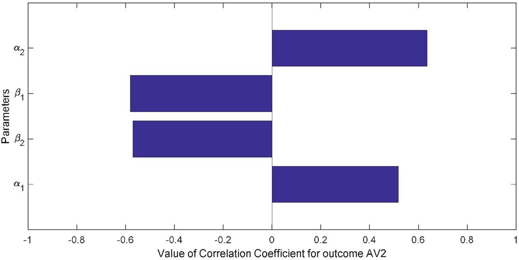
Figure 10 Tornado plot of Configuration II.

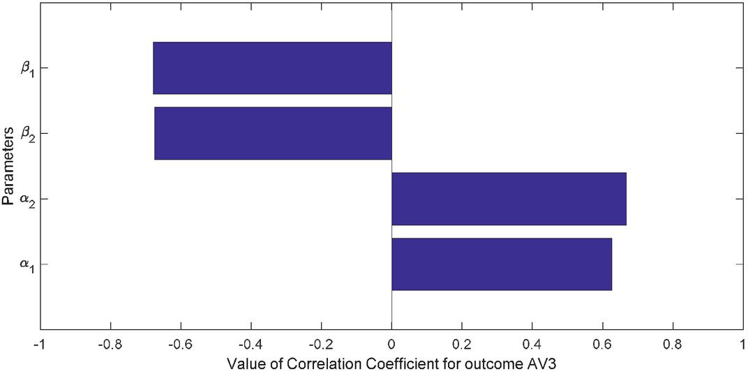
Figure 11 Tornado plot of Configuration III.

Figure 12 Tornado plot of Configuration IV.

We conducted sensitivity analysis on ${\beta }_k$ and ${\alpha }_k$, $k=1,2$ to measure their statistical influence on $A_{V1}$ to $A_{V4}$. To do that each ${\beta }_k$ and ${\alpha }_k$ is uniformly distributed on [0 1] and we draw 1000 samples from this distribution using Latin Hypercube sampling. This gives a matrix with 1000 rows 5 columns. Each row of the matrix represents a unique parameter set. For each of these sets, we simulated the model outcomes of availability $A_{V1}$ to $A_{V4}$. We then performed sensitivity analysis on the model outcomes using partial rank correlation coefficients (PRCC). Figures 5 to 8 depicts the tornado plots of the results. From the Figures 9 to 12, it is evident that ${\alpha }_2$ is the most sensitive parameter affecting all the outcomes ($A_{V1}$ to $A_{V4}$). Increase in ${\alpha }_2$ will lead to increase in the outcomes. The PRCC results for ${\beta }_1$ are similar in the Figures 9 to 11. The results indicate that ${\beta }_1$ is the most sensitive, while ${\beta }_2$ is the least sensitive for all the outcomes in the Figures 9 to 12. Increasing the value of ${\beta }_1$ will decrease each one of the outcomes more significantly than the other. The PRCC results for ${\beta }_2$ depicted in Figures 12. The results in this Figure indicates that ${\beta }_2$ is the most sensitive, while ${\beta }_1$ is the least sensitive for all the outcomes in the Figures 12. Increasing the value of ${\beta }_2$ will decrease each one of the outcomes more significantly than the other ${\beta }_1$. These means that in order to have high values of availability of the configurations I to IV, it is necessary to consider the combinations of high values of ${\alpha }_2$ together with low values of ${\beta }_1$ and ${\beta }_2$ in the Figures 9 to 12. This means that processors should be given more care in terms of maintenance.

5 Conclusion

This paper studied availability of four hybrid systems configured as series-parallel systems in which each system or configuration consisting of main units and their corresponding processors in the form of k-out-of-n system. Explicit expression for the steady-state availability is derived and validated by performing numerical experiments. Analysis of the effect of various system parameters on availability was performed through MATLAB surface plot and tornado plot. These are the main contribution of the paper. From the surface plot presented in the study, it can be concluded that maintenance strategies that will keep the system as failure free should be invoke to maximize availability, product quality, and production output and revenue generation. The present work can be extended further for a system to connect to multi standby devices. On the basis of the tornado plot obtained in Figures 9–12 and ranking in Tables 1–4, it is evident that the availability can be enhanced through high value of ${\alpha }_2$ together with low values of ${\beta }_1$ and ${\beta }_2$. Thus, the processors should be given priority in terms of maintenance. From the analysis, it is evident that availability can be enhancing through, proper maintenance planting to avoid the occurrence of catastrophic failure, maintaining the system availability at the highest order through high value of ${\alpha }_2$ and low value of ${\beta }_1$ and ${\beta }_2$, by adding fault tolerant units and processors. The present work can be extended further for a system to connect to multi-processor and solve using supplementary variable techniques.

References

[1] Aliyu, M.S., Yusuf, I. and Ali, U.A. (2015) ‘Availability and profit optimazation of series-parallel system with linear consecutive cold standby unit’, Applied Mathematics, 6(2), 332–344. DOI: 10.4236/am.2015.62032

[2] Bhardwaj, R.K. and Chander, S. (2007). Reliability and cost benefit analysis of 2-out-of-3 redundant system with general distribution of repair and waiting time. DIAS- Technology review- An Int. J. of business and IT. 4(1), 28–35.

[3] Bhardwaj, R. K and Malik, S. C. (2010), MTSF and cost effectiveness of 2-out-of-3standby system with probability of repair and inspection. International Journal ofEngineering Science and Technology, 2(1): 5882-5889.

[4] Chander, S. and Bhardwaj, R.K. (2009). Reliability and economic analysis of 2-out-of-3 redundant system with priority to repair. African J. of Maths and comp. sci, 2(11), 230–236.

[5] Chander, S. and Bhardwaj, R.K. (2009). Reliability and economic analysis of 2-out-of-3 redundant system with priority and replacement. Decision and Mathematical sciences, 10(1–3), 79–100.

[6] Chander, S. and Bhardwaj, R.K. (2009). Reliability modelling and analysis of 2-out-of-3 redundant system subject to conditional arrival time of server. Proc. 13th ISSAT INC. on RQD, seattle (USA), 206–210.

[7] Garg, H. (2014). Reliability, availability and maintainability analysis of industrial systems using PSO and fuzzy methodology. MAPAN, 29(2), 115–129. DOI: 10.1007/s12647-013-0081-x

[8] Garg, H. (2016). A novel approach for analyzing the reliability of series-parallel system using credibility theory and different types of intuitionistic fuzzy numbers. Journal of the Brazilian Society of Mechanical Sciences and Engineering, 38(3), 1021–1035. DOI: 10.1007/s40430-014-0284-2

[9] Garg, H. (2016). An approach for analyzing the reliability of industrial system using fuzzy kolmogrov’s differential equations. Arabian Journal for Science and Engineering, 40(3), 975–987. DOI: 10.1007/s13369-015-1584-2

[10] Garg, H. (2017). Performance analysis of an industrial system using soft computing based hybridized technique, J Braz. Soc. Mech. Sci. Eng. 39:1441–1451 DOI 10.1007/s40430-016-0552-4

[11] Khatab, A., Nahas, N., and Nourelfath, M., (2009). Availbilty of k-out-of-n: G systems with non identical components subject to repair priorities.Reliab. Eng. Syst. Safety. 94, 142–151. DOI: 10.1016/j.ress.2008.02.017

[12] Kumar, A., Singh, S.B. and Ram, M. (2020). Systems reliability assessment using hesitant fuzzy set, International Journal of Operational Research, 38(1), 1–18.

[13] Li, X., Zuo, M.J. and Yam, R.C. (2006). Reliability analysis of a repairable k-out-of-n system with some components being suspended when the system is down. Reliab Eng. Syst. Safety. 91, 305–310.

[14] Niwas, R. and Garg, H. (2018). ‘An approach for analyzing the reliability and profit of an industrial system based on the cost-free warranty policy.’ Journal of the Brazilian Society of Mechanical Sciences and Engineering, 40: 265. DOI: 10.1007/s40430-018-1167-8

[15] Singh, V.V and Rawal, D.K. (2015). ‘Availability, MTTF, and cost analysis of the complex system under preemptive resume repair policy using copula distribution,’ Journal of Statistics and Operation Research Vol. 10(3), pp. 299–321. DOI:10.18187/pjsor.v10i3.724

[16] Yusuf, I and Hussaini N. (2012). Evaluation of reliability and availability characteristics of 2-out-3 standby system under a perfect repair condition. American Journal of Mathematics and Statistics, 2(5): 114–119. doi: 10.5923/j.ajms.20120205.03

[17] Yusuf, I., Babagana, M., Yusuf, B. and Lawan, M.A. (2014). Reliability Analysis of a Linear consecutive 2-out-of-3 System in the presence of Supporting Device and Repairable Service Station. International Journal of operation research, 13(1): 013–024. DOI: 10.21307/ijor-2016-002

[18] Yusuf, I. (2016). ‘Reliability Modeling of a Parallel System with a Supporting Device and Two Types of Preventive Maintenance,’ International journal of operational Research Vol. 25(3), pp. 269–287. DOI: 10.1504/IJOR.2016.074754

Biographies

Ibrahim Yusuf is an Associate Professor in the Department of Mathematical Sciences, Bayero University Kano, Nigeria. He obtained his PhD in the University of Bayero University Kano, Nigeria. He has taught in BUK for more than 18 years. He is currently the Dean Faculty of Computer Science and Information Technology, Bayero University Kano, Nigeria. His research interest includes operation research, stochastic analysis, statistics and reliability modelling. He has published a number of research articles in both local and international journals.

Nafisa Muhammad Usman is a lecturer in the Department of Arts and Humanity, School of General Studies, Kano State Polytechnic, Kano, Nigeria. She received her M.Sc in Mathematics the Department of Mathematical Sciences, Bayero University Kano, Nigeria. She is currently a Phd candidate in the Department of Mathematical Sciences, Bayero University Kano, Nigeria. She has 8 years of teaching and research experience. Her research interest includes operation research and reliability.

Saminu Iliyasu Bala is a Professor in the Department of Mathematical Sciences, Bayero University Kano, Nigeria.He obtained his B.Sc and M.Sc degree in Mathematics from Bayero University Kano, Nigeria. Mr Bala obtained his PhD from the University of Liverpool in the year 2009. He has since been lecturer in Bayero University Kano where he supervised and still supervising many students.

Journal of Reliability and Statistical Studies, Vol. 13_2-4, 429–460.
doi: 10.13052/jrss0974-8024.132411
© 2021 River Publishers