Algebraic and Geometric Basis of Principal Components: An Overview

Pramit Pandit*, K. N. Krishnamurthy and K. B. Murthy

Department of Agricultural Statistics, Applied Mathematics and Computer Science, University of Agricultural Sciences, Bengaluru, Karnataka, India

E-mail: pramitpandit@gmail.com; kkmurthy13@gmail.com; kbmurthy2005@gmail.com

*Corresponding Author

Received 21 May 2019; Accepted 10 June 2020; Publication 13 October 2020

Abstract

Principal Component Analysis is considered as a dimension-reduction tool which may be used to reduce a large set of possibly correlated variables to hopefully a smaller set of uncorrelated variables that still accounts for most of the variation of the original large set. To understand the inner constructs of principal components, concepts of algebraic as well as geometric basis of principal components are prerequisites. Hence, in the current study, an attempt has been made to provide a step by step and vivid discussion of the basis of principle components and its various important properties.

Keywords: Algebraic basis, basis of principal components, geometric basis, principal components, properties of principal components.

1 Introduction

Principal component analysis (PCA) is a statistical method in which an orthogonal transformation is used to convert a set of observations of possibly correlated variables into a (hopefully, smaller) set of observations of linearly uncorrelated variables, called principal components (Jackson, 1991; Harris, 2001). The method of principal components was given by Karl Pearson in the year of 1901 (Pearson, 1901), however the general procedure being used nowadays is due to Harold Hotelling, whose pioneering paper showed up later in 1933 (Hotelling, 1933). This transformation is defined such that the first principal component has the largest possible variance and accounts for as much of the variability present in the original data as possible (Anderson, 2003; Johnson and Wichern, 2007). Each succeeding principal component in turn has the next highest possible variance under the constraint that it is orthogonal to the preceding principal component(s) so that the resulting vectors become an uncorrelated orthogonal basis set (Hardle and Simar, 2014). In regression analysis, a test without principal component analysis may be ineffective or even impossible if the number of independent variables is large compared to the number of observations (Timm, 2002). Besides, substantially higher correlations among the independent variables may lead to unstable estimates of regression coefficients (Gujarati et al., 2011). In such cases, these variables can be reduced to a smaller number of principal components resulting in a better test or more stable estimates of regression coefficients (Rencher, 2012). In case of MANOVA, if p (number of dimensions) is close to ${\nu }_E$ (error degrees of freedom) so that a test has a low power, or that, $\mathrm{p}>{\nu }_E$, making the determinants of Wilks’ $\mathrm{\Lambda }$ negative, the dependent variables should be substituted with a smaller number of principal components in order to carry out the analysis (Rencher, 2012). In addition to these applications, depending on the fields, it is analogous to the discrete Karhunen–Loève transform in signal processing (Ahmed et al., 1974), proper orthogonal decomposition in mechanical engineering (Chatterjee, 2000), singular value decomposition in linear algebra (Bunch and Nielsen, 1978), Eckart–Young theorem in psychometrics (Johnson, 1963), empirical orthogonal functions in meteorological sciences (Hannachi et al., 2007) and so on. It should be noted that in the term principal components, the adjective ‘principal’ is used to describe the kind of components – main, primary, fundamental, major, and so on. The noun ‘principal’ as a modifier for components, is not used (Rencher, 2012). To understand the inner constructs of principal components, concepts of algebraic as well as geometric basis of principal components are prerequisites. Hence, in the current study, an attempt has been made to provide a step by step and vivid discussion of the basis of principle components and its various importantproperties.

2 Algebraic Basis of Principal Components

Let $\overrightarrow{X}$ be an n-dimensional vector of variables and n is assumed to be very large. Now the interest is emphasized on reducing this n number of variables (may be correlated) into m ($\mathrm{m}\le \mathrm{n}$) number of uncorrelated variables (Rencher, 2012).

$$\overrightarrow{X}=(X_1,X_2,X_3,\mathrm{\dots }{X}_m,X_{m+1},\mathrm{\dots },X_n)$$

In other words, (n-m) number of variables have to be deleted in order to decrease redundancy. Now, if the first m number of variables are kept by eliminating the last (n-m) number of variables, it will contribute sufficient increase in error sum of squares, as here, the condition $\mathrm{V}(X_1)\ge \mathrm{V}(X_2)\ge \mathrm{\dots }\mathrm{V}(X_m)\gg \mathrm{V}(X_{m+1})\ge \mathrm{\dots }\mathrm{V}(X_n)$ is not ascertained. So, to ensure the condition $\mathrm{V}(X_1)\ge \mathrm{V}(X_2)\ge \mathrm{\dots }\mathrm{V}(X_m)\gg \mathrm{V}(X_{m+1})\ge \mathrm{\dots }\mathrm{V}(X_n),$ transformation of $\overrightarrow{X}$ vector is obvious. Now, a way of transformation of the $\overrightarrow{X}$ vector has to be thought of in such a way that the aforesaid variability condition is ascertained to ensure minimum increase in error sum of squares if the last (n-m) variables are eliminated. In other words, the objective of this transformation is to maximise the decrease of variance so that the last (n-m) number of variables can be easily chopped off.

First of all, let $\overrightarrow{q}$ be an n-dimensional unit vector. So, by definition, Euclidian norm of $\overrightarrow{q}$ vector, $\parallel \overrightarrow{q}\parallel =1$.

Now, a projection of $\overrightarrow{X}$ vector onto the n-dimensional unit vector $\overrightarrow{q}$ has been made.

$\therefore$ Projection of $\overrightarrow{X}$ onto $\overrightarrow{q}$, $\mathrm{C}={\overrightarrow{X}}^T\overrightarrow{q}={\overrightarrow{q}}^T\overrightarrow{X}$  (Stark and Yang, 1998), which is subjected to $\parallel \overrightarrow{q}\parallel ={({\overrightarrow{q}}^T\overrightarrow{q})}^{1/2}=1$.

Again, $\mathrm{V}(\mathrm{C})={\overrightarrow{q}}^{T}S\overrightarrow{q}$, where S is the sample variance-covariance matrix of variables of $\overrightarrow{X}$ vector. This matrix S is beyond researchers’ control. So what can be done is that this n-dimensional unit vector $\overrightarrow{q}$ can be utilised as a search to get the desired form.

Let variance probe,

$$\mathrm{\Psi }\left(\overrightarrow{q}\right)={\overrightarrow{q}}^{T}S\overrightarrow{q}={\sigma }^2$$

(1)

Now, as a corollary to Rolle’s Mean Value theorem (Riedel and Sahoo, 1998), for a very small change $\overrightarrow{\delta q}$ , $\mathrm{\Psi }(\overrightarrow{q})$ can be approximated to $\mathrm{\Psi }(\overrightarrow{q}+\overrightarrow{\delta }q)$, i.e.

$$\mathrm{\Psi }\left(\overrightarrow{q}\right)=\mathrm{\Psi }(\overrightarrow{q}+\overrightarrow{\delta }q)$$

(2)

From (1), $\mathrm{\Psi }(\overrightarrow{q}+\overrightarrow{\delta }q)={(\overrightarrow{q}+\overrightarrow{\delta }q)}^{T}S(\overrightarrow{q}+\overrightarrow{\delta }q)$

	$=$	${\overrightarrow{q}}^{T}S\overrightarrow{q}+2\overrightarrow{\delta }{q}^{T}S\overrightarrow{q}+\overrightarrow{\delta }{q}^{T}S\overrightarrow{\delta }q$	(3)
	$=$	${\overrightarrow{q}}^{T}S\overrightarrow{q}+2\overrightarrow{\delta }{q}^{T}S\overrightarrow{q}$

(As the quantity $\overrightarrow{\delta }{q}^{T}S\overrightarrow{\delta }q$ is infinitely small)

Putting the value of (1) and (3) in (2),

$${\overrightarrow{q}}^{T}S\overrightarrow{q}={\overrightarrow{q}}^{T}S\overrightarrow{q}+2\overrightarrow{\delta }{q}^{T}S\overrightarrow{q}$$

Or,

$$\overrightarrow{\delta }{q}^{T}S\overrightarrow{q}=0$$

(4)

Now, as $\overrightarrow{q}$ is an unit vector, even after perturbation, $(\overrightarrow{q}+\overrightarrow{\delta }q)$ also remains as an unit vector.

$$\therefore \parallel (\overrightarrow{q}+\overrightarrow{\delta }q)\parallel =1$$

Squaring both sides, it can be obtained that

$${\parallel (\overrightarrow{q}+\overrightarrow{\delta }q)\parallel }^2=1$$

Or,

$${\left(\overrightarrow{q}+\overrightarrow{\delta }q\right)}^T\left(\overrightarrow{q}+\overrightarrow{\delta }q\right)=1$$

Or,

$${\overrightarrow{q}}^T\overrightarrow{q}+2\overrightarrow{\delta }{q}^T\overrightarrow{q}+\overrightarrow{\delta }{q}^T\overrightarrow{\delta }q=1$$

Or,

$$\overrightarrow{\delta }{q}^T\overrightarrow{q}=0$$

(5)

(As the quantity $\overrightarrow{\delta }{q}^T\overrightarrow{\delta }q$ is infinitely small and ${\overrightarrow{q}}^T\overrightarrow{q}=1$ for $\overrightarrow{q}$ being an unit vector).

Now, using Lagrangian multiplier $\lambda$ (Bertsekas, 2014), from (4) and (5),

$$\overrightarrow{\delta }{q}^{T}S\overrightarrow{q}-\lambda \left(\overrightarrow{\delta }{q}^T\overrightarrow{q}\right)=0$$

Or,

$$\overrightarrow{\delta }{q}^T\left[S\overrightarrow{q}-\lambda \overrightarrow{q}\right]=0$$

As this $\overrightarrow{\delta }{q}^T$ is certainly a non-zero quantity, so

$$\left[S\overrightarrow{q}-\lambda \overrightarrow{q}\right]=0$$

Or,

$$\left[\mathrm{S}-\mathrm{I}\lambda \right]\overrightarrow{q}=0$$

(6)

where I is nxn identity matrix.

Now, this Equation (6) is a well-known form in linear algebra (Zhang, 2011), more specifically in matrix theory, where $\lambda$ is the eigen value of S matrix and $\overrightarrow{q}$ is the corresponding eigen vector (Searle and Khuri, 2017). As S is a square matrix of order n, there will be n number of eigen values and n corresponding eigen vectors. Arranging eigen values in the decreasing order (i.e. ${\lambda }_1\ge {\lambda }_2\ge \mathrm{\dots }{\lambda }_m\ge {\lambda }_{m+1}\ge \mathrm{\dots }{\lambda }_n)$, it can be obtained (Johnstone, 2001),

$$S{\overrightarrow{q}}_j={\lambda }_j{\overrightarrow{q}}_j\mathit{\hspace{1em}}(\mathrm{where},\mathrm{j}=1,2,\mathrm{\dots },\mathrm{n})$$

(7)

Now, two matrices Q and $\mathrm{\Delta }$ are defined as $Q=[{\overrightarrow{q}}_1,{\overrightarrow{q}}_2,{\overrightarrow{q}}_3,\mathrm{\dots },{\overrightarrow{q}}_n]$ and $\mathrm{\Delta }=\mathrm{diag}({\lambda }_1,{\lambda }_2,{\lambda }_3,\mathrm{\dots },{\lambda }_n)$, respectively. Compacting the n number of Equations (7) in a single equation, it can be obtained,

$$SQ=Q\mathrm{\Delta }$$

(8)

Again, ${\overrightarrow{q}}_1,{\overrightarrow{q}}_2,{\overrightarrow{q}}_3,\mathrm{\dots },{\overrightarrow{q}}_n$ are eigen vectors of S matrix. As variance-covariance matrix S is a symmetric matrix, its eigen vectors are orthogonal to each other. Hence, matrix Q, consisting of n-orthogonal eigen vectors, is an orthogonal matrix, satisfying

$\overrightarrow{q}_j{}^T{\overrightarrow{q}}_i$	$=1,\mathrm{for}\mathit{\hspace{1em}}i=j$
	$=0,\mathrm{for}\mathit{\hspace{1em}}i\ne j$

and

$$Q^{T}Q=I\mathit{\hspace{1em}}\mathrm{i}.\mathrm{e}.\mathit{\hspace{1em}}{Q}^T=Q^{-1}.$$

Pre-multiplying $Q^T$ to both the sides of (8),

$$Q^{T}SQ=\mathrm{\Delta }$$

(9)

and an expanded form of this Equation (9) will be

$\overrightarrow{q}_j{}^{T}S{\overrightarrow{q}}_k$	$=$	${\lambda }_j,\mathrm{for}\mathit{\hspace{1em}}k=j$ (10)
	$=$	$0,\mathrm{for}\mathit{\hspace{1em}}k\ne j$

As the left hand side of the Equation (9) is similar to the Equation (1) as mentioned earlier, Variance-Covariance matrix of transformed vector C will be,

$$(\mathrm{i})\sum =\mathrm{\Delta }$$

(11)

From equality property of matrices (Aitken, 2016), the following properties can be obtained,

$$(\mathrm{ii}){\sigma }_{ij}={\lambda }_i,\mathrm{for}\mathit{\hspace{1em}}i=j$$

(12)

$$=0,\mathrm{for}\mathit{\hspace{1em}}i\ne j,$$

$$(\mathrm{iii})\sum _{i=1}^n{\sigma }_{ij}=\sum _{i=1}^n{\lambda }_i$$

(13)

and

$$(\mathrm{iv})\mathit{\hspace{1em}\hspace{1em} }\mathrm{proportion}\mathrm{of}\mathrm{variability}\mathrm{explained}\mathrm{by}{i}^{\mathrm{th}}\mathrm{PC}=\frac{{\lambda }_i}{{\sum }_{i=1}^n{\lambda }_i}$$

(14)

3 Geometric Basis of Principal Component

Suppose for 2 variables ${\mathrm{X}}_1$ and ${\mathrm{X}}_2$, the following scatterplot has been obtained (Figure 1).

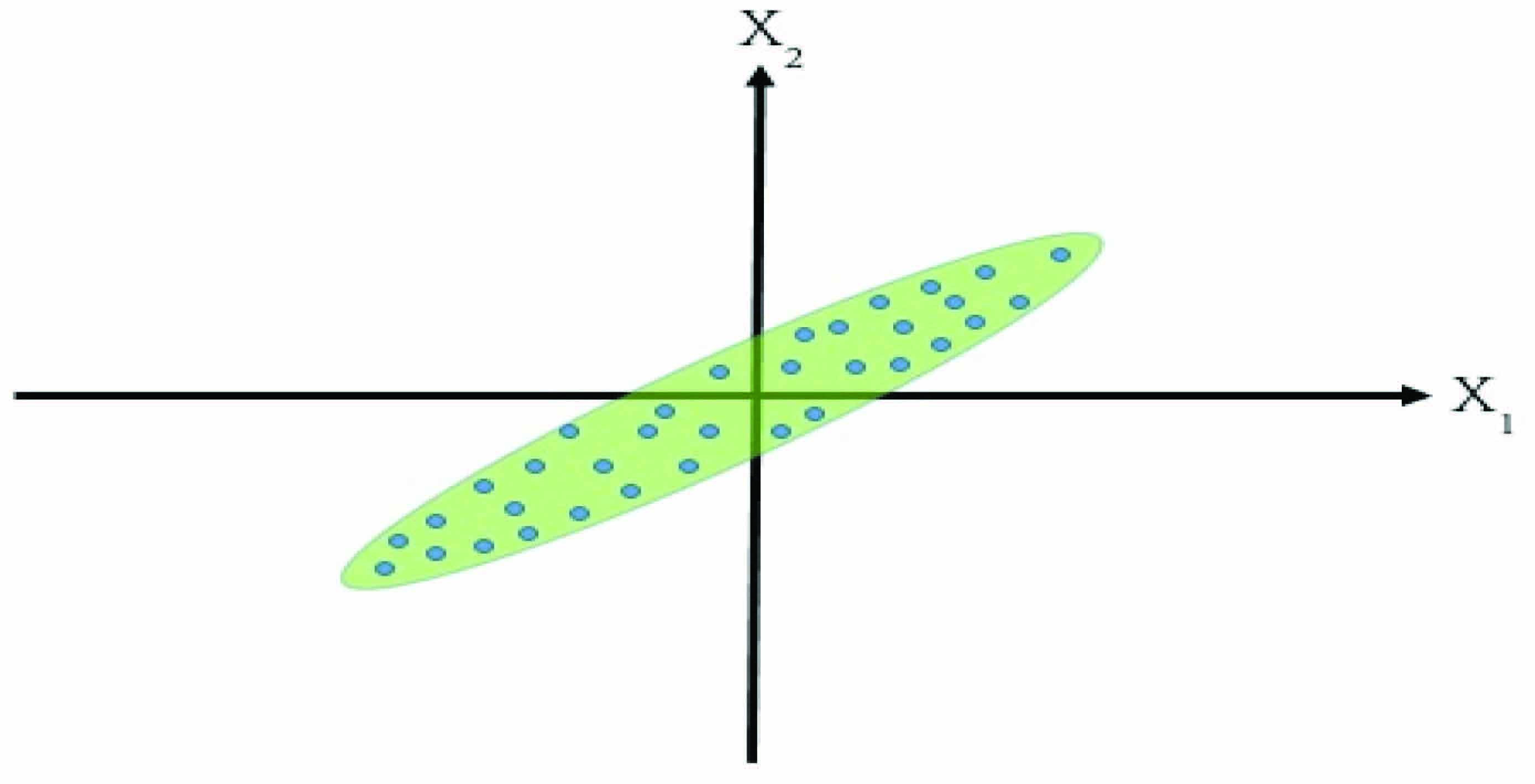
Figure 1 Scatterplot of X${}_1$ and X${}_2$ variable.

Now, from the scatterplot (Figure 1), it can be clearly understood that $X_1$ and $X_2$ are highly correlated. It can also be observed that variability across $X_1$ is higher than variability across $X_2$, however both are substantial values (Figure 2).

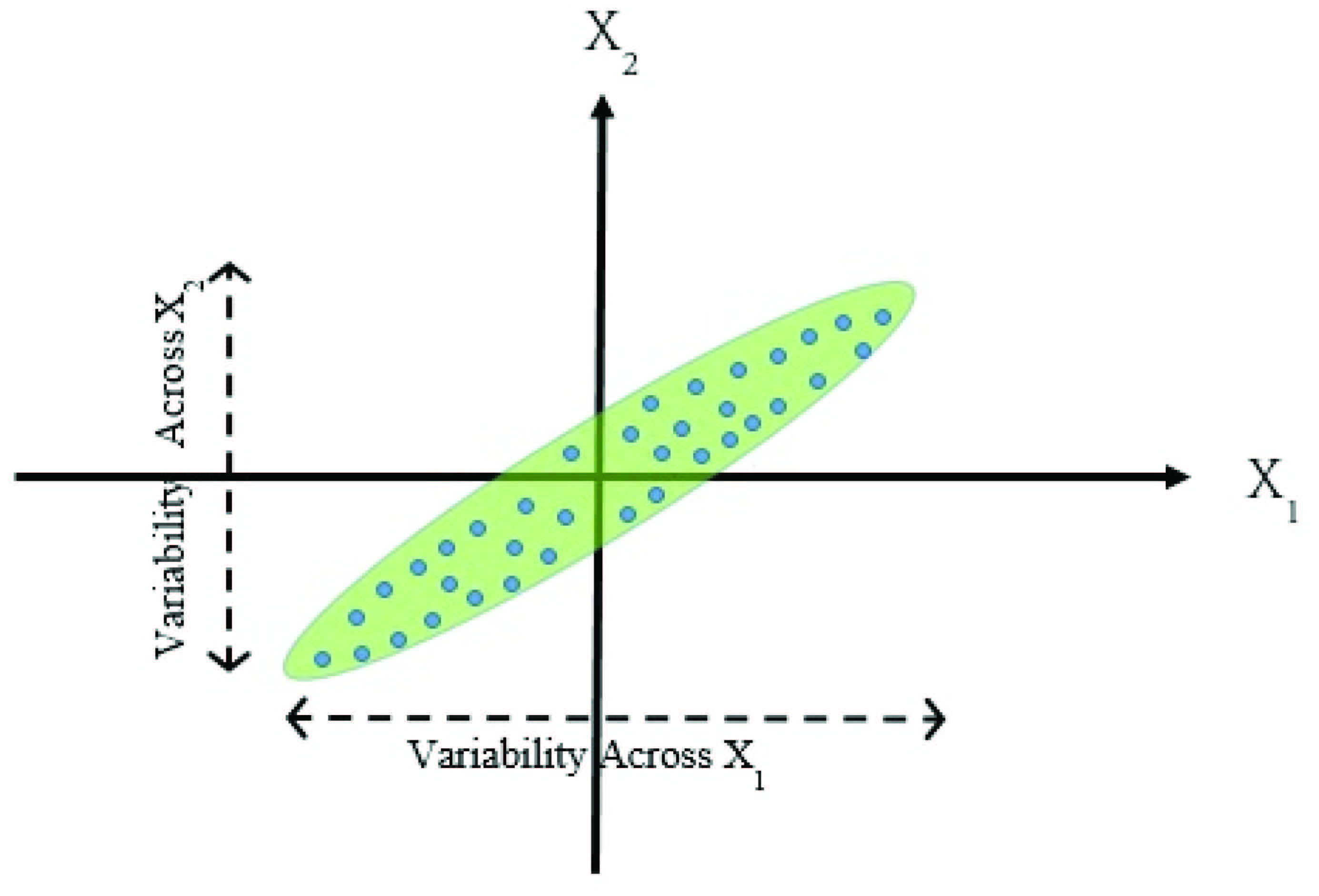
Figure 2 Variability across X${}_1$ and X${}_2$ axis in the scatterplot.

Keeping the origin rigid, if the axes are rotated ${\mathrm{\theta }}^0$ anti-clockwise (Figure 3), the rotation will yield $Z_1$, $Z_2$ as new axes (Eisenhart, 2005).

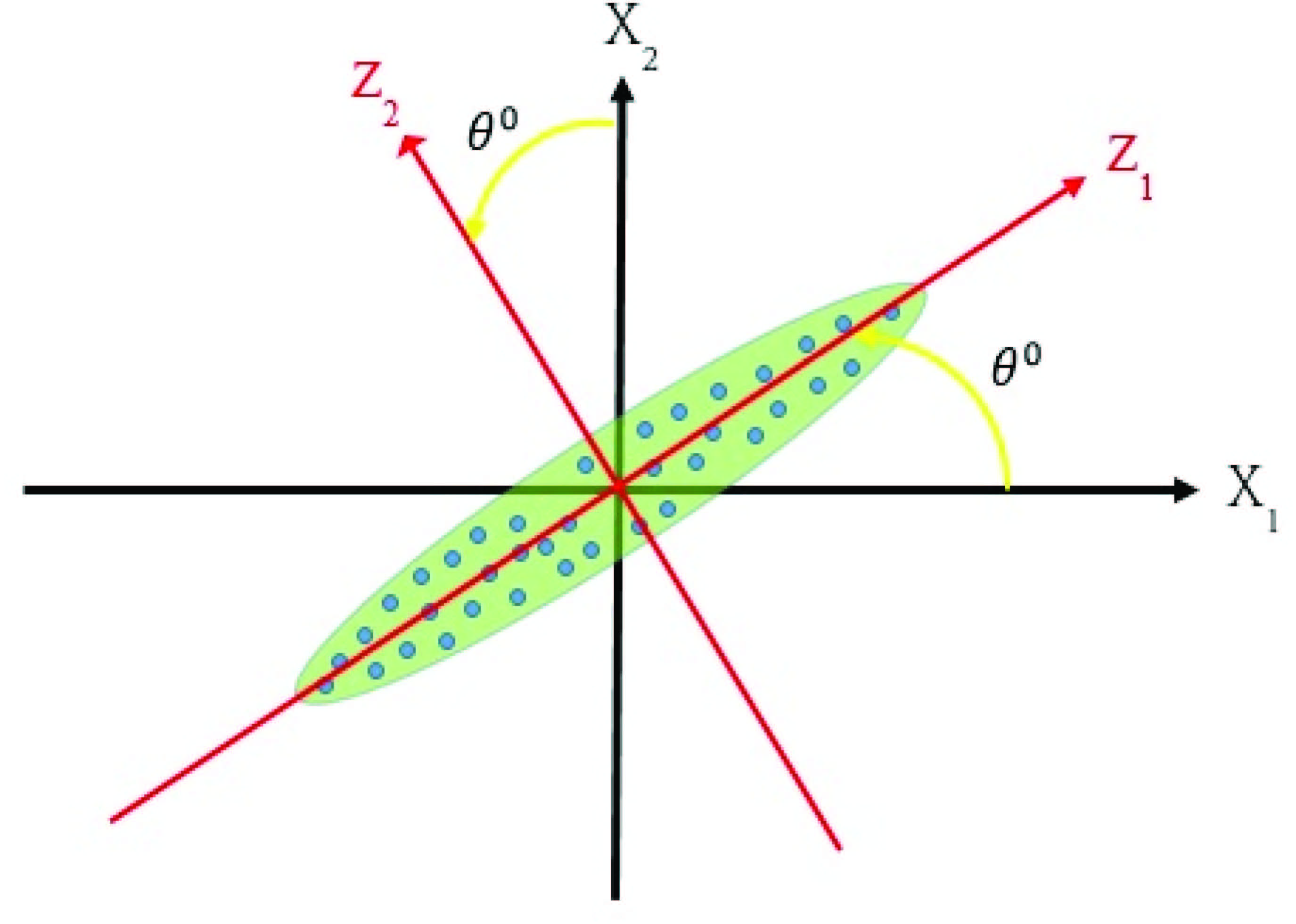
Figure 3 Rotated scatterplot of X${}_1$ and X${}_2$ variable.

After rotation, it can be seen that variability across $Z_1$ is much higher than $Z_2$. In addition to that, $Z_1$ and $Z_2$ are observed to be almost independent. Now, if $\mathrm{V}(Z_1)\gg \mathrm{V}(Z_2)$, then $Z_1$ dimension alone will be able to provide sufficient information as much as available in the original data set.

Now, a particular point P is considered, whose coordinate is ($x_1$, $x_2$) in $X_1{X}_2$ plane and ($z_1$, $z_2$) in $Z_1{Z}_2$ plane (Figure 4). From P, perpendicular lines PM and PA have been drawn on $Z_1$ axis and $Z_2$ axis respectively. From P, another perpendicular line PL has been drawn on $X_1$ axis. From the point M, two perpendicular line MQ and MN have been drawn on $X_1$ axis and PL line, respectively.

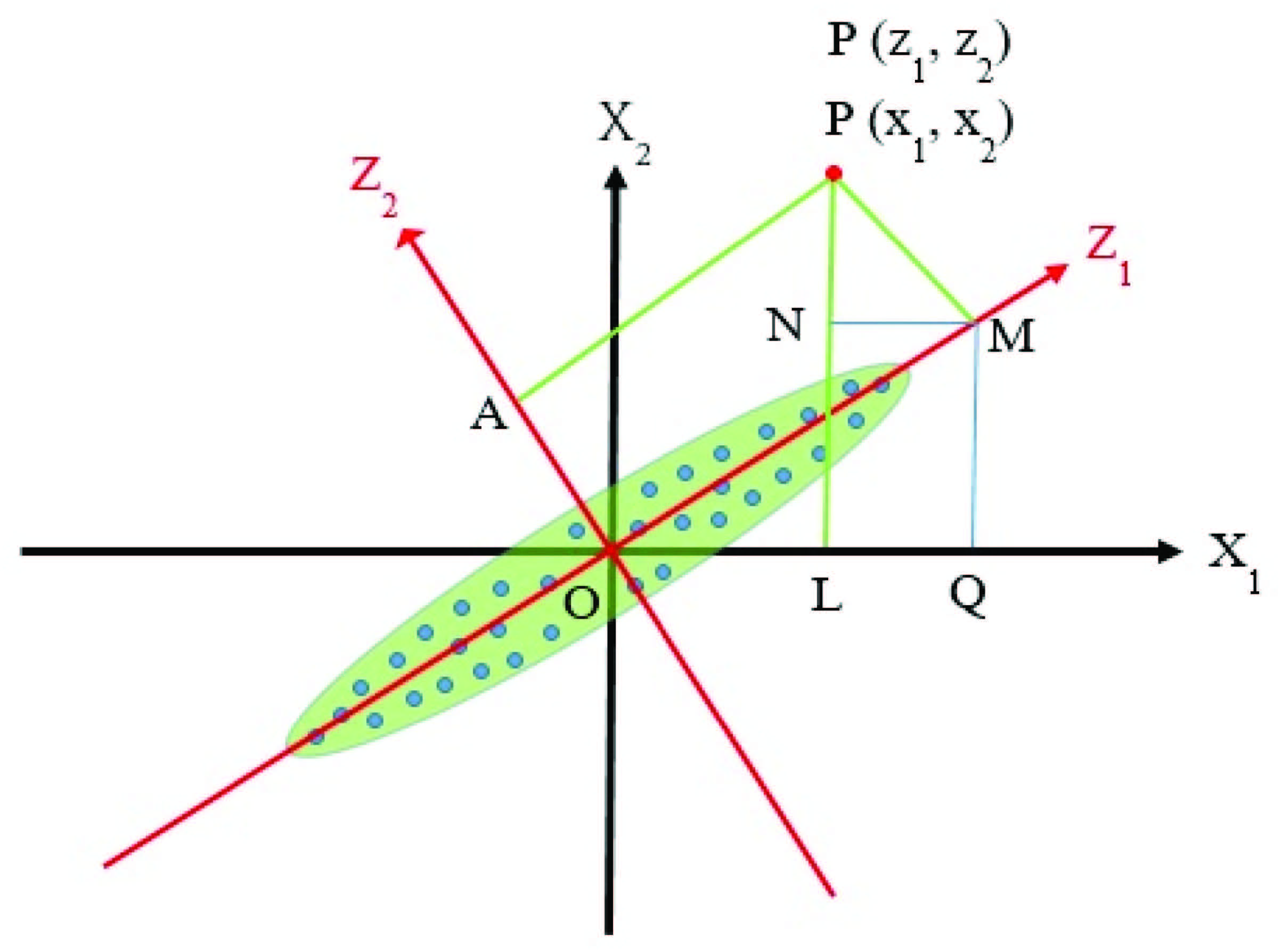
Figure 4 Coordinates of point P with respect to unrotated and rotated axes.

Now,

$\mathrm{OL}$	$=x_1\mathit{\hspace{1em}}\mathrm{PL}=x_2$
$\mathrm{OM}$	$=z_1\mathit{\hspace{1em}}\mathrm{PM}=z_2$

Again,

$\mathrm{OL}$	$=$	$\mathrm{OQ}-\mathrm{LQ}$	(15)
	$=$	$\mathrm{OQ}-\mathrm{MN}$
	$=$	$\mathrm{OM}\mathrm{COS}\mathrm{\theta }-\mathrm{PM}\mathrm{SIN}\mathrm{\theta }$
	$=$	$z_1\mathrm{COS}\mathrm{\theta }-z_2\mathrm{SIN}\mathrm{\theta }$

(From $\mathrm{\Delta }$OMQ and $\mathrm{\Delta }$PMN respectively)

and

$\mathrm{PL}$	$=$	$\mathrm{PN}+\mathrm{NL}$	(16)
	$=$	$\mathrm{PN}+\mathrm{MQ}$
	$=$	$\mathrm{PM}\mathrm{COS}\mathrm{\theta }+\mathrm{OM}\mathrm{SIN}\mathrm{\theta }$
	$=$	$z_2\mathrm{COS}\mathrm{\theta }+z_1\mathrm{SIN}\mathrm{\theta }$

(From $\mathrm{\Delta }$PMN and $\mathrm{\Delta }$OMQ respectively)

Solving Equation no. (15) and (16), it can be obtained,

$z_1$	$=x_1\mathrm{COS}\mathrm{\theta }+x_2\mathrm{SIN}\mathrm{\theta }$
$z_2$	$=x_2\mathrm{COS}\mathrm{\theta }-x_1\mathrm{SIN}\mathrm{\theta }$

In matrix form, which can be rewritten as (Aitken, 2016),

$\left[\begin{array}{c}\hfill z_1\hfill \\ \hfill z_2\hfill \end{array}\right]$

$=\left[\begin{array}{cc}\hfill COS\theta \hfill & \hfill SIN\theta \hfill \\ \hfill -SIN\theta \hfill & \hfill COS\theta \hfill \end{array}\right]\left[\begin{array}{c}\hfill x_1\hfill \\ \hfill x_2\hfill \end{array}\right]$

Or,

$$\overrightarrow{\mathrm{z}}=A^T\overrightarrow{x}$$

Or,

$$\overrightarrow{\mathrm{z}}=\left[\overrightarrow{a_1}\overrightarrow{a_2}\right]\overrightarrow{x}$$

Where,

$\overrightarrow{a_1}$	$=\left[\begin{array}{c}\hfill COS\theta \hfill \\ \hfill -SIN\theta \hfill \end{array}\right],{\overrightarrow{a}}_2=\left[\begin{array}{c}\hfill SIN\theta \hfill \\ \hfill COS\theta \hfill \end{array}\right]$
$\therefore \parallel {\overrightarrow{a}}_1\parallel$	$=1\mathit{\hspace{1em}\hspace{1em}}\mathrm{and}\mathit{\hspace{1em}\hspace{1em}}\parallel {\overrightarrow{a}}_2\parallel =1$

So, it can be observed that ${\overrightarrow{a}}_i$ ’s are unit vectors and $A^{T}A=I=A{A}^T$ i.e. transformation matrix A is an orthogonal matrix. Similarly, for n number of variables also, this can be generalised as,

$Z_j={\sum }_{i=1}^n{a}_{ji}{X}_i$, subjected to the condition $\overrightarrow{a}_j{}^T\overrightarrow{a_j}=1$.

As the ultimate objective of this transformation is to maximise the decrease of variance in such a manner that the last few number of variables can be easily chopped off, maximisation of $V(Z_j)$ is required subjected to the condition, $\overrightarrow{a}_j{}^T{\overrightarrow{a}}_j=1$.

Now,

$$V\left(Z_j\right)=\overrightarrow{a}_j{}^{T}S{\overrightarrow{a}}_j$$

here, S is the sample dispersion matrix of $X_1,X_2,\mathrm{\dots },X_n$ variables.

In other words, maximisation of $\overrightarrow{a}_j{}^{T}S{\overrightarrow{a}}_j$ is needed to be subjected to the condition,

$$\overrightarrow{a}_j{}^T{\overrightarrow{a}}_j-1=0.$$

Using Lagrangian multiplier, a function has been defined as,

$$L=\overrightarrow{a}_j{}^{T}S{\overrightarrow{a}}_j-\mathrm{\lambda }(\overrightarrow{a}_j{}^T{\overrightarrow{a}}_j-1)$$

Partially differentiating L with respect to $a_j$ and equating it to zero, it can be obtained,

$$\frac{\delta L}{\delta a_j}=0$$

Or,

$$2S{\overrightarrow{a}}_j-2\mathrm{\lambda }{\overrightarrow{a}}_j=0$$

Or,

$$\left(\mathrm{S}-\mathrm{\lambda }\mathrm{I}\right){\overrightarrow{a}}_j=0$$

(17)

Equation (17) is similar to the Equation (6) mentioned earlier, from which in the same fashion, the same results can be obtained,

(i) $\sum =\mathrm{\Delta }$,

(ii) $$\begin{array}{cc}\hfill {\sigma }_{ij}& ={\mathrm{\lambda }}_i,\mathrm{for}\mathit{\hspace{1em}}i=j\hfill \\ & =0,\mathrm{for}\hspace{1em}\hspace{0.25em}i\ne j,\hfill \end{array}$$

(iii) ${\sum }_{i=1}^n{\sigma }_{ij}={\sum }_{i=1}^n{\mathrm{\lambda }}_i$

and

(iv) proportion of variability explained by $i^{\mathrm{th}}$ $\mathrm{PC}=\frac{{\mathrm{\lambda }}_i}{{\sum }_{i=1}^n{\lambda }_i}$.

4 Conclusion

In this study, both algebraic and geometric basis of principal components have been discussed thoroughly, which may considerably help in understanding the inner constructs of principal components. From both the approaches, it has been found that eigen values and elements of the corresponding eigen vectors of sample dispersion matrix are the variances and the coefficients of the original variables, respectively, of the corresponding newly formed principal components.

References

Ahmed, N., Natarajan, T. and Rao, K.R. (1974). Discrete cosine transform, IEEE Transactions on Computers, 23(1), pp. 90–93.

Aitken, A.C. (2016). Determinants and Matrices, Brousson, Read BooksLtd.

Anderson, T.W. (2003). An Introduction to Multivariate Statistical Analysis (3${}^{\mathrm{rd}}$ Edition), New Jersey, John Wiley & Sons.

Bertsekas, D.P. (2014). Constrained Optimization and Lagrange Multiplier Methods, New York, Academic Press Inc.

Bunch, J.R. and Nielsen, C.P. (1978). Updating the singular value decomposition, Numerische Mathematik, 31(2), pp. 111–129.

Chatterjee, A. (2000). An introduction to the proper orthogonal decomposition, Current Science, 78(7), pp. 808–817.

Eisenhart, L.P. (2005). Coordinate Geometry, USA, Dover Publications Inc.

Gujarati, D.N., Porter, D.C. and Gunasekar, S. (2011). Basic Econometrics, New York, McGraw-Hill.

Hannachi, A., Jolliffe, I.T. and Stephenson, D.B. (2007). Empirical orthogonal functions and related techniques in atmospheric science: a review, International Journal of Climatology, 27, pp. 1119–1152.

Hardle, W.K. and Simar L. (2014). Applied Multivariate Statistical Analysis (4^th Edition), New York, Springer-Verlag New York, Inc.

Harris, R.J. (2001). A Primer of Multivariate Statistics (3${}^{\mathrm{rd}}$ Edition). Mahwah, Lawrence Erlbaum Associates, Inc., Publishers.

Hotelling, H. (1933). Analysis of a complex of statistical variables into principal components, Journal of Educational Psychology, 24,pp. 417–441.

Jackson, J.E. (1991). A User’s Guide to Principal Components, New Jersey, John Wiley & Sons, Inc.

Johnson, R.A. and Wichern, D.W. (2007). Applied Multivariate Statistical Analysis. Upper Saddle River, New Jersey, Pearson Education, Inc.

Johnson, R.M. (1963). On a theorem stated by Eckart and Young, Psychometrika, 28(3), pp. 259–263.

Johnstone, I.M. (2001). On the distribution of the largest eigenvalue in principal components analysis, The Annals of Statistics, 29(2),pp. 295–327.

Pearson, K. (1901). On lines and planes of closest fit to systems of points in space, Philosophical Magazines, 2, pp. 559–572.

Rencher, A.C. (2012). Methods of Multivariate Analysis (3${}^{\mathrm{rd}}$ Edition), New Jersey, John Wiley & Sons.

Riedel, T. and Sahoo, P.K. (1998). Mean Value Theorems and Functional Equations, Singapore, World Scientific Publishing Co. Pte. Ltd.

Searle, S.R. and Khuri, A.I. (2017). Matrix Algebra Useful for Statistics (2${}^{\mathrm{nd}}$ Edition), New Jersey, John Wiley & Sons, Inc.

Stark, H. and Yang, Y. (1998). Vector Space Projections: A Numerical Approach to Signal and Image Processing, Neural Nets, and optics, New York, John Wiley & Sons, Inc.

Timm, N.H. (2002). Applied Multivariate Analysis. New York, Springer-Verlag New York, Inc.

Zhang, F. (2011). Matrix Theory: Basic Results and Techniques (2^nd Edition), New York, Springer Science & Business Media.

Biographies

Pramit Pandit obtained his Bachelor’s degree (Hons.) in Agriculture from Uttar Banga Krishi Viswavidyalaya and Master’s (Ag.) majoring in Agricultural Statistics from University of Agricultural Sciences, Bengaluru. He was the recipient of ICAR-Junior Research Fellowship during his Master’s degree programme for securing All India basis 2nd rank in AIEEA-UG-2016 examination in Statistical Sciences. He also secured All India basis 1st rank in AICE-JRF/SRF(PGS)-2018 in Agricultural Statistics and qualified ICAR-NET-2018. He was awarded with the prestigious UAS Gold Medal 2019 along with the Professor G. Gurumurthy Memorial Gold Medal, Sri Godabanahal Thuppamma Basappa Mallikarjuna Gold Medal and Sri Nijalingappa’s 77th Birthday Commemoration Gold Medal for his exemplary academic excellence. He was also the recipient of best ‘Best M.Sc. Thesis Award’ for his research work on, ‘Statistical Models for Insect Count Data On Rice’, conducted under the supervision of Prof. K. N. Krishnamurthy.

K. N. Krishnamurthy received his B.Sc., M.Sc. and M.Phil. degrees in Statistics from Bangalore University and Ph.D. degree in Statistics from Himalayan University. Prof. Krishnamurthy is a recipient of the Best Teacher award from the National Institute for Education & Research, New Delhi during 2017. He is currently working as Head of the department as well as University Head of the Department of Agricultural Statistics, Applied Mathematics & Computer Science, University of Agricultural Sciences, GKVK, Bengaluru. He has 38 years of experience in teaching at the University.

K. B. Murthy received his B.Sc. and M.Sc. degrees in Mathematics from Mysore University and Ph.D. degree in Mathematics from Himalayan University. He has specialised in graph theory and applied sciences and has a teaching experience of over 25 years. He has published many papers in National and International Journals and also participated in many International conferences. He is a member of Board of Studies of University of Agricultural Sciences, GKVK, Bengaluru. Dr. K. B. Murthy is the recipient of the GAURAVACHARYA-2017 award for the significant contribution in the field of graph theory and education from National Institute for Education and Research, New Delhi.

Journal of Reliability and Statistical Studies, Vol. 13_1, 73–86.
doi: 10.13052/jrss0974-8024.1314
© 2020 River Publishers

Abstract

1 Introduction

2 Algebraic Basis of Principal Components

3 Geometric Basis of Principal Component

4 Conclusion

References

Biographies