The Marshall-Olkin Modified Lindley Distribution: Properties and Applications

Jiju Gillariose^1,*, Lishamol Tomy², Farrukh Jamal³ and Christophe Chesneau⁴

¹Department of Statistics, St.Thomas College, Pala, Kerala, India

²Department of Statistics, Deva Matha College, Kuravilangad, Kerala, India

³Department of Statistics, The Islamia University, Bahawalpur 63100, Pakistan

⁴Université de Caen, LMNO, Campus II, Science 3, Caen, 14032, France

E-mail: jijugillariose@yahoo.com; lishatomy@gmail.com; drfarrukh1982@gmail.com; christophe.chesneau@unicaen.fr

Corresponding Author

Received 16 November 2019; Accepted 20 June 2020; Publication 28 October 2020

Abstract

This article is devoted to a new Marshall-Olkin distribution by using a recent modification of the Lindley distribution. Mathematical features of the new model are described. Utilizing maximum likelihood method, the parameters of the new model are estimated. Performance of the estimation approach is discussed by means of a simulation procedure. Moreover, applications of the new distribution are presented which reveal its superiority over other three competing Marshall-Olkin extended distributions of the literature.

Keywords: Data analysis; marshall-olkin generalization; modified lindley distribution.

1 Background

The Lindley distribution (Lindley 1958, 1965) has pointed out various statisticians to construct new distributions due to its desirable properties. In the past few decades, numerous research papers dealing with this distribution have subsequently appeared in the statistics literature, for instance, Ghitany et al. (2008), Krishna and Kumar (2011), Deniz and Ojeda (2011), Al-Mutairi et al. (2013), Shanker et al. (2015), and Sharma et al. (2015). Moreover, wide varieties of Lindley distributions was also derived and studied, such as, generalized Poisson-Lindley by Mahmoudi and Zakerzadeh (2010), quasi Lindley distribution by Shanker and Mishra (2013), transmuted Lindley distribution by Merovci (2013), transmuted Lindley-geometric distribution by Merovci and Elbatal (2014), beta-Lindley distribution by Merovci and Sharma (2014), Harris extended two-parameter Lindley distribution by Tomy et al. (2019) and discrete Harris extended Lindley distribution by Thomas et al. (2019). Tomy (2018) provides a comprehensive review study on the Lindley distribution.

More recently, a new modified Lindley (ML) distribution has been proposed by Chesneau et al. (2019a). According to Chesneau et al. (2019a) “the survival function (sf) and probability density function (pdf) of the ML distribution are defined by

$$\overline{F}(x,\theta )=\left[1+\frac{\theta x}{1+\theta }{e}^{-\theta x}\right]e^{-\theta x};x,\theta >0$$

(1)

and

$$f(x,\theta )=\frac{\theta }{1+\theta }{e}^{-2\theta x}\left[(1+\theta )e^{\theta x}+2\theta x-1\right];x,\theta >0,$$

(2)

respectively”. An eminent feature of the ML model is that $f(x,\theta )$ can be represented as a weighted sum of exponential and gamma pdfs. It also reveals to be an intermediary distribution between the exponential and former Lindley distribution, in the first stochastic ordering sense. Recently, two extensions for the ML distribution such as the inverse ML (see, Chesneau et al., 2020) and the wrapped ML (see, Chesneau et al., 2019b) distributions have been proposed.

In addition, the statistical distribution theory involves many flexible models which have been built using the Marshall-Olkin extended (MOE) scheme introduced by Marshall and Olkin (1997). The resulting new models are known to give more versatility to model numerous types of data sets. The early researches employing this technique by Lam and Leung (2001), Economou and Caroni (2007), Rao et al. (2009), Nanda and Das (2012), Rubio and Steel (2012), Cordeiro et al. (2014) and Castellares and Lemonte (2016). According to Marshall and Olkin (1997), “the sf and pdf of the MOE class are defined, by

$$\overline{G}(x,\gamma )=\frac{\gamma \overline{F}(x)}{1-\overline{\gamma }\overline{F}(x)};x\in ℝ,\gamma >0,\overline{\gamma }=1-\gamma$$

(3)

and

$$g(x,\gamma )=\frac{\gamma f(x)}{{[1-\overline{\gamma }\overline{F}(x)]}^2};x\in ℝ,\gamma >0,$$

(4)

respectively. The corresponding hazard rate function (hrf) is defined by

$$h(x,\gamma )=\frac{r(x)}{1-\overline{\gamma }\overline{F}(x)}$$

where $f(x)$ and $r(x)$ are the pdf and hrf corresponding to the sf of the baseline distribution $\overline{F}(x)$, respectively.”

In this work, we explore an extension of the ML model through the MOE approach. The main interest for pioneering the new model is that it is an extended form providing various features. Also, its pdf and hrf are quite simple. The proposed model has only two parameters. Further, the grandness of the proposed model lies in its skill to fit different real data sets. Thus, we introduce this distribution with hope that the related model may provide better fit in certain practical contexts than other Marshall-Olkin models.

The outline of the paper is described as follows. The relevant statistical functions associated with the proposed distribution are stated Section 2. The statistical properties are inspected in Section 3. Maximum likelihood estimation of the unknown parameters is presented in Section 4, completed by a simulation procedure. Utilizations of the newly developed model is discussed in Section 5. Eventually, summary is addressed in Section 6.

2 MOE Modified Lindley Distribution

Motivated by the advantages of ML distribution, we propose a new distribution, namely, MOE Modified Lindley (MOEML) distribution. By using two Equations (1) and (3), the sf of the MOEML model is given by

$$\overline{G}(x,\gamma ,\theta )=\frac{\gamma \left(1+\frac{\theta x}{1+\theta }{e}^{-\theta x}\right)e^{-\theta x}}{1-\overline{\gamma }\left(1+\frac{\theta x}{1+\theta }{e}^{-\theta x}\right)e^{-\theta x}};x,\theta ;\gamma >0$$

(5)

Also, the pdf of the MOEML distribution is

$$g(x,\gamma ,\theta )=\frac{\gamma \theta e^{-2\theta x}\left[(1+\theta )e^{\theta x}+2\theta x-1\right]}{(1+\theta ){\left[1-\overline{\gamma }\left(1+\frac{\theta x}{1+\theta }{e}^{-\theta x}\right)e^{-\theta x}\right]}^2};x,\theta ,\gamma >0$$

(6)

Remark that, for $\gamma =1$, we obtain the ML distribution. In addition, the hrf of the MOEML distribution becomes

$$h(x,\gamma ,\theta )=\frac{\theta (\theta x-1)+\theta (1+\theta )e^{\theta x}+{\theta }^{2}x}{\left[1-\overline{\gamma }\left(1+\frac{\theta x}{1+\theta }{e}^{-\theta x}\right)e^{-\theta x}\right][(1+\theta )e^{\theta x}+\theta x]};x,\theta ,\gamma >0$$

(7)

Figure 1 Pdf curves of the MOEML model.

Also, cumulative hazard rate function of MOEML distribution is

$H(x,\gamma ,\theta )$	$=-\log [\overline{G}(x,\gamma ,\theta )]$
	$=-\log (\gamma )-\log \left(1+{\displaystyle \frac{\theta x}{1+\theta }}{e}^{-\theta x}\right)+\theta x$
	$+\log \left[1-\overline{\gamma }\left(1+{\displaystyle \frac{\theta x}{1+\theta }}{e}^{-\theta x}\right)e^{-\theta x}\right]$

The corresponding quantile function, is denoted as $Q(u,\gamma ,\theta )$, can be determined by solving the equation: $G[Q(u,\gamma ,\theta ),\gamma ,\theta ]=Q[G(u,\gamma ,\theta ),\gamma ,\theta ]=u,u\in (0,1)$. It can not be presented analytically but can be calculated numerically. The structures of pdf and hrf for selected parameters of $\gamma$ and $\theta$ are shown in Figures 1 and 2, respectively. From the plots, we also remark that the pdf has right skewed, left skewed, (more or less) symmetrical and reverse J shapes. Further, the plot also shows MOEML hrf can be decreasing, increasing, constant and upside down bathtub shape.

Figure 2 Hrf curves of the MOEML model.

3 General Properties

3.1 Useful Expansions

In this subsection, general properties of the MOEML are derived and discussed. We now give pdf expansions of the MOEML distribution. The distribution of generalized binomial formula ensuring that

$${(1-z)}^{-r}={\sum }_{i=0}^{\mathrm{\infty }}\left(\begin{array}{c}r+i-1\hfill \\ i\hfill \end{array}\right)z^i,|z|<1,r>0$$

(8)

Now, we must distinguish two cases. If $0<\gamma <1$, then $1-\gamma \in (0,1)$, hence using expansion (8) in (6), we get the representation for the pdf of MOEML distribution as

$$g(x,\gamma ,\theta )={\sum }_{j=0}^{\mathrm{\infty }}{\sum }_{k=0}^j{\omega }_{j,k}{x}^k\left[(1+\theta )e^{\theta x}+2\theta x-1\right]e^{-(2+k+j)\theta x}$$

(9)

where

$${\omega }_{j,k}=\frac{(j+1)\left(\begin{array}{c}j\hfill \\ k\hfill \end{array}\right){\overline{\gamma }}^j\gamma {\theta }^{k+1}}{{(1+\theta )}^{k+1}}$$

If $\gamma >1$, then $\overline{\gamma }/\gamma \in (0,1)$, so we have

$$[1-\overline{\gamma }(1-S)]=\gamma \left[1+\frac{\overline{\gamma }}{\gamma }S\right]$$

(10)

where $S=1-\overline{F}(x,\theta )$. Thus, from (10) and (6) the pdf of MOEML as

$$g(x,\gamma ,\theta )={\sum }_{i=0}^{\mathrm{\infty }}{\sum }_{j=0}^i{\sum }_{k=0}^{\mathrm{\infty }}{\omega }_{i,j,k}^{*}{x}^k\left[(1+\theta )e^{\theta x}+2\theta x-1\right]e^{-(2+k+j)\theta x}$$

(11)

where

$${\omega }_{i,j,k}^{*}=\frac{{(-1)}^{i+j}(i+1)\left(\begin{array}{c}i\hfill \\ j\hfill \end{array}\right)\left(\begin{array}{c}j\hfill \\ k\hfill \end{array}\right){\overline{\gamma }}^i{\theta }^{k+1}}{{\gamma }^{i+1}{(1+\theta )}^{k+1}}$$

3.2 Moments and Related Quantities

Let X denote a random variable adopting the MOEML model.

Now, we know

$${\mu }_r^{{}^{\prime }}=E(X^r)={\int }_0^{\mathrm{\infty }}{x}^{r}g(x,\gamma ,\theta )𝑑x$$

Hence, the $r^{th}$ moment of MOEML distribution, when $0<\gamma <1$ is given by

${\mu }_r^{{}^{\prime }}$	$={\displaystyle \sum _{j=0}^{\mathrm{\infty }}}{\displaystyle \sum _{k=0}^j}{\omega }_{j,k}{\displaystyle {\int }_0^{\mathrm{\infty }}}{x}^{k+r}\left[(1+\theta )e^{\theta x}+2\theta x-1\right]e^{-(2+k+j)\theta x}𝑑x$
	$={\displaystyle {\sum }_{j=0}^{\mathrm{\infty }}}{\displaystyle {\sum }_{k=0}^j}{\omega }_{j,k}\mathrm{\Gamma }(r+k+1){\varrho }_{k,j}$

where

$${\varrho }_{k,j}=\left\{\frac{\theta +1}{{[\theta (1+j+k)]}^{r+k+1}}+\frac{2\theta (r+k+1)}{{[\theta (2+j+k)]}^{r+k+1}}-\frac{1}{{[\theta (2+j+k)]}^{r+k+1}}\right\}$$

Similarly, when $\gamma >1$

$${\mu }_r^{{}^{\prime }}=\sum _{i=0}^{\mathrm{\infty }}\sum _{j=0}^i\sum _{k=0}^{\mathrm{\infty }}{\omega }_{i,j,k}^{*}\mathrm{\Gamma }(r+k+1){\varrho }_{k,j}$$

where $\mathrm{\Gamma }(r+k+1)=(r+k)!$. We can calculate $r^{th}$ moments by using the above expressions, for $0<\gamma <1$ and $\gamma >1$, respectively. Table 1 presents the first four moments, $\sqrt{{\beta }_1}=\sqrt{{\mu }_3^2/{\mu }_2^3}$ and ${\beta }_2={\mu }_4/{\mu }_2^2$, where ${\mu }_r$ denotes the $r^{th}$ central moment of X, of the MOEML model for adopted values of $\gamma \mathrm{and}\theta$.

Table 1 Some characteristics of the of the MOEML distribution

	$(\gamma ,\theta )$	$(\gamma ,\theta )$	$(\gamma ,\theta )$	$(\gamma ,\theta )$	$(\gamma ,\theta )$	$(\gamma ,\theta )$
	(5,5)	(5,0.5)	(0.5,5)	(0.5,0.5)	(2,2)	(10,10)
${\mu }_1^{{}^{\prime }}$	0.4100	4.3133	0.1461	1.7021	0.7352	9.1095
${\mu }_2^{{}^{\prime }}$	0.0737	6.9557	0.0277	2.7693	0.3337	123.4979
${\mu }_3^{{}^{\prime }}$	0.0214	19.6496	0.0115	10.6231	0.2863	4310.76
${\mu }_4^{{}^{\prime }}$	0.0266	243.8674	0.0096	88.7936	0.72431	273038.1
$\sqrt{{\beta }_1}$	1.0722	1.07112	2.5002	2.3052	1.4852	3.1410
${\beta }_2$	4.8963	5.04042	12.5791	11.5784	6.5045	17.9021

From Table 1, we see that the MOEML distribution can be slightly or highly right skewed. Also, it can be (near) mesokurtic and leptokurtic. Let us now introduce the $r^{\mathrm{th}}$ incomplete moment of $X$. For $x>0$, it is given by

$${\mu }_r^{*}(x)={\int }_0^x{t}^{r}g(t,\gamma ,\theta )𝑑t$$

Also, the incomplete mean (that is, when $r=1$ and $0<\gamma <1$) is expressed by:

${\mu }_1^{*}(x)$	$=$	${\displaystyle \sum _{j=0}^{\mathrm{\infty }}}{\displaystyle \sum _{k=0}^j}{\omega }_{j,k}\left[{\displaystyle {\int }_0^x}{t}^{k+1}[(1+\theta )e^{\theta t}+2\theta t-1]e^{-(2+k+j)\theta t}𝑑t\right]$	(12)
	$=$	${\displaystyle \sum _{j=0}^{\mathrm{\infty }}}{\displaystyle \sum _{k=0}^j}{\omega }_{j,k}[(1+\theta ){\displaystyle {\int }_0^x}{t}^{k+1}{e}^{-(1+k+j)\theta t}dt$
		$+2\theta {\displaystyle {\int }_0^x}{t}^{k+2}{e}^{-(2+k+j)\theta t}dt-{\displaystyle {\int }_0^x}{t}^{k+1}{e}^{-(2+k+j)\theta t}dt]$
	$=$	${\displaystyle {\sum }_{j=0}^{\mathrm{\infty }}}{\displaystyle {\sum }_{k=0}^j}{\omega }_{j,k}{\varrho }_{k,j}^{*}$

where

${\varrho }_{k,j}^{*}$	$=[(1+\theta ){\displaystyle \frac{\gamma (k+2,(1+k+j)\theta x)}{{[(1+k+j)\theta ]}^{k+2}}}+2\theta {\displaystyle \frac{\gamma (k+3,(2+k+j)\theta x)}{{[(2+k+j)\theta ]}^{k+3}}}$
	$-{\displaystyle \frac{\gamma (k+2,(2+k+j)\theta x)}{{[(2+k+j)\theta ]}^{k+2}}}]$

and $\gamma (a,x)={\int }_0^x{t}^{a-1}{e}^{-t}𝑑t$ is the incomplete gamma function.

Also, the incomplete mean, when $\gamma >1$ is given by:

$${\mu }_1^{*}(x)={\sum }_{i=0}^{\mathrm{\infty }}{\sum }_{j=0}^i{\sum }_{k=0}^{\mathrm{\infty }}{\omega }_{j,k}^{*}{\varrho }_{k,j}^{*}$$

(13)

Moment generating function is given by the following formula

$$M_X(t)=E(e^{tX})={\sum }_{r=0}^{\mathrm{\infty }}\frac{t^r}{r!}E(X^r)$$

When $0<\gamma <1$, it has following form

$$M_X(t)=\sum _{j=0}^{\mathrm{\infty }}\sum _{k=0}^j\sum _{r=0}^8\frac{{\omega }_{j,k}{t}^r\mathrm{\Gamma }(r+k+1)}{r!}{\varrho }_{k,j}$$

Similarly, when $\gamma >1$

$$M_X(t)=\sum _{i=0}^{\mathrm{\infty }}\sum _{j=0}^i\sum _{k=0}^{\mathrm{\infty }}\sum _{r=0}^{\mathrm{\infty }}\frac{{\omega }_{i,j,k}^{*}\mathrm{\Gamma }(r+k+1)t^r}{r!}{\varrho }_{k,j}$$

3.3 Mean Deviation (MD), Bonferroni and Lorenz Curves

First of all, the MD (about the mean, denoted by $\mu$) is defined by

$$MD={\int }_0^{\mathrm{\infty }}|x-\mu |g(x,\gamma ,\theta )𝑑x$$

which can be obtained as

$$MD=2\mu G(\mu ,\gamma ,\theta )-2{\mu }_1^{*}(\mu )$$

where ${\mu }_1^{*}(\mu )$ denotes the incomplete mean already expressed in (12) or (13), depending on the value of $\gamma$, taken with $x=\mu .$

The graph of $B\left[G(x,\gamma ,\theta )\right]$ across $x$ is called Bonferroni curve, where

$$B[G(x,\gamma ,\theta )]=\frac{1}{{\mu }_{1}G(x,\gamma ,\theta )}{\mu }_1^{*}(x)$$

The plot of $L[G(x,\gamma ,\theta )]$ across $x$ is Lorenz curve, where $L[G(x,\gamma ,\theta )]=G(x,\gamma ,\theta )B[G(x,\gamma ,\theta )]$. In economics, both curves play very critical role in studying income and poverty.

4 Estimation Method with Simulation

4.1 Estimation Method

Consider $x_1,x_2,\mathrm{\dots },x_n$ be $n$ independent observations from the MOEML model. For determining the maximum likelihood estimates (MLEs) of $\gamma$ and $\theta$, we have following likelihood function

$L(\theta ,\gamma )$	$={\displaystyle \prod _{i=1}^n}g(x_i,\gamma ,\theta )$
	$={\displaystyle \frac{{\gamma }^n{\theta }^n}{{(1+\theta )}^n}}{e}^{-2\theta {\sum }_{i=1}^n{x}_i}{\displaystyle \prod _{i=1}^n}{\displaystyle \frac{\left[(1+\theta )e^{\theta x_i}+2\theta x_i-1\right]}{{\left[1-\overline{\gamma }\left(1+\frac{\theta x_i}{1+\theta }{e}^{-\theta x_i}\right)e^{-\theta x_i}\right]}^2}}$

Then, the log-likelihood function is specified as

$L(\theta ,\gamma )$	$=n\log (\gamma \theta )-n\log (1+\theta )-2\theta {\displaystyle \sum _{i=1}^n}{x}_i+{\displaystyle \sum _{i=1}^n}\log \left[(1+\theta )e^{\theta x_i}+2\theta x_i-1\right]$
	$-2{\displaystyle \sum _{i=1}^n}\log \left[1-\overline{\gamma }\left(1+{\displaystyle \frac{\theta x_i}{1+\theta }}{e}^{-\theta x_i}\right)e^{-\theta x_i}\right]$

The MLE for $\theta$ and $\gamma$ are accessed by solving $\partial L(\theta ,\gamma )/\partial \theta =0$ and $\partial L(\theta ,\gamma )/\partial \gamma =0$, that is,

	${\displaystyle \frac{n}{\theta }}-{\displaystyle \frac{n}{1+\theta }}-2{\displaystyle \sum _{i=1}^n}{x}_i+{\displaystyle \sum _{i=1}^n}{\displaystyle \frac{e^{\theta x_i}(\theta x_i+x_i+1)+2x_i}{(1+\theta )e^{\theta x_i}+2\theta x_i-1}}$
	$+2{\displaystyle \sum _{i=1}^n}{\displaystyle \frac{\gamma x_i{e}^{-\theta x_i}\left[x_i+2x_i^2\theta \frac{e^{-\theta x_i}}{1+\theta }+\frac{e^{-\theta x_i}}{{(1+\theta )}^2}\right]}{\left[1-\overline{\gamma }\left(1+\frac{\theta x_i}{1+\theta }{e}^{-\theta x_i}\right)e^{-\theta x_i}\right]}}=0$

and

$$\frac{n}{\gamma }-2{\sum }_{i=1}^n\frac{\left(1+\frac{\theta x_i}{1+\theta }{e}^{-\theta x_i}\right)e^{-\theta x_i}}{\left[1-\overline{\gamma }\left(1+\frac{\theta x_i}{1+\theta }{e}^{-\theta x_i}\right)e^{-\theta x_i}\right]}=0$$

There is no analytical solution for these equations, but the MLEs can be determined at least numerically with any mathematical software.

4.2 Simulation

In this subsection, the behaviors of the considered MLEs of model parameters are now compared based on randomly generated $N=3000$ samples of values of different sizes following the inverse transform sampling algorithm. In this regard, we investigate their (average) Bias and mean square error (MSE) defined as follows:

$$\mathrm{M}LE(n)=\frac{1}{N}\sum _{i=1}^N{\widehat{\delta }}_i,\mathrm{B}ias(n)=\mathrm{M}LE(n)-\delta ,\mathrm{M}SE(n)=\frac{1}{N}\sum _{i=1}^N{({\widehat{\delta }}_i-\delta )}^2,$$

where $\delta \in \{\theta ,\gamma \}$ and ${\widehat{\delta }}_i$ denotes the obtained MLE at the $i$-th sample.

Figures 3, 5, 7 and 9 present graphically the evolution of the Bias for the estimates for $n$ from 10 to 50 for selected values of $\theta$ and $\gamma$. Also, Figures 4, 6, 8 and 10 present graphically the evolution of the MSE for the estimates for $n$ from 10 to 50 for the same selected values of $\theta$ and $\gamma$.

We can see that all the curves representing the Bias and MSE tend quickly to 0 when n increases, showing the efficiency of the method.

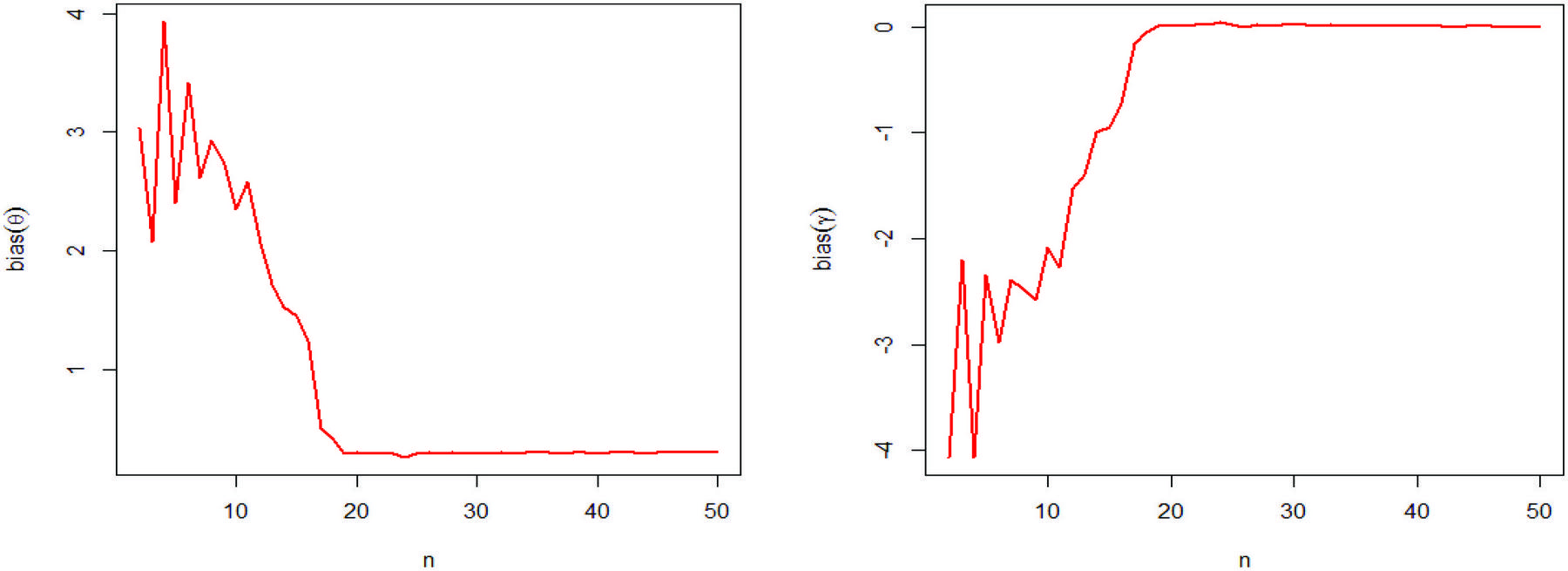
Figure 3 Figures of the Bias of MLE for $\theta =0.5$ and $\gamma =3.$

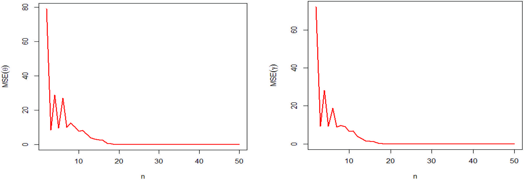
Figure 4 Figures of the MSE of MLE for $\theta =0.5$ and $\gamma =3$.

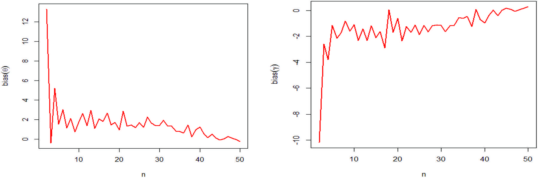
Figure 5 Figures of the Bias of MLE for $\theta =2$ and $\gamma =3$.

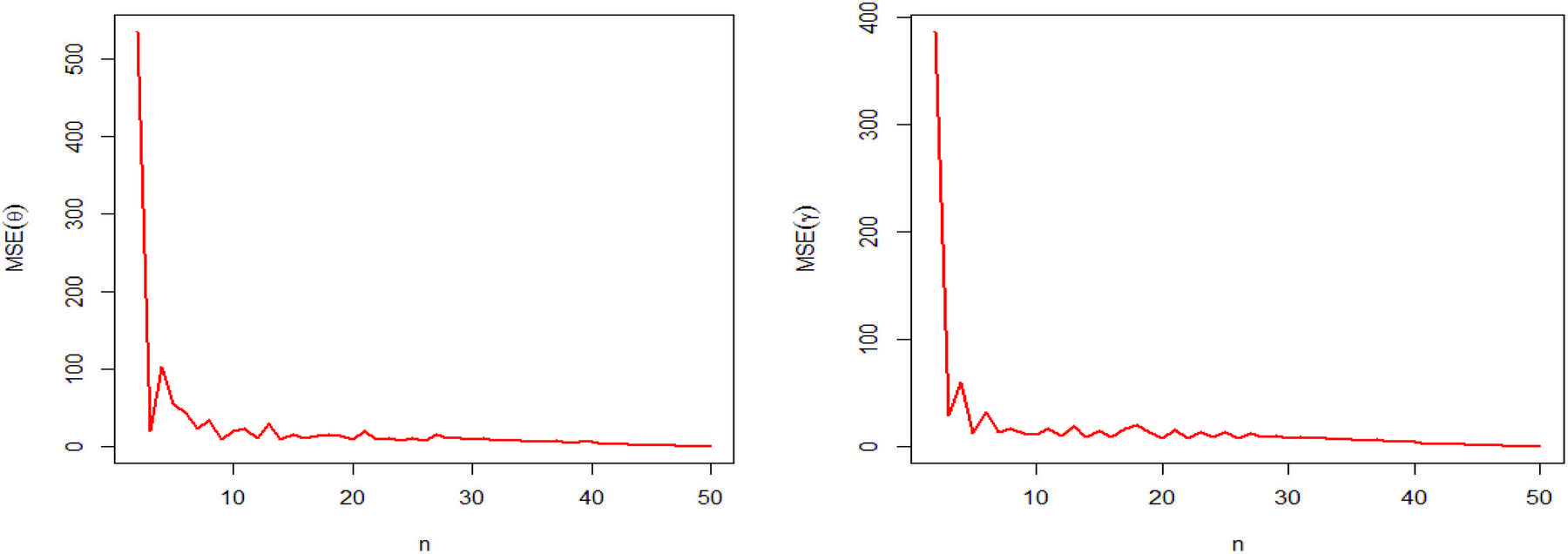
Figure 6 Figures of the MSE of MLE for $\theta =2$ and $\gamma =3$.

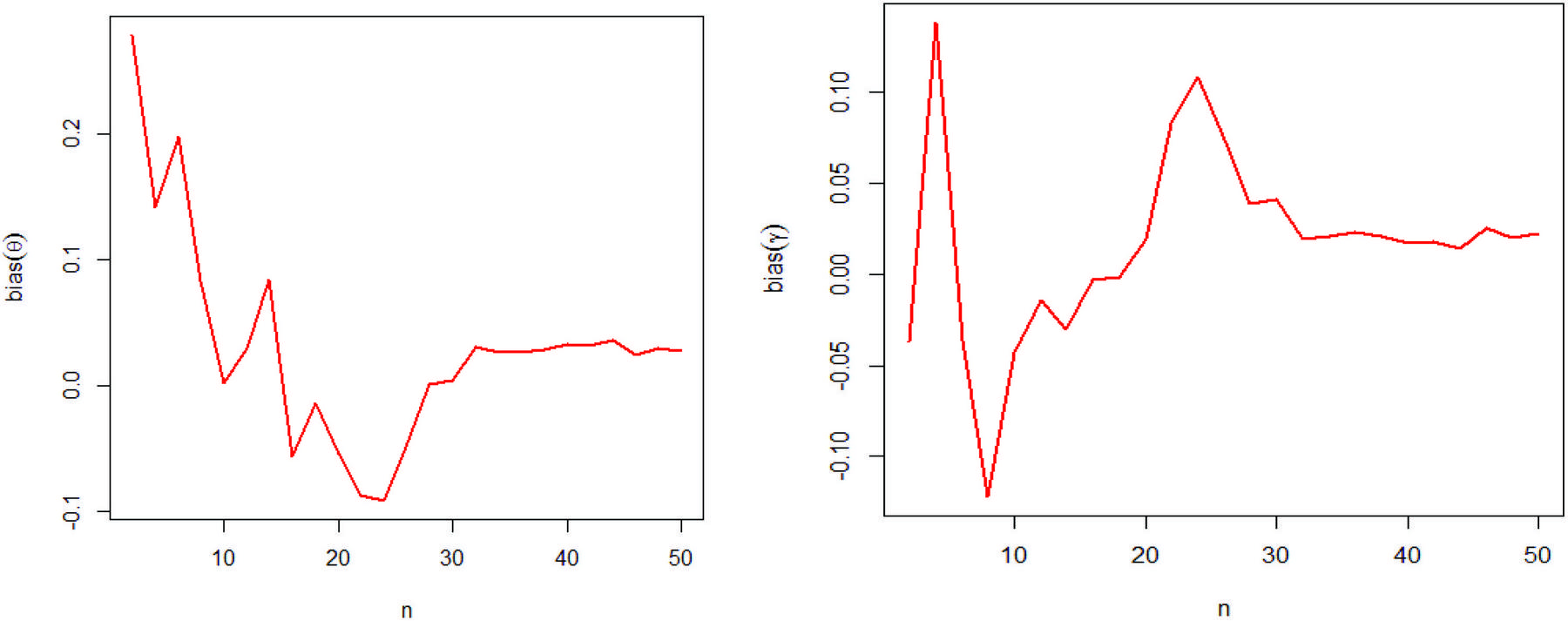
Figure 7 Figures of the Bias of MLE for $\theta =0.5$ and $\gamma =0.5$.

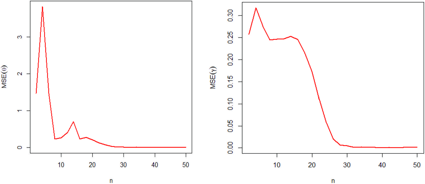
Figure 8 Figures of the MSE of MLE for $\theta =0.5$ and $\gamma =0.5$.

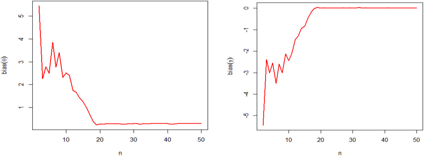
Figure 9 Figures of the Bias of MLE for $\theta =3$ and $\gamma =0.5$.

Figure 10 Figures of the MSE of MLE for $\theta =3$ and $\gamma =0.5$

5 Applications

The versatility of the MOEML model is engraved by exercising two practical datasets. We compare the fitting ability of the MOEML model with another MOE distributions, such as, MOE Exponential (MOEE) (Marshall and Olkin, 1997), MOE Frechet (MOEF) (Krishna et al., 2013) and MOE Lomax (MOEL) distributions (Ghitany et al., 2007). For comparing the usefulness of the models, we estimated the unknown parameters, standard error (SE), $-$log likelihood ($-$logL), the values of the AIC (Akaike Information Criterion) and BIC (Bayesian Information Criterion), AICc (corrected AIC), Kolmogorov-Smirnov (K-S) statistic (with $p$-values).

Dataset I depicts the fatigue life of some aluminum coupons cut in specific manner (see, Birnbaum and Saunders, 1969). The dataset (after subtracting 65) is:

Dataset I: 5, 25, 31, 32 ,34 ,35 ,38, 39, 39, 40, 42, 43, 43, 43, 44, 44, 47, 47, 48, 49, 49, 49, 51, 54, 55, 55, 55, 56, 56, 56, 58, 59, 59, 59, 59, 59, 63, 63, 64, 64, 65, 65, 65, 66, 66, 66, 66, 66, 67, 67, 67, 68, 69, 69, 69, 69, 71, 71, 72, 73, 73, 73, 74, 74, 76, 76, 77, 77, 77, 77, 77, 77, 79, 79, 80, 81, 83, 83, 84, 86, 86, 87, 90, 91, 92, 92, 92, 92, 93, 94, 97, 98, 98, 99, 101, 103, 105, 109, 136, 147.

The second data set representing the amount of cycles up to remissness of the yarn have been given by Picciotto (1970). The data set is:

Dataset II: 86, 146, 251, 653, 98, 249, 400, 292, 131, 169, 175, 176, 76, 264, 15, 364, 195, 262, 88, 264, 157, 220, 42, 321 ,180, 198, 38, 20, 61, 121, 282, 224, 149, 180, 325, 250, 196, 90, 229, 166, 38, 337, 65, 151, 341, 40, 40, 135, 597, 246, 211, 180, 93, 315, 353, 571, 124, 279, 81, 186, 497, 182, 423, 185, 229, 400, 338, 290, 398, 71, 246, 185, 188, 568, 55, 55, 61, 244, 20, 284, 393, 396, 203, 829, 239, 236, 286, 194, 277, 143, 198, 264, 105, 203, 124, 137, 135, 350, 193, 188.

Table 2 Comparison criterion for Dataset I

Distribution	Estimates(SE)	$-$logL	AIC	BIC	AICc	K-S statistic	$p$-value
MOEML	$\widehat{𝜽}\mathbf{=}\mathbf{0.0777}\mathbf{(}\mathbf{0.0074}\mathbf{)}$	450.3713	904.7427	909.953	904.8664	0.0478	0.9764
	$\widehat{𝜸}\mathbf{=}\mathbf{186.5067}\mathbf{(}\mathbf{101.92}\mathbf{)}$
MOEE	$\widehat{\alpha }=140.2547(59.2112)$	450.821	905.6421	910.8524	905.7658	0.0612	0.8473
	$\widehat{\theta }=0.0736(0.0059)$
MOEF	$\widehat{\alpha }=280.397(115.6240)$	475.1469	956.2938	964.1093	956.5438	0.1533	0.0181
	$\widehat{\eta }=3.1129(0.1753)$
	$\widehat{\beta }=10.3298(0.9250)$
MOEL	$\widehat{\alpha }=6.3887(12.822)$	461.2333	928.4665	936.2821	928.7165	0.1470	0.0266
	$\widehat{\theta }=0.0049(6.906e^{-04})$
	$\widehat{\beta }=4.3510(1.7832)$

Table 3 Comparison criterion for Dataset II

Distribution	Estimates(SE)	$-$logL	AIC	BIC	AICc	K-S statistic	$p$-value
MOEML	$\widehat{𝜽}\mathbf{=}\mathbf{0.0087}\mathbf{(}\mathbf{0.0013}\mathbf{)}$	624.1386	1252.277	1257.488	1252.4007	0.0694	0.7215
	$\widehat{𝜸}\mathbf{=}\mathbf{3.2305}\mathbf{(}\mathbf{1.3951}\mathbf{)}$
MOEE	$\widehat{\alpha }=6.5513(2.1169)$	625.1886	1254.377	1259.587	1254.50	0.0703	0.7062
	$\widehat{\theta }=0.0102(0.0012)$
MOEF	$\widehat{\alpha }=120.9476(75.5539)$	630.2481	1266.4960	1274.3120	1266.746	0.1533	0.0181
	$\widehat{\eta }=2.2599(0.1801)$
	$\widehat{\beta }=22.0462(5.1362)$
MOEL	$\widehat{\alpha }=38.5549(18.9074)$	625.2696	1256.539	1264.355	1256.789	0.0812	0.5255
	$\widehat{\theta }=0.0079(0.0023)$
	$\widehat{\beta }=3.9655(0.5590)$

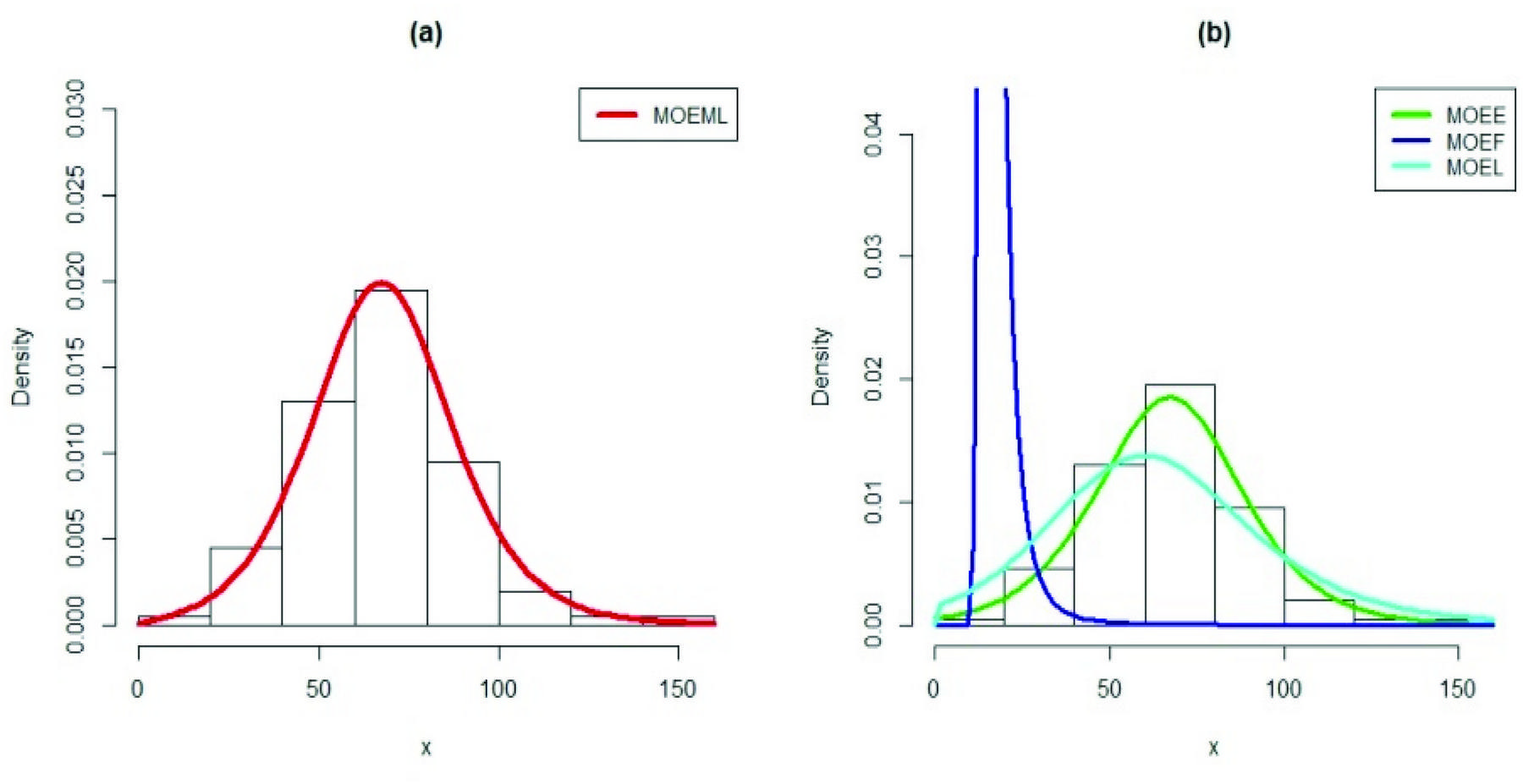
Figure 11 Fitted pdf plots for Dataset I.

Figure 12 Fitted pdf plots for Dataset II.

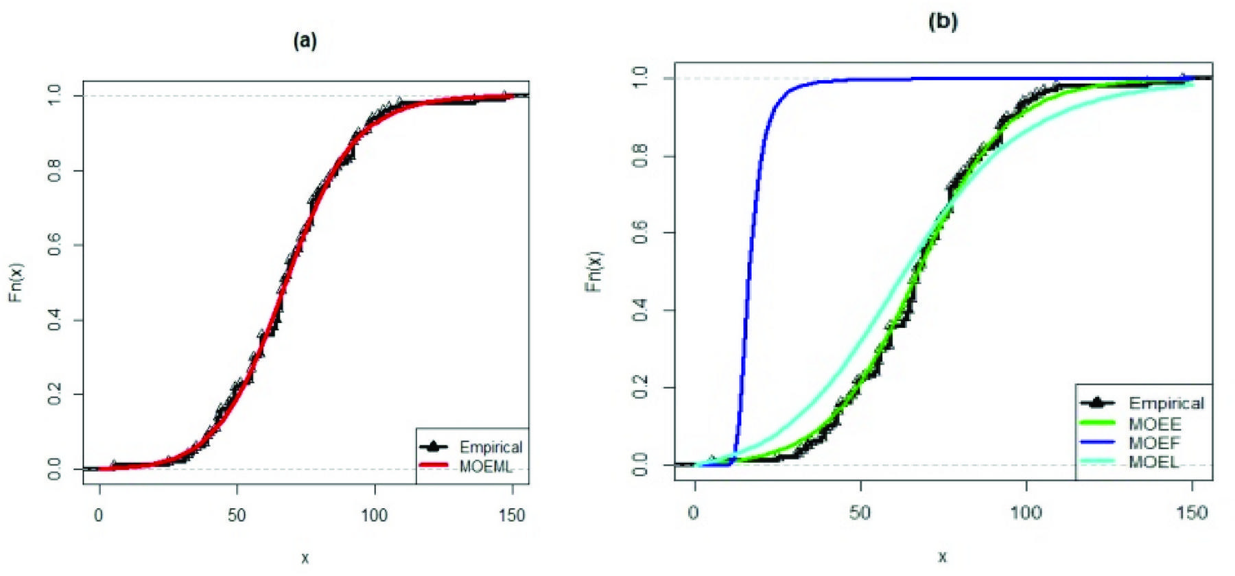
Figure 13 Fitted cdf plots for Dataset I.

Figure 14 Fitted cdf plots for Dataset II.

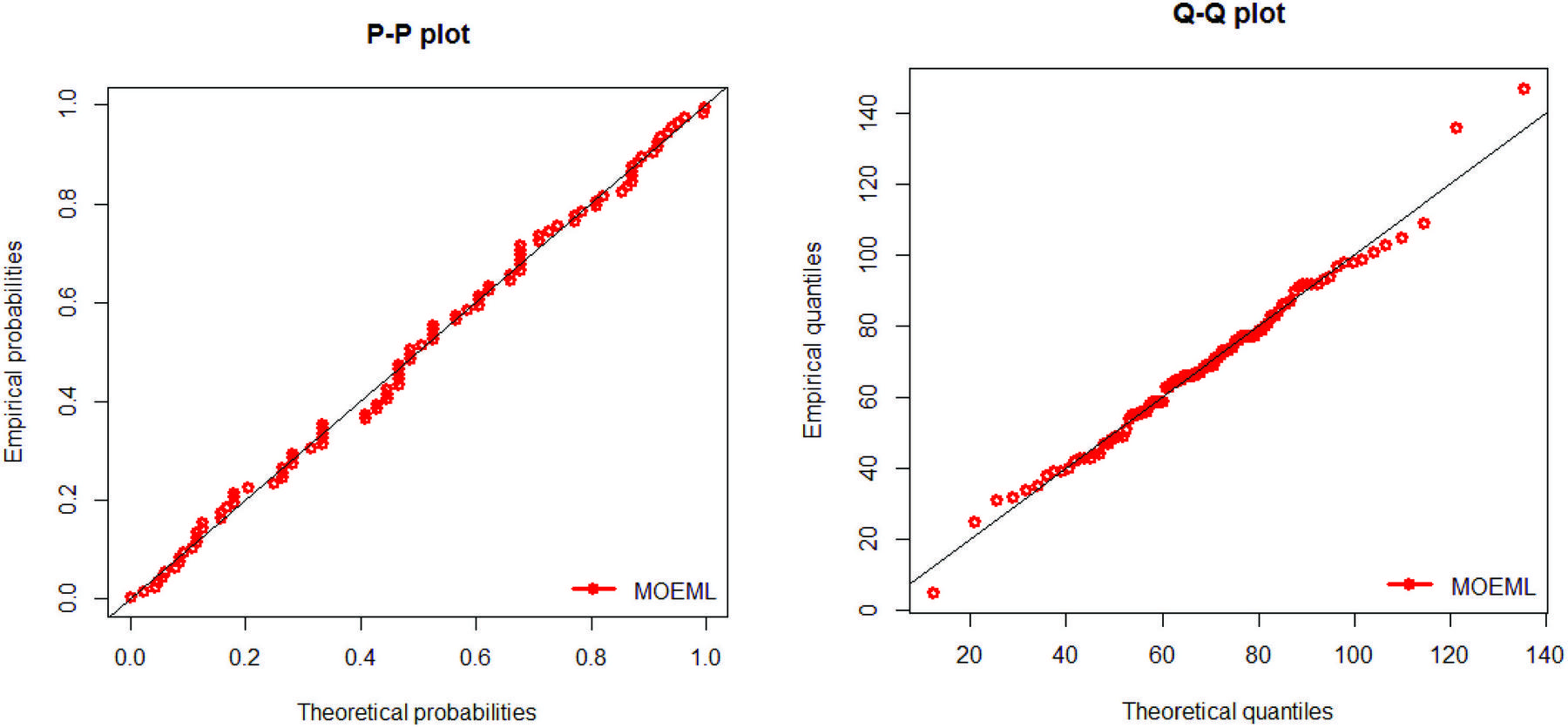
Figure 15 PP and QQ plots of MOEML for Dataset I.

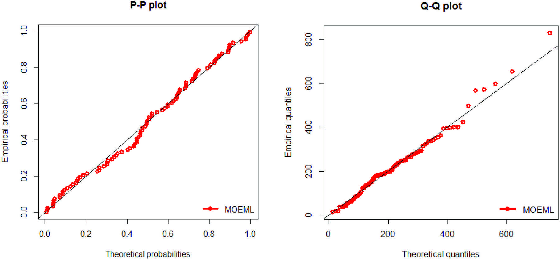
Figure 16 PP and QQ plots of MOEML for Dataset II.

Tables 2 and 3 summarize the findings of descriptive analysis for the specified distributions for Dataset I and II, respectively. The least $-\log \mathrm{L}$, AIC, BIC, AICc, K-S statistic and the highest $p$-values are acquired for the MOEML distribution. So, MOEML is the compatible model for two data sets. Figures 11 and 12 illustrate the estimated pdfs for Dataset  I and II, respectively. In addition, Figures 13 and 14 show the comparison of the cdfs for each model with the empirical distribution function. From plots, the proposed MOEML model furnishes the most agreeable fit for the specified data sets. Furthermore, the corresponding probability–probability (PP) and quantile-quantile (QQ) plots of MOEML for Dataset I and II are displayed in Figures 15 and 16, respectively. We remark that the scatter plot is well adjusted by the corresponding estimated line. Hence, from all graphical representations, the proposed model is more flexible than other considered distribution with respect to modeling lifetime data.

5.1 Conclusions

Lindley distribution has been practiced quite effectively in Statistics, because of its analytical tractability, providing an interesting alternative to the exponential distribution. In this present work, we discussed about a generalized version of a modified Lindley distribution. Several statistical and mathematical peculiarities of the MOEML model have been provided. The evaluation of the parameter is approached by the MLE method. The performance of estimates has been conferred via a simulation study. Further, we used two datasets to demonstrate the eminence of the MOEML model and compared it with other MOE models.

Acknowledgements

The authors would like to acknowledge the reviewers for their relevant opinions. The first author is thankful to the Department of Science and Technology (DST), Govt. of India for funding.

References

Al-Mutairi, D.K., Ghitany, M.E. and Kundu, D. (2013). Inferences on stress-strength reliability from Lindley distributions, Communications in Statistics - Theory and Methods, 42, pp. 1443–1463.

Birnbaum Z.W. and Saunders S.C. (1969). Estimation for a family of life distributions with applications to fatigue, Journal of Applied Probability, 6(2), pp. 328–347.

Castellares, F. and Lemonte, A.J. (2016). On the Marshall-Olkin extended distributions, Communications in Statistics-Theory and Methods. 45, pp. 4537–4555.

Chesneau, C., Tomy, L. and Gillariose, J. (2019a). A new modified Lindley distribution with properties and applications, preprint.

Chesneau, C., Tomy, L.and Jose, M. (2019b). Wrapped modified Lindley distribution, preprint.

Chesneau, C., Tomy, L., Gillariose, J. and Jamal, F. (2020). The inverted modified Lindley distribution, Journal of Statistical Theory and Practice, 14(46), pp. 1–17.

Cordeiro, G.M. Lemonte, A.J. and Ortega, E.M.M. (2014). The Marshall-Olkin family of distributions: mathematical properties and new models, Journal of Statistical Theory and Practice, 8, pp. 343–366.

Deniz, E.and Ojeda, E. (2011). The discrete lindley distribution: Properties and application. Journal of Statistical Computation and Simulation, 81(11), pp. 1405–1416.

Economou, P. and Caroni, C. (2007). Parametric proportional odds frailty models, Communications in Statistics-Simulation and Computation. 36, pp. 579–592.

Ghitany, M.E., Al-Awadhi, F.A. and Alkhalfan, L.A. (2007). Marshall-Olkin extended Lomax distribution and its application to censored data, Communications in Statistics-Theory and Methods, 36, pp. 1855–1866.

Ghitany, M.E., Atieh, B. and Nadarajah, S. (2008). Lindley distribution and its Applications, Mathematical Computation and Simulation, 78, 4, pp. 493–506.

Killer, A.Z. and Kamath A.R. (1982). Reliability analysis of CNC machine tools, Reliability Engineering, 3, pp. 449–473.

Krishna, E., Jose, K. K., Alice, T. and Ristic, M. M. (2013). Marshall-Olkin Frechet distribution, Communications in Statistics-Theory and Methods, 42, pp. 4091–4107.

Krishna, H. and Kumar, K. (2011). Reliability estimation in Lindley distribution with Progressive type II right censored sample, Journal Mathematics and Computers in Simulation archive, 82, (2), pp. 281–294.

Lam, K.F. and Leung, T.L. (2001). Marginal likelihood estimation for proportional odds models with right censored data, Lifetime Data Analysis, 7, pp. 39–54.

Leadbetter, M.R., Lindgren, G. and Rootzén H. (1987). Extremes and Related Properties of Random Sequences and Processes, New York, Springer Verlag.

Lindley, D.V. (1958). Fiducial distributions and Bayes theorem, Journal of the Royal Statistical Society, A(20), pp. 102–107.

Lindley, D.V. (1965). Introduction to Probability and Statistics from a Bayesian Viewpoint, Part II : inference, Cambridge University Press, New York.

Mahmoudi, E., Zakerzadeh, H. (2010). Generalized Poisson-Lindley distribution, Communications in Statistics-Theory and Methods, 39, pp. 1785–1798.

Marshall, A.W. and Olkin, I. (1997). A new method for adding a parameter to a family of distributions with application to the exponential and Weibull families, Biometrica, 84, pp. 641–652.

Merovci, F. (2013). Transmuted Lindley distribution, International Journal of Open Problems in Computer Science and Mathematics, 6, pp. 63–72.

Merovci, F. and Elbatal, I. (2014). Transmuted Lindley-geometric distribution and its applications, Journal of Statistics Applications & Probability, 3, pp. 77–91.

Merovci, F. and Sharma, V.K. (2014). The beta Lindley distribution: Properties and applications, Journal of Applied Mathematics 2014, pp. 1–10.

Nadarajah, S., Bakouch, H. and Tahmasbi, R. (2011). A generalized Lindley distribution, Sankhya B-Applied and Interdisciplinary Statistics, 73, pp. 331–359.

Nanda, A.K. and Das, S. (2012). Stochastic orders of the Marshall-Olkin extended distribution, Statistical Probability Letters, 82, pp. 295–302.

Oluyede, B.O. and Yang, T. (2015). A new class of generalized Lindley distributions with Applications, Journal of Statistical Computation and Simulation, 85, pp. 2072–2100.

Picciotto, R. (1970). Tensile fatigue characteristics of a sized polyester/viscose yarn and their effect on weaving performance, Master thesis, University of Raleigh, North Carolina State, USA.

Rao, G.S, and Mbwambo, S. (2019). Exponentiated inverse Rayleigh distribution and an application to coating weights of iron sheets data, Journal of Probability and Statistics, 2019(1), pp. 1–13.

Rubio, F.J. and Steel, M.F.J. (2012). On the Marshall-Olkin transformation as a skewing mechanism, Computational Statistical Data Analysis, 56, pp. 2251–2257.

Shanker, R., Hagos, F. and Sujatha, S. (2015). On modeling of lifetimes data using exponential and Lindley distributions, Biometrics & Biostatistics International Journal, 2(5), pp. 1–9.

Shanker, R. and Mishra, A. (2013). A two-parameter Lindley distribution, Statistics in Transition New Series, 14(1), pp. 45–56.

Sharma, V., Singh, S., Singh, U. and Agiwal, V. (2015). The inverse Lindley distribution: a stress-strength reliability model with applications to head and neck cancer data, Journal of Industrial and Production Engineering, 32(3), pp. 162–173.

Thomas, S.P., Jose K.K. and Tomy L. (2019). Discrete Harris Extended Lindley Distribution and Applications, preprint.

Tomy, L. (2018). A retrospective study on Lindley distribution, Biometrics and Biostatistics International Journal, 7(3), pp. 163–169.

Tomy, L., Jose K.K. and Thomas S.P. (2019). Harris Extended Lindley Distribution and Applications, preprint.

Biographies

Jiju Gillariose is a Research Scholar in the department of Statistics at St. Thomas College, Pala, Kerala, India affiliated to MG University, Kottayam. Her research deals with Distribution Theory, Data Analysis, Time Series and Statistical Quality Control.

Lishamol Tomy, Ph.D., is an Assistant Professor in the Department of Statistics, Deva Matha College Kuravilangad, Kerala State, South India. She is an approved Doctoral Research Supervisor of Mahatma Gandhi University Kottayam, in the Research Centre of Statistics, St. Thomas College Pala. She is a winner of the Jan Tinbergen Award for the Young Statisticians instituted by the International Statistical Institute, Netherlands. Her research interests are in Distribution Theory, Statistical Inferences, Time Series and Data Analysis.

Farrukh Jamal is currently Assistant Professor in the Department of Statistics, The Islamia University, Bahawalpur 63100, PAKISTAN. He worked as a lecturer in Government S.A. postgraduate College in 2012 to 2020, and Statistical Officer in Agriculture Department from 2007 to 2012. He received MSc and MPhil degrees in Statistics from the Islamia University of Bahawalpur (IU), Pakistan in 2003 and 2006. He has recently received PhD from IUB under the supervision of Dr. M. H. Tahir. He has 118 publications in his credit.

Christophe Chesneau, PhD in the field of applied mathematics specialising in statistics, at LPMA, University Paris 6, France. Christophe is working as specialist Statistics in the Department of Mathematics, LMNO, University of Caen Normandie. His research interests are in the areas of Statistical Inference, Nonparametric Statistics, Integer-Valued Time Series and Data Analysis.

Journal of Reliability and Statistical Studies, Vol. 13_1, 177–198.
doi: 10.13052/jrss0974-8024.1319
© 2020 River Publishers

Abstract

1 Background

2 MOE Modified Lindley Distribution

3 General Properties

3.1 Useful Expansions

3.2 Moments and Related Quantities

3.3 Mean Deviation (MD), Bonferroni and Lorenz Curves

4 Estimation Method with Simulation

4.1 Estimation Method

4.2 Simulation

5 Applications

5.1 Conclusions

Acknowledgements

References

Biographies