Parameters Estimation of the Exponentiated Chen Distribution Based on Upper Record Values

Farhad Yousaf^{1, 2}, Sajid Ali^1,*, Ismail Shah^{3, 1} and Saba Riaz⁴

¹Department of Statistics, Quaid-i-Azam University, Islamabad 45320, Pakistan
²Department of Social Sciences, University of Naples Federico II, Naples, Italy
³Department of Statistical Sciences, University of Padua, 35121, Padova, Italy
⁴Department of Statistics, Rawalpindi Women University, 6th Road, Satellite Town, Rawalpindi, Punjab, Pakistan
E-mail: farhadyousaf@stat.qau.edu.pk; farhad.yousaf@unina.it; sajidali.qau@hotmail.com; shah@unipd.it; ishah@qau.edu.pk; saba.riaz@f.rwu.edu.pk
*Corresponding Author

Abstract

This article discusses the Bayesian and frequentist inferences for the exponentiated Chen distribution assuming upper record values. Due to unavailability of the compact form of marginal posterior distributions, a Markov Chain Monte Carlo algorithm is designed to compute the posterior summaries. Prediction of future record values under Bayesian and frequentist methods is also discussed mathematically and numerically. Further, a sensitivity analysis to assess the effect of prior on the estimated parameters is also a part of this study. Besides the simulation studies, the importance of the present study is illustrated with the help of a real data example. It is noted that the Bayes estimates outperform the frequentist inference.

Keywords: Asymptotic intervals, Bayesian prediction, exponentiated Chen distribution, record values.

1 Introduction

The ordered observations which strictly exceed the previous values are called the record values, and thus the record statistics are closely related to theory of order statistics. The study of records gained popularity in the literature because of their practical usage, such as industrial stress testing, meteorology, seismology, hydrology, sporting events, economics, life testing, oil and mining surveys (Ahsanullah and Nevzorov, 2015). In statistics, Chandler (1952) developed the concept of record statistics and also discuss record values, record times and inter record times. After that numerous studies discussed record values and related statistical inference. For instance, Dziubdziela and Kopociński (1976), Nagaraja (1977), Srivastava (1979), Nevzorov (1988), Arshad and Jamal (2019), Yousaf et al. (2019), etc. For more detailed information on record statistics, and their applications, we refer to Arnold et al. (2011) and Ahsanullah and Nevzorov (2015). Soliman and Al-Aboud (2008) used upper record values from a Rayleigh distribution and discussed Bayesian and non-Bayesian approaches to obtain the estimators of the parameter. Seo and Kim (2017) discussed objective Bayesian analysis based on upper record values from two-parameter Rayleigh distribution with partial information. The authors provided a pivotal quantity and an algorithm based on the pivotal quantity to predict the behavior of future survival records. Al-Duais (2021) used the inverse Weibull distribution for the Bayesian analysis of upper record values using balanced loss function. Pak et al. (2022) considered the records as well as the corresponding inter-record times to develop inference procedures for $R=P(X>Y)$ assuming $X$ and $Y$ come from Weibull distribution. Kumar and Gupta (2023) discussed Bayesian analysis of inverse Rayleigh distribution using noninformative prior for different loss functions. Alhamidah et al. (2023) considered the problem of E-Bayesian estimation and its expected posterior mean squared error (E-PMSE) in a Burr type XII model on the basis of record values.

The exponentiated Chen distribution (ECD) is introduced by Chaubey and Zhang (2015), which is in fact is an extension of the two-parameter Chen distribution (Chen, 2000). The ECD is a positively skewed and more flexible than the two-parameter Chen model. The ECD has a bathtub hazard function, which decrease initially, then remains constant, and finally increase. In practice, the most accurate failure rate is bathtub-shaped, and in the literature, many researchers proposed different models for bathtub-shaped hazard rate, see, for example, Hjorth (1980), Rajarshi and Rajarshi (1988), Xie and Lai (1996), Chen (2000), and references cited therein.

Suppose $X_1,X_2,\mathrm{\dots },X_n$ be the $n$ upper record values from the ECD with probability density function

$g(x;\gamma ,\mu ,\phi )$	$=\gamma \mu \phi x^{\mu -1}\exp (x^{\mu })\exp (\phi (1-\exp (x^{\mu })))$
	$\mathrm{\hspace{1em}}(1-\exp (\phi (1-\exp (x^{\mu }))){)}^{\gamma -1}$
	$x\ge 0,\gamma ,\mu ,\phi >0$	(1)

where $\phi >0$ is the scale and $\gamma ,\mu >0$ are the shape parameters. By setting $\gamma$ = 1 in Equation (1), the distribution reduces to

$g(x)=\mu \phi x^{\mu -1}\exp (x^{\mu })\exp (\phi (1-\exp (x^{\mu })))\mathit{\hspace{1em}\hspace{1em}}x,\mu ,\phi >0$

(2)

which is the two-parameter Chen distribution. Thus, the Chen distribution is a special case of the ECD. The distribution function of the ECD is given as

$G(x;\gamma ,\mu ,\phi )={(1-\exp (\phi (1-\exp (x^{\mu }))))}^{\gamma }\mathit{\hspace{1em}\hspace{1em}}x\ge 0$

(3)

The hazard, reliability, and quantile function of ECD are given, respectively, by

$h(x)$	$={\displaystyle \frac{\begin{array}{c}\gamma \mu \phi x^{\mu -1}\exp (x^{\mu })\exp (\phi (1-\exp (x^{\mu })))\hfill \\ {(1-\exp (\phi (1-\exp (x^{\mu }))))}^{\gamma -1}\hfill \end{array}}{1-{(1-\exp (\phi (1-\exp (x^{\mu }))))}^{\gamma }}}\mathit{\hspace{1em}}x\ge 0,\mu ,\phi >0$
$R(x)$	$=1-{(1-\exp (\phi (1-\exp (x^{\mu }))))}^{\gamma }\mathit{\hspace{1em}\hspace{1em}}x\ge 0,\mu ,\phi >0$	(4)
$X_w$	$={\left[\log \left(1-{\displaystyle \frac{1}{\phi }}\log (1-w^{1/\gamma })\right)\right]}^{1/\mu }\mathit{\hspace{1em}\hspace{1em}}w\in (0,1)$	(5)

The graphical depiction of the ECD and its failure is given in Figure 1. To be more specific, the plot on the left, i.e., Figure 1(a), is the probability density function plot of the ECD with parameters $\gamma =35,\mu =0.25,\phi =1$ plotted as the yellow solid line, $\gamma =35,\mu =0.25,\phi =1.5$ plotted as the red dashed line, $\gamma =35,\mu =0.25,\phi =2$ plotted as the green dotted line, $\gamma =35,\mu =0.25,\phi =2.5$ plotted as the blue dot-dashed line and finally, $\gamma =35,\mu =0.25,\phi =3$ plotted as the gray long-dashed line. Similarly, in Figure 1(b) the hazard function is plotted assuming the scale and the first shape parameter fixed at $\gamma =35,\mu =0.25$, while assuming the second shape parameter $\phi$ = 1, 1.5, 2, 2.5 and 3, respectively.

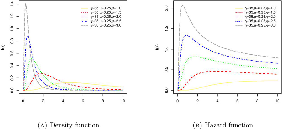
Figure 1 Density and hazard plots for different parameter values.

The development of new probability models and studying their different properties has gained a lot of attention from research during the last decade. For example, Xie et al. (2002) introduced the three-parameter Weibull distribution by adding a new scale parameter to baseline distribution. Later, Chaubey and Zhang (2015) also extended the Chen distribution by adding the shape parameter and named the proposed distribution as the ECD. Dey et al. (2017) studied different properties and estimation methods for the ECD and concluded that the maximum product of spacing (MPS) method is more efficient than the other estimation methods. Khan et al. (2016) introduced the transmuted exponentiated distribution. Recently, Khan et al. (2018) introduced a new five parameter Kumaraswamy exponentiated Chen distribution by adding two new shape parameters to the base line ECD. Eliwa et al. (2021) proposed exponentiated odd Chen-G family of distribution and studied different properties. Later, Awodutire (2022) used the exponential distribution as a baseline distribution to study the properties of exponentiated odd Chen-G family. Recently, Azimi et al. (2023) proposed inverted exponentiated Chen distribution with application to cancer data. Méndez-González et al. (2023) introduced the additive Chen distribution and discussed its properties and applications.

The aim of this study is to present parameter estimation of the ECD based on upper record values under Bayesian and non-Bayesian methods. Further, a framework for prediction of the future record observations is also discussed. As we have shown in the next section, Bayesian computations cannot be done in the traditional manner, a Markov Chain Monte Carlo (MCMC) algorithm is devised to obtain different posterior summaries.

The rest of the study is organized as follows. Section 2 derives the estimators of the unknown parameters for the ECD by the maximum likelihood method. Section 3 discusses Bayes estimators under the squared error loss function (SELF) using informative and non-informative priors. Sensitivity analysis is discussed in Section 4. The prediction of future record values for the ECD under Bayesian and frequentist approaches is discussed in Section 5. The numerical results of simulated as well as for real data are presented in Sections 6 and 7, respectively. Finally, Section 8 presents conclusion.

2 Maximum Likelihood Estimation

For the estimation of $\gamma ,\mu$ and $\phi$ assuming the upper record values using the maximum likelihood estimation method, suppose $X_1,X_2,X_3,\mathrm{\dots }$ be a sequence of independent and identically distributed (iid) random variables with PDF $g(x)$ and CDF $G(x)$ from the Exponentiated Chen distribution. Suppose $Y_n=\max (\min )\{X_1,X_2,X_3,\mathrm{\dots },X_n\}$ for $n\ge 0$. The observation $X_k$ is an upper(lower) record value of this sequence if $Y_k>(<)Y_{k-1},k>1$, i.e., $X_k$ is the upper(lower) value if its value is greater(smaller) than that of all the preceding observations, where $X_{k_{(n)}}$ and $k_{(n)}$ denote the upper record values and upper record times, respectively. Assuming a sample of size $n$ record values $X=\{X_{k_{(1)}},X_{k_{(2)}},\mathrm{\cdots },X_{k_{(n)}}\}$ from Equation (1), the likelihood can be written as (Ahsanullah, 1995).

$$L(\gamma ,\mu ,\phi |x)=g(x_{k(n)};\gamma ,\mu ,\phi )\prod _{i=1}^{n-1}\frac{g(x_{k(i)};\gamma ,\mu ,\phi )}{1-G(x_{k(i)},\gamma ,\mu ,\phi )}$$
$$0\le x_{k(1)}<x_{k(2)}<\mathrm{\cdots }<x_{k(n)}<\mathrm{\infty }$$	(6)

By replacing the PDF and CDF of the ECD in Equation (6), the likelihood function can be written as

$L(\gamma ,\mu ,\phi |\mathbf{\text{x}})={\gamma }^n{\mu }^n{\phi }^n{\displaystyle \frac{\begin{array}{c}{\prod }_{i=1}^n{x}_{k(i)}^{\mu -1}\exp (x_{k(i)}^{\mu })\exp \left[\phi \left\{1-\exp (x_{k(i)}^{\mu })\right\}\right]\hfill \\ {\left[1-\exp \left\{\phi \left(1-\exp (x_{k(i)}^{\mu })\right)\right\}\right]}^{\gamma -1}\hfill \end{array}}{{\prod }_{i=1}^{n-1}[1-{\{1-\exp (\phi (1-\exp (x_{k(i)}^{\mu })))\}}^{\gamma }]}}$

(7)

2.1 Likelihood Estimators

For deriving the maximum likelihood estimators (MLE), take the partial derivatives of the logarithm of the likelihood function $l(\gamma ,\mu ,\phi |x)=\log L(\gamma ,\mu ,\phi |\mathbf{\text{x}})$ with respect to unknown parameters. It is to be noted that the terms without $\gamma ,\mu$ and $\phi$ can be ignored.

$l(\gamma ,\mu ,\phi |x)$	$=n\log (\gamma )+n\log (\mu )+n\log (\phi )+{\displaystyle \sum _{i=1}^n}{x}_{k(i)}^{\mu }$
	$\mathrm{\hspace{1em}}+(\gamma -1){\displaystyle \sum _{i=1}^n}\log (1-\exp (\phi (1-\exp (x_{k(i)}^{\mu }))))$
	$\mathrm{\hspace{1em}}+(\mu -1){\displaystyle \sum _{i=1}^n}\log (x_{k(i)})$
	$\mathrm{\hspace{1em}}-{\displaystyle \sum _{i=1}^{n-1}}\log \left(1-{(1-\exp (\phi (1-\exp (x_{k(i)}^{\mu }))))}^{\gamma }\right)$
	$\mathrm{\hspace{1em}}+\phi {\displaystyle \sum _{i=1}^n}(1-\exp (x_{k(i)}^{\mu }))$	(8)

Next, partially differentiate Equation (7) with respect to the parameters and equating the resulting equations to zero. The resulting normal equations can be written as.

${\displaystyle \frac{n}{\gamma }}-{\displaystyle \sum _{i=1}^{n-1}}{\displaystyle \frac{\log (1-\exp {(\phi (1-\exp (x_{k(i)}^{\mu })))}^{\gamma }\log (1-\exp (\phi (1-\exp (x_{k(i)}^{\mu })))}{1-{(1-\exp (\phi (1-\exp (x_{k(i)}^{\mu }))))}^{\gamma }}}$
$\mathrm{\hspace{1em}\hspace{1em}}+{\displaystyle \sum _{i=1}^n}\log (1-\exp (\phi (1-\exp (x_{k(i)}^{\mu })))=0$	(9)
${\displaystyle \frac{n}{\mu }}+{\displaystyle \sum _{i=1}^n}\log (x_{k(i)})+{\displaystyle \sum _{i=1}^n}{x}_{k(i)}^{\mu }\log (x_{k(i)})+(\gamma -1)$
$\mathrm{\hspace{1em}\hspace{1em}}{\displaystyle \sum _{i=1}^n}{\displaystyle \frac{\phi x_{k(i)}^{\mu }\log (x_{k(i)})\exp (\phi (1-\exp (x_{k(i)}^{\mu }))+x_{k(i)}^{\mu })}{1-\exp (\phi (1-\exp (x_{k(i)}^{\mu })))}}$
$\mathrm{\hspace{1em}\hspace{1em}}-{\displaystyle \sum _{i=1}^{n-1}}{\displaystyle \frac{\begin{array}{c}\gamma \phi x_{k(i)}^{\mu }\log (x_{k(i)})\exp (\phi (1-\exp (x_{k(i)}^{\mu }))+x_{k(i)}^{\mu })\hfill \\ {(1-\exp (\phi (1-\exp (x_{k(i)}^{\mu }))))}^{\gamma -1}\hfill \end{array}}{1-{(1-\exp (\phi (1-\exp (x_{k(i)}^{\mu }))))}^{\gamma }}}$
$\mathrm{\hspace{1em}\hspace{1em}}+{\displaystyle \sum _{i=1}^n}\log (x_{k(i)})-\phi {\displaystyle \sum _{i=1}^n}\exp (x_{k(i)}^{\mu })x_{k(i)}^{\mu }\log (x_{k(i)})=0$	(10)
${\displaystyle \frac{n}{\phi }}-{\displaystyle \sum _{i=1}^{n-1}}{\displaystyle \frac{\begin{array}{c}\gamma (1-\exp (x_{k(i)}^{\mu }))\exp (\phi (1-\exp (x_{k(i)}^{\mu })))\hfill \\ {(1-\exp (\phi (1-\exp (x_{k(i)}^{\mu }))))}^{\gamma -1}\hfill \end{array}}{1-{(1-\exp (\phi (1-\exp (x_{k(i)}^{\mu }))))}^{\gamma }}}$
$\mathrm{\hspace{1em}\hspace{1em}}+{\displaystyle \sum _{i=1}^n}(1-\exp (x_{k(i)}^{\mu }))-(\gamma -1)$
$\mathrm{\hspace{1em}\hspace{1em}}{\displaystyle \sum _{i=1}^n}{\displaystyle \frac{(1-\exp (x_{k(i)}^{\mu }))\exp (\phi (1-\exp (x_{k(i)}^{\mu })))}{1-\exp (\phi (1-\exp (x_{k(i)}^{\mu })))}}=0$	(11)

Solving Equations (9)–(11), one can get the MLE for the ECD parameters $\gamma ,\mu$ and $\phi$, denoted as ${\widehat{\gamma }}_{\mathit{MLE}}$, ${\widehat{\mu }}_{\mathit{MLE}}$ and ${\widehat{\phi }}_{MLE}$, respectively. An iterative procedure like Newton Raphson is suggested to solve the above equations because these equations do not have analytical solution.

2.2 Asymptotic Confidence Intervals

Since the MLE of $\gamma ,\mu$ and $\phi$ cannot be solved analytically, the exact distribution of these estimators is difficult to obtain. Therefore, the exact confidence intervals for the parameters $\gamma ,\mu$ and $\phi$ cannot be obtained. Alternatively, asymptotic confidence intervals are obtained by using the large sample approximation. It is well known fact that the asymptotic distribution of the MLE, say, $\psi$ is $(\widehat{\psi }-\psi )\to N(\psi ,I^{-1}(\psi ))$ (Lawless, 2011), where $I^{-1}(\psi )$ is the inverse of the observed Fisher information matrix of the unknown parameters $\psi$ = $(\gamma ,\mu ,\phi )$, defined as

$I^{-1}={\left(\begin{array}{ccccc}\hfill -\frac{{\partial }^{2}l(\gamma ,\mu ,\phi |\mathbf{x})}{\partial {\gamma }^2}\hfill & \hfill \hfill & \hfill -\frac{{\partial }^{2}l(\gamma ,\mu ,\phi |\mathbf{x})}{\partial \gamma \partial \mu }\hfill & \hfill \hfill & \hfill -\frac{{\partial }^{2}l(\gamma ,\mu ,\phi |\mathbf{x})}{\partial \gamma \partial \phi }\hfill \\ \hfill -\frac{{\partial }^{2}l(\gamma ,\mu ,\phi |\mathbf{x})}{\partial \mu \partial \gamma }\hfill & \hfill \hfill & \hfill -\frac{{\partial }^{2}l(\gamma ,\mu ,\phi |\mathbf{x})}{\partial {\mu }^2}\hfill & \hfill \hfill & \hfill -\frac{{\partial }^{2}l(\gamma ,\mu ,\phi |\mathbf{x})}{\partial \mu \partial \phi }\hfill \\ \hfill -\frac{{\partial }^{2}l(\gamma ,\mu ,\phi |\mathbf{x})}{\partial \phi \partial \gamma }\hfill & \hfill \hfill & \hfill -\frac{{\partial }^{2}l(\gamma ,\mu ,\phi |\mathbf{x})}{\partial \phi \partial \mu }\hfill & \hfill \hfill & \hfill -\frac{{\partial }^{2}l(\gamma ,\mu ,\phi |\mathbf{x})}{\partial {\phi }^2}\hfill \end{array}\right)|}_{(\gamma ,\mu ,\phi )=(\widehat{\gamma },\widehat{\mu },\widehat{\phi })}^{-1}$

or

$I^{-1}=\left(\begin{array}{ccccc}\hfill var(\widehat{\gamma })\hfill & \hfill \hfill & \hfill cov(\widehat{\gamma },\widehat{\mu })\hfill & \hfill \hfill & \hfill cov(\widehat{\gamma },\widehat{\phi })\hfill \\ \hfill cov(\widehat{\mu },\widehat{\gamma })\hfill & \hfill \hfill & \hfill var(\widehat{\mu })\hfill & \hfill \hfill & \hfill cov(\widehat{\mu },\widehat{\phi })\hfill \\ \hfill cov(\widehat{\phi },\widehat{\gamma })\hfill & \hfill \hfill & \hfill cov(\widehat{\phi },\widehat{\mu })\hfill & \hfill \hfill & \hfill var(\widehat{\phi })\hfill \end{array}\right)$

where

${\displaystyle \frac{{\partial }^{2}l(\gamma ,\mu ,\phi |\mathbf{x})}{\partial {\gamma }^2}}$	$={\displaystyle \frac{\partial }{\partial \gamma }}\left({\displaystyle \frac{\partial l(\gamma ,\mu ,\phi |x)}{\partial \gamma }}\right),$
${\displaystyle \frac{{\partial }^{2}l(\gamma ,\mu ,\phi |\mathbf{x})}{\partial \gamma \partial \mu }}$	$={\displaystyle \frac{\partial }{\partial \gamma }}\left({\displaystyle \frac{\partial l(\gamma ,\mu ,\phi |x)}{\partial \mu }}\right)$
${\displaystyle \frac{{\partial }^{2}l(\gamma ,\mu ,\phi |\mathbf{x})}{\partial {\mu }^2}}$	$={\displaystyle \frac{\partial }{\partial \mu }}\left({\displaystyle \frac{\partial l(\gamma ,\mu ,\phi |x)}{\partial \mu }}\right),$
${\displaystyle \frac{{\partial }^{2}l(\gamma ,\mu ,\phi |\mathbf{x})}{\partial \mu \partial \phi }}$	$={\displaystyle \frac{\partial }{\partial \mu }}\left({\displaystyle \frac{\partial l(\gamma ,\mu ,\phi |x)}{\partial \phi }}\right)$
${\displaystyle \frac{{\partial }^{2}l(\gamma ,\mu ,\phi |\mathbf{x})}{\partial {\phi }^2}}$	$={\displaystyle \frac{\partial }{\partial \phi }}\left({\displaystyle \frac{\partial l(\gamma ,\mu ,\phi |x)}{\partial \phi }}\right),$
${\displaystyle \frac{{\partial }^{2}l(\phi ,\mu ,\gamma |\mathbf{x})}{\partial \phi \partial \gamma }}$	$={\displaystyle \frac{\partial }{\partial \phi }}\left({\displaystyle \frac{\partial l(\gamma ,\mu ,\phi |x)}{\partial \gamma }}\right)$

The asymptotic $100(1-\psi )\%$ confidence intervals of the parameter $\gamma ,\mu$ and $\phi$ are of the forms

$\widehat{\gamma }\pm z_{\psi /2}\sqrt{var(\widehat{\gamma })}$

$\widehat{\mu }\pm z_{\psi /2}\sqrt{var(\widehat{\mu })}$

and

$$\widehat{\phi }\pm z_{\psi /2}\sqrt{var(\widehat{\phi })}$$

where $z_{\psi /2}$ is the upper $(\psi /2)th$ percentile of the standard normal distribution.

3 Bayesian Estimation

The aim of this section is to present Bayesian analysis for the unknown parameters of the ECD based on the upper record values. Selection of a suitable prior for the unknown parameters is an important task in Bayesian inference. There are many types of priors, like informative and non-informative priors which can be used in the Bayesian inference. A sufficient knowledge about a problem at hand is known to be the informative prior while vice versa for the noninformative prior case. The Bayes theorem is used to combine the currently observed information with the prior information to get an updated form of the information, which is known as the posterior distribution. For simplicity, in this study it is assumed that the parameters $\gamma ,\mu$ and $\phi$ are independent and follow gamma distribution, i.e., $\gamma \sim$ gamma(a,b), $\mu \sim$ gamma(c,d) and $\phi \sim$ gamma(e,f) with PDFs

$g(\gamma )\propto {\gamma }^{a-1}\exp (-b\gamma )\mathit{\hspace{1em}\hspace{1em}\hspace{1em}\hspace{1em}}\gamma >0$	(12)
$g(\mu )\propto {\mu }^{c-1}\exp (-d\mu )\mathit{\hspace{1em}\hspace{1em}\hspace{1em}\hspace{1em}}\mu >0$	(13)

and

$$g(\phi )\propto {\phi }^{e-1}\exp (-f\phi )\mathit{\hspace{1em}\hspace{1em}\hspace{1em}\hspace{1em}}\phi >0$$

(14)

where a, b, c, d, e and f are known and non-negative hyperparameters. It is worth mentioning that the gamma prior is considered for illustration and any other suitable prior can be used instead of this. Furthermore, dependent type priors can also be assumed. To this end, the joint prior distribution can be written as follows.

$$g(\gamma ,\mu ,\phi )\propto {\gamma }^{a-1}\exp (-b\gamma ){\mu }^{c-1}\exp (-d\mu ){\phi }^{e-1}\exp (-f\phi )$$
$$\gamma ,\mu ,\phi >0$$	(15)

The joint posterior distribution is obtained by combining Equation (7) and Equation (15) and the resulting expression is given in Equation (16).

$$\pi (\gamma ,\mu ,\phi |\mathbf{x})\propto L(\gamma ,\mu ,\phi |x)\times g(\gamma ,\mu ,\phi )$$
$$\pi (\gamma ,\mu ,\phi |\mathbf{x})\propto {\gamma }^{n+a-1}{\mu }^{n+c-1}{\phi }^{n+e-1}\exp (-b\gamma -d\mu -f\phi )T$$	(16)

where

$T={\displaystyle \frac{\begin{array}{c}{\sum }_{i=1}^n{x}_{k(i)}^{\mu -1}\exp (x_{k(i)}^{\mu })\exp (\phi (1-\exp (x_{k(i)}^{\mu })))\hfill \\ (1-\exp {(\phi (1-\exp (x_{k(i)}^{\mu })))}^{\gamma -1}\hfill \end{array}}{{\sum }_{i=1}^{n-1}(1-{(1-\exp (\phi (1-\exp (x_{k(i)}^{\mu }))))}^{\gamma })}}$

(17)

For deriving the marginal posterior distribution of the parameter of interest, integrate the joint posterior distribution with respect to nuisance parameters. The marginal posterior distribution of $\gamma ,\mu$ and $\phi$ can be written as follows.

${\pi }_1(\gamma |\mathbf{x})$	$\propto {\gamma }^{n+a-1}\exp (-b\gamma ){\displaystyle {\int }_0^{\mathrm{\infty }}}{\displaystyle {\int }_0^{\mathrm{\infty }}}{\mu }^{n+c-1}{\phi }^{n+e-1}$
	$\mathrm{\hspace{1em}}\times \exp (-d\mu -f\phi )Td\mu d\phi$	(18)
${\pi }_2(\mu |\mathbf{x})$	$\propto {\mu }^{n+c-1}\exp (-d\mu ){\displaystyle {\int }_0^{\mathrm{\infty }}}{\displaystyle {\int }_0^{\mathrm{\infty }}}{\mu }^{n+c-1}{\phi }^{n+a-1}$
	$\mathrm{\hspace{1em}}\times \exp (-b\gamma -f\phi )Td\gamma d\phi$	(19)

and

${\pi }_3(\phi |\mathbf{x})$	$\propto {\phi }^{n+e-1}\exp (-f\phi ){\displaystyle {\int }_0^{\mathrm{\infty }}}{\displaystyle {\int }_0^{\mathrm{\infty }}}{\gamma }^{n+a-1}{\mu }^{n+c-1}$
	$\mathrm{\hspace{1em}}\times \exp (-b\gamma -d\mu )Td\gamma d\mu$	(20)

Next, the specification of a suitable loss function is required to estimate the unknown parameters. In Bayesian, one of the most commonly used loss function is the squared error loss function (SELF). Assuming the SELF, the Bayes estimators for the parameter $\gamma$, $\mu$ and $\phi$ can be obtained as ${\widehat{\gamma }}_{\mathit{BGE}}=E_{\gamma |\mathbf{x}}(\gamma )$, ${\widehat{\mu }}_{\mathit{BGE}}=E_{\mu |\mathbf{x}}(\mu )$ and ${\widehat{\phi }}_{\mathit{BGE}}=E_{\phi |\mathbf{x}}(\phi )$, respectively, provided that $E(\gamma )$, $E(\mu )$ and $E(\phi )$ are finite and do exist. These estimators can be written as ${\widehat{\gamma }}_{\mathit{BGE}}=T_{\gamma }$, ${\widehat{\mu }}_{\mathit{BGE}}=T_{\mu }$ and ${\widehat{\gamma }}_{\mathit{BGE}}=T_{\phi }$ where

$T_{\gamma }$	$={\displaystyle {\int }_0^{\mathrm{\infty }}}{\displaystyle {\int }_0^{\mathrm{\infty }}}{\displaystyle {\int }_0^{\mathrm{\infty }}}{\gamma }^{n+a}{\mu }^{n+c-1}{\phi }^{n+e-1}\exp (-b\gamma -d\mu -f\phi )T\mathit{d}\gamma \mathit{d}\mu \mathit{d}\phi$	(21)
$T_{\mu }$	$={\displaystyle {\int }_0^{\mathrm{\infty }}}{\displaystyle {\int }_0^{\mathrm{\infty }}}{\displaystyle {\int }_0^{\mathrm{\infty }}}{\gamma }^{n+a-1}{\mu }^{n+c}{\phi }^{n+e-1}\exp (-b\gamma -d\mu -f\phi )T\mathit{d}\gamma \mathit{d}\mu \mathit{d}\phi$	(22)

and

$T_{\phi }={\displaystyle {\int }_0^{\mathrm{\infty }}}{\displaystyle {\int }_0^{\mathrm{\infty }}}{\displaystyle {\int }_0^{\mathrm{\infty }}}{\gamma }^{n+a-1}{\mu }^{n+c-1}{\phi }^{n+e}\exp (-b\gamma -d\mu -f\phi )T\mathit{d}\gamma \mathit{d}\mu \mathit{d}\phi$

(23)

Since the Bayes estimators cannot be obtained analytically, a numerical procedure is required to solve them numerically. To this end, the use of Metropolis-Hastings (MH) algorithm is suggested to obtain the Bayes estimators. Within Markov Chain Monte Carlo (MCMC), Metropolis algorithm is a very flexible method to obtain Bayes estimates (Metropolis et al., 1953; Hastings, 1970). We use MH algorithm to generate the parameter $\gamma$ because its distribution is not a well-known distribution. We express the marginal posterior distribution of each parameter as follows

$g(\gamma |\mu ,\phi ,\mathbf{x})$	$\sim {\gamma }^{n+a-1}\exp (-b\gamma ){\displaystyle \sum _{i=1}^n}$
	$\mathrm{\hspace{1em}}\times \exp (x_{k(i)}^{\mu }){\displaystyle \frac{{\sum }_{i=1}^n{(1-\exp (\phi (1-\exp (x_{k(i)}^{\mu }))))}^{\gamma -1}}{{\sum }_{i=1}^{n-1}(1-{(1-\exp (\phi (1-\exp (x_{k(i)}^{\mu }))))}^{\gamma })}}$	(24)
$g(\mu |\mathbf{x})$	$\sim \text{Gamma}(n+c,d+\ln {\displaystyle \frac{1}{{\sum }_{i=1}^n{x}_{k(i)}}})$	(25)

and

$$g(\phi |\mathbf{x})\sim \text{Gamma}(n+e,f-(1-\exp (x_{k(i)}^{\mu }))$$

(26)

To apply the MH algorithm, first, initialize the parameter $\gamma$ as the initial value ${\gamma }_{\tau }$ and draw the next value ${\gamma }^{\prime }$ with probability density $g({\gamma }^{\prime }|{\gamma }_{\tau })$ which is known as the transition kernel. It is to be noted that gamma distribution is taken as a transition kernel for illustration and any other suitable distribution can be considered. Then, calculate $m=\min (m_1{m}_2,1)$, where $m_1=g({\gamma }^{\prime })/g({\gamma }_{\tau })$ defining the probability ratio between the present and the last sample ${\gamma }_{\tau }$, and $m_2=\frac{g({\gamma }_{\tau }|{\gamma }^{\prime })}{g({\gamma }^{\prime }|{\gamma }_{\tau })}$. If the result of $m_2=1$, the density is symmetric. A new state is rejected if $m=1$, ${\gamma }_{\tau +1}={\gamma }^{\prime }$, i.e.,

${\gamma }_{\tau +1}=\{\begin{array}{c}\hfill {\gamma }^{\prime }\hspace{1em}\hspace{1em}\text{with probability m}\hfill \\ \hfill {\gamma }_{\tau }\hspace{1em}\hspace{1em}\text{with probability 1-m}\hfill \end{array}$

To diminish the effect of initial state, repeat the above process a large number of times. To obtain more reliable results, some initial state values can be discarded which is known as the burn-in period. The Markov Chain will converge when the variance of the parameter values decreased or becomes too small. We suggest the following steps to calculate the posterior estimates.

(1) Guess the initial value of $\gamma$ as ${\gamma }_0$.

(2) Generate $\mu$ and $\phi$ from $g(\mu |\mathbf{x})$ and $g(\phi |\mathbf{x})$.

(a) To calculate $\gamma$, estimate the acceptance probability by $g({\gamma }^{(i)},{\gamma }^{\prime })=\min (1,\frac{g({\gamma }^{\prime }|\mathbf{x})g({\gamma }^{(i)}|{\gamma }^{\prime })}{g({\gamma }^{(i)}|\mathbf{x})g({\gamma }^{\prime }|{\gamma }^{(i)})})$, where $g(\gamma |\mathbf{x})$ has been defined above.

(b) Generate random numbers U(0,1).

(c) If $g({\gamma }^{(i)},{\gamma }^{\prime })\ge U,{\gamma }^{(i+1)}={\gamma }^{(i)}$

(3) Suppose $\gamma$, $\mu$ and $\phi$ take the values ${\gamma }_i,{\mu }_i$ and ${\phi }_i$ at the ith step. Now, one can generate $g({\gamma }_{i+1}|{\gamma }_i,{\mu }_i,{\phi }_i,\mathbf{x})$.

(4) Repeat the above steps N-times.

(5) Obtain the Bayes estimators of $h(\gamma ,\mu ,\phi )$ by $\frac{1}{K-L}{\sum }_{i=L+1}^{K}g({\gamma }_{\tau },{\mu }_{\tau }$, ${\phi }_{\tau })$, where L denote the number of burn-in sample.

A great advantage of the MH approach over Gibbs sampler is that the conditional distribution of parameters is notessential. In this study, we considered 50,000 as the MCMC iteration size and first 5,000 observations were discarded as the burn-in samples.

3.1 Bayes Intervals

This section discusses the Bayes intervals, which give a probabilistic statement with a specified probability whether a parameter of interest is included in the intervals or not. Thus, Bayes intervals do not depend on the repetition concept as the classical intervals and also known as the credible intervals. After deriving the marginal posterior distribution of the parameter $\gamma$, a symmetric $100(1-\varphi )\%$ two-sided Bayes interval estimate of $\gamma$, denoted by $[{\gamma }_L,{\gamma }_U]$, can be obtained by solving the following two equations (Martz and Waller, 1982).

$${\int }_0^{{\gamma }_L}{\pi }_1(\omega |\mathbf{x})\mathit{d}\omega =\frac{\varphi }{2}$$

(27)

and

$${\int }_{{\gamma }_U}^{\mathrm{\infty }}{\pi }_1(\omega |\mathbf{x})\mathit{d}\omega =\frac{\varphi }{2}$$

(28)

for the limits ${\gamma }_L$ and ${\gamma }_U$, and subject to ${\pi }_1({\gamma }_L|\mathbf{x})={\pi }_1({\gamma }_U|\mathbf{x})$. Similarly, a $100(1-\varphi /2)\%$ two-sided Bayes interval estimate of $\mu$, denoted by $[{\mu }_L,{\mu }_U]$, can be obtained by solving

$${\int }_0^{{\mu }_L}{\pi }_2(\omega |\mathbf{x})\mathit{d}\omega =\frac{\varphi }{2}$$

(29)

and

$${\int }_{{\mu }_U}^{\mathrm{\infty }}{\pi }_2(\omega |\mathbf{x})\mathit{d}\omega =\frac{\varphi }{2}$$

(30)

for the limits ${\mu }_L$ and ${\mu }_U$ subject to ${\pi }_2({\mu }_L|\mathbf{x})={\pi }_2({\mu }_U|\mathbf{x})$. Finally, a $100(1-\varphi /2)\%$ two-sided Bayes interval estimate of $\phi$, denoted by $[{\phi }_L,{\phi }_U]$ can be obtained by solving

$${\int }_0^{{\phi }_L}{\pi }_3(\omega |\mathbf{x})\mathit{d}\omega =\frac{\varphi }{2}$$

(31)

and

$${\int }_{{\phi }_U}^{\mathrm{\infty }}{\pi }_3(\omega |\mathbf{x})\mathit{d}\omega =\frac{\varphi }{2}$$

(32)

for the limits ${\phi }_U$ and ${\phi }_U$ subject to ${\pi }_3({\phi }_L|\mathbf{x})={\pi }_3({\phi }_U|\mathbf{x})$. Since the equations of the Bayes intervals cannot be solved analytically, the aforementioned steps can be used to compute them numerically, i.e., order the Bayes estimates and then obtain the specified lower and upper quantile points.

4 Sensitivity Analysis

To assess the change in the output by changing the output(s) is known as the sensitivity analysis. As the model is kept unchanged, this type of analysis provides insights about the data that are used to estimate the unknown quantities. For instance, if one model does not change too much by changing its inputs is considered better than a model that changes a lot by changing its inputs. In other words, the first model is less sensitive to the changes in the input data.

Since the prior information plays a crucial role in the Bayesian analysis, it is recommended to assess the effect of prior on the posterior summaries. Hence, prior sensitivity can be assessed to select more appropriate hyperparameters. To this end, we recompute the Bayes estimates and other posterior summaries by assuming different values of parameters of the gamma prior. Then, we compare the results with the posterior summaries obtained assuming informative prior. This aim of this sort of comparison is to find how much the results deviate by changing the original prior. We discuss numerical results of sensitivity analysis in the simulation study section.

5 Estimation of Future Record values

One of the aim of statistical inference is to make a prediction of a future unknown value. Thus, this section discusses the prediction of future record values for the ECD under Bayesian and frequentist approaches. In the literature, Basak and Balakrishnan (2003) studied the problem of future record statistic estimation by using the maximum likelihood method. Similarly, Madi and Raqab (2004) and Ahmadi et al. (2009) discussed the problem of estimating future record statistic for geometric and Burr type XII distribution, respectively.

Let $n$ upper record values $X_{k(1)},X_{k(2)},\mathrm{\dots },X_{k(n)}$ from a population with density function $f(x;\varphi )$ are available and our interest is to predict the $mth$ record value, say, $y=X_{k(m)},m>n$. To this end, Basak and Balakrishnan (2003) defined the following joint predictive likelihood function of $y=X_{k(m)}$.

$$L(y,\vartheta ,\mathbf{X})=\prod _{i=1}^{n}h(X_{u_{(i)}},\vartheta )\frac{{[H(y;\vartheta )-H(X_{k(n)};\vartheta )]}^{m-n-1}}{\mathrm{\Gamma }(m-n)}g(y;\vartheta )$$

where

$$g(y;\gamma ,\mu ,\phi )=\gamma \mu \phi y^{\mu -1}\exp (y^{\mu })\exp (\phi (1-\exp (y^{\mu })))$$

$$\mathrm{\hspace{1em}\hspace{1em}}\mathit{\hspace{1em}}(1-\exp (\phi (1-\exp (y^{\mu }))){)}^{\gamma -1}$$

$$S(y;\gamma ,\mu ,\phi )=1-(1-\exp (\phi (1-\exp (y^{\mu }))){)}^{\gamma }$$

$$G(y;\gamma ,\mu .\phi )=(1-\exp (\phi (1-\exp (y^{\mu }))){)}^{\gamma }$$

$$H(y;\vartheta )=-\ln (1-G(y;\vartheta ))$$

Here $H(y;\vartheta )$ denotes the cumulative hazard function and the hazard function can be derived as

$h(X_{k(i)};\vartheta )={\displaystyle \frac{g(X_{k(i)};\gamma ,\mu ,\phi )}{S(X_{k(i)};\gamma ,\mu ,\phi )}}$

The predictive likelihood function for the ECD is simplified as follows.

$L(y,\gamma ,\mu ,\phi )$	$={\displaystyle \prod _{i=1}^n}\left[{\displaystyle \frac{\begin{array}{c}\gamma \mu \phi x_{k(i)}^{\mu -1}\exp (x_{k(i)}^{\mu })\exp (\phi (1-\exp (x_{k(i)}^{\mu })))\hfill \\ {\left(1-\exp (\phi (1-\exp (x_{k(i)}^{\mu })))\right)}^{\gamma -1}\hfill \end{array}}{1-{(1-\exp (\phi (1-\exp (x_{k(i)}^{\mu }))))}^{\gamma }}}\right]$
	$\mathrm{\hspace{1em}}\times {\left[{\displaystyle \frac{\begin{array}{c}-\ln (1-{(1-\exp (\phi (1-\exp (y^{\mu }))))}^{\gamma })\hfill \\ +\ln (1-{(1-\exp (\phi (1-\exp (x_{k(i)}^{\mu }))))}^{\gamma })\hfill \end{array}}{\mathrm{\Gamma }(m-n)}}\right]}^{(m-n-1)}$
	$\mathrm{\hspace{1em}}\times \gamma \mu \phi y^{\mu -1}\exp (y^{\mu })\exp (\phi (1-\exp (y^{\mu })))$
	$\mathrm{\hspace{1em}}\times (1-\exp (\phi (1-\exp (y^{\mu }))){)}^{\gamma -1}$	(33)

The logarithm predictive likelihood function is given as

$\log (L)$	$=(n+1)\log (\gamma +\mu +\phi )+(\mu -1)$
	$\mathrm{\hspace{1em}}\times \left({\displaystyle \sum _{i=1}^n}\log (x_{k(i)})+\log (y)\right)+{\displaystyle \sum _{i=1}^n}\log (x_{k(i)}^{\mu })+\log (y^{\mu })$
	$\mathrm{\hspace{1em}}+{\displaystyle \sum _{i=1}^n}\phi (1-\exp (x_{k(i)}^{\mu }))+(\gamma +1)$
	$\mathrm{\hspace{1em}}\times ({\displaystyle \sum _{i=1}^n}(1-\exp (\phi (1-\exp (x_{k(i)}^{\mu }))))$
	$\mathrm{\hspace{1em}}+(1-\exp (\phi (1-\exp (y^{\mu })))))$
	$\mathrm{\hspace{1em}}+\phi (1-\exp (y^{\mu }))+(m-n-1)$
	$\mathrm{\hspace{1em}}\times \log \left[\log {\displaystyle \frac{(1-{(1-\exp (\phi (1-\exp (x_{k(i)}^{\mu }))))}^{\gamma })}{(1-{(1-\exp (\phi (1-\exp (y^{\mu }))))}^{\gamma })}}\right]$
	$\mathrm{\hspace{1em}}-\log \mathrm{\Gamma }(m-n)$	(34)

To obtain the maximum likelihood predictors of the ECD parameters $\gamma ,\mu$ and $\phi$, partially differentiate Equation (34) with respect to $\gamma ,\mu$ and $\phi$ and equating them to zero. As the resulting equations do not have explicit form, an iterative procedure like Newton Raphson is required to obtain the numerical values of predictions.

5.1 Bayes Prediction

This section presents prediction of future record values using the SELF. The prediction of future record values using the Bayesian approach is discussed by many scholars, see, for example, Mousa et al. (2002), Al-Hussaini and Ahmad (2003), Madi and Raqab (2004), El-Din et al. (2015), and references cited therein. Suppose $n$ upper records $X_{k(1)},X_{k(2)},\mathrm{\dots },X_{k(n)}$ are available from the ECD and our interest is to find the Bayes estimate and Bayesian prediction intervals for the future upper record $X_{k(m)}$, for some $m>n$, with a specified confidence. The conditional probability density function of $y=X_{k(m)}$ for a given $z=X_{k(n)}$ can be written as (Ahsanullah, 1995)

$$g(y|z;\gamma ,\mu ,\phi )=\frac{{\left[\log S(z;\gamma ,\mu ,\phi )-\log S(y;\gamma ,\mu ,\phi )\right]}^{m-n-1}}{\mathrm{\Gamma }(m-n)}\frac{g(y;\gamma ,\mu ,\phi )}{S(z;\gamma ,\mu ,\phi )}$$
$$y>z$$	(35)

where

$S(z;\gamma ,\mu ,\phi )=1-{\left(1-\exp (\phi (1-\exp (z^{\mu })))\right)}^{\gamma }$

and

$S(y;\gamma ,\mu ,\phi )$	$=1-{\left(1-\exp (\phi (1-\exp (y^{\mu })))\right)}^{\gamma }$
$g(y|z;\gamma ,\mu ,\phi )$	$={\displaystyle \frac{{\left[\begin{array}{c}\log 1-{(1-\exp (\phi (1-\exp (z^{\mu }))))}^{\gamma }-1\hfill \\ -{(1-\exp (\phi (1-\exp (y^{\mu }))))}^{\gamma }\hfill \end{array}\right]}^{m-n-1}}{\mathrm{\Gamma }(m-n)}}$
	$\mathrm{\hspace{1em}}\times {\displaystyle \frac{\begin{array}{c}\gamma \mu \phi y^{\mu -1}\exp (y^{\mu })\exp (\phi (1-\exp (y^{\mu })))\hfill \\ (1-\exp (\phi (1-\exp (y^{\mu }))){)}^{\gamma -1}\hfill \end{array}}{1-{(1-\exp (\phi (1-\exp (z^{\mu }))))}^{\gamma }}}$	(36)

As the record values follow the Markovian property, the future upper record $y=X_{k(m)}$ given that $X=X_{k(1)},X_{k(2)},\mathrm{\dots },X_{k(n)}$ depends only on the current upper record $z=X_{k(n)}$. Therefore, the conditional probability density function of $y$ given $\mathbf{x}$ and the conditional probability density function of $y$ given $z$ is the same. The predictive probability density function of $y$ given $\mathbf{x}$ is

$g^{*}(y|\mathbf{x})={\displaystyle {\int }_0^{\mathrm{\infty }}}{\displaystyle {\int }_0^{\mathrm{\infty }}}{\displaystyle {\int }_0^{\mathrm{\infty }}}g(y|z,\gamma ,\mu ,\phi )\times \pi (\gamma ,\mu ,\phi |\mathbf{x})\mathit{d}\gamma \mathit{d}\mu \mathit{d}\phi$

(37)

where $g(y|z,\gamma ,\mu ,\phi )$ and $\pi (\gamma ,\mu ,\phi |\mathbf{x})$ are defined previously. To obtain the $100(1-\varphi )\%$ two-sided Bayes predicted intervals, solve the following

${\displaystyle {\int }_z^{y_L}}{g}^{*}(y|x)\mathit{d}y={\displaystyle \frac{\varphi }{2}}$

and

${\displaystyle {\int }_{y_U}^{\mathrm{\infty }}}{g}^{*}(y|x)\mathit{d}y={\displaystyle \frac{\varphi }{2}}$

where the lower limit is $y_L$ and the upper limit is $y_U$.

5.2 Median Prediction

For calculating the conditional median prediction of the future record value, suppose that $X_{k(1)},X_{k(2)},\mathrm{\dots },X_{k(n)}$ be the upper record values from the ECD and our interest is to predict $z=X_{k(m)}$, where $m>n$. As discussed previously that the record values have a Markovian structure, the conditional distribution of $y$ given $z$ is the same as given in Equation (5.1). The CDF of $y$ given $z$ by assuming the parameters $\gamma ,\mu$ and $\phi$ are known, can be written as

$G(z|y,\gamma ,\mu ,\phi )={\displaystyle {\int }_0^y}g(\tau |z,\gamma ,\mu ,\phi )\mathit{d}\tau$

(38)

Further, supposing the inverse of CDF exists, i.e., $G^{-1}(v)$, the $\widehat{z}$ can be obtained by solving $G^{-1}(v)=1/2$ for $v$. Since this cannot be calculated easily in our case, a numerical procedure is used to compute it.

6 Results

Here, the results obtained by a simulation study are presented and discussed. Furthermore, sensitivity analysis for evaluating the impact of hyperparameters on the Bayes estimates is also discussed.

6.1 Simulation Study

Here, we present the performance of the maximum likelihood and Bayes estimators for the ECD based on record values assuming different sample sizes. Before presenting a detailed analysis, it is worth mentioning the generation of upper record samples from the ECD. Abdi and Asgharzadeh (2018) discussed a method for generating upper record values from any absolutely continuous distribution. To discuss Abdi and Asgharzadeh (2018) method for generating $K_1,K_2,\mathrm{\dots },K_n$ upper record values from an absolutely continuous probability distribution, the following steps are suggested.

(1) Generate $m$ independent Exponential(1) observations $Z_1,Z_2,\mathrm{\dots },Z_n$.

(2) Compute $M_j=Z_1+Z_2+\mathrm{\cdots }+Z_n\text{for}j=1,2,\mathrm{\dots },n.$

(3) Calculate $Y_j=1-\exp (-M_j)\text{for}j=1,2,\mathrm{\dots },m$. Then, $Y_1,Y_2,\mathrm{\dots },Y_n$ are the desired upper record values from the uniform(0,1) distribution.

(4) Finally, set $W_j=G^{-1}(Y_j)\text{for}j=1,2,\mathrm{\dots },n$. Then, $W_1,W_2,\mathrm{\dots },W_n$ is the upper record values from the desired distribution.

For the ECD, $W_j=[\log \{1-\frac{1}{\phi }\log (1-Y_j^{1/\gamma })\}]{}^{1/\mu }$.

An alternative procedure for generating upper record values is introduced by Pakhteev and Stepanov (2016). To this end, suppose the sequence $Y_1,Y_2,\mathrm{\dots }$ of iid random variables with a continuous distribution $G(.)$. Furthermore, we let the sequence $Y_1,Y_2,\mathrm{\dots }$ satisfies the Markov Chain property, that is

$P(Y_{n+1}\le y_{n+1}|Y_{(m)}=y_n)={\displaystyle \frac{G(y_{n+1})-G(y_n)}{1-G(y_n)}}\mathit{\hspace{1em}\hspace{1em}}(y_{n+1}>y_n)$

(39)

Then, by using Equation (6.1), the formula to generate the future record values from ECD can be written as.

$Y_i$	$=[\log [1-{\displaystyle \frac{1}{\phi }}\log [1-({\displaystyle \prod _{i=1}^n}{\text{W}}_i({(1-\exp (\phi (1-\exp (x_{(n)}^{\mu }))))}^{\gamma }$
	${+{(1-\exp (\phi (1-\exp (x_{(n)}^{\mu }))))}^{\gamma }))}^{1/\gamma }]]]{}^{1/\mu }$

where ${\text{W}}_i\in (0,1)$ and $Y_i$ are the desired record values from the ECD. It is to be noted that the accuracy of both methods is assessed and noticed that upper records generated by these methods are almost the same.

Table 1 Frequentist estimates of ECD with confidence intervals

n	${\widehat{\gamma }}_{MLE}$	${\widehat{\mu }}_{MLE}$	${\widehat{\phi }}_{MLE}$	$C{I}_{\gamma }$	$C{I}_{\mu }$	$C{I}_{\phi }$
10	1.77461	0.08225	1.04103	(0.0136, 3.5355)	(0.0815, 0.0829)	(0.9819, 1.1001)
	(0.89844)	(0.00037)	(0.03016)	(3.5219)	(0.0014)	(0.1182)
20	1.81214	0.09771	1.06165	(1.4575, 2.1668 )	(0.0974, 0.09798)	(1.0586, 1.0646)
	(0.18099)	(0.00014)	(0.00056)	(0.7093)	(0.0005)	(0.0060)
30	1.39382	0.13089	1.14443	(1.3155, 1.4720)	(0.1302, 0.1315)	(1.1413, 1.1474)
	(0.03992)	(0.00035)	(0.00155)	(0.1565)	(0.0013)	(0.0061)
40	1.9193	0.23141	1.14219	(1.2062, 2.6323)	(0.2290, 0.2337)	(1.1187, 1.1656)
	(0.36381)	(0.00073)	(0.01195)	(1.4261)	(0.0047)	(0.0469)
50	1.9489	0.22391	1.65084	(1.8675, 2.0302)	(0.2235, 0.2242)	(1.6482, 1.6534)
	(0.04150)	(0.00017)	(0.00131)	(0.1627)	(0.0007)	(0.0052)

To generate record values from the ECD, the parameters $\gamma =1$, $\mu =1$ and $\phi =1$ are fixed and different sample sizes, $n=10,20,30,40$ and $50$ are generated to obtain the maximum likelihood and Bayes estimates. Before proceeding further, it is worth mentioning that 50 is considered as the maximum sample size in our analysis, although records are of small sample size in practice. As 50 is a large sample, we generated this to evaluate the accuracy of our estimators. To compute the MLEs and their standard errors along with $95\%$ confidence limits, we use the Newton Raphson method. The computed the maximum likelihood estimates and the 95% confidence limits using different sample size are listed in Table 1, where the maximum likelihood estimates are reported in the first row while the corresponding standard error in the second row within parentheses. In addition, two-sided 95% confidence limits are also reported in the first row while the corresponding confidence width in the second row. In the table, the abbreviation MLE refers to the maximum likelihood estimates and the CI stands for confidence intervals. As noticed previously, the estimates of the parameters increase with the sample size increases and the standard errors also fluctuate. In particular, the estimates of the parameters $\mu$ and $\phi$ gradually increased by increasing sample size. Columns 4-6 represent the confidence limits of the parameters and the corresponding confidence width. It is noticed that the maximum likelihood estimates are not consistent as claimed in the literature as they increase by increasing sample size.

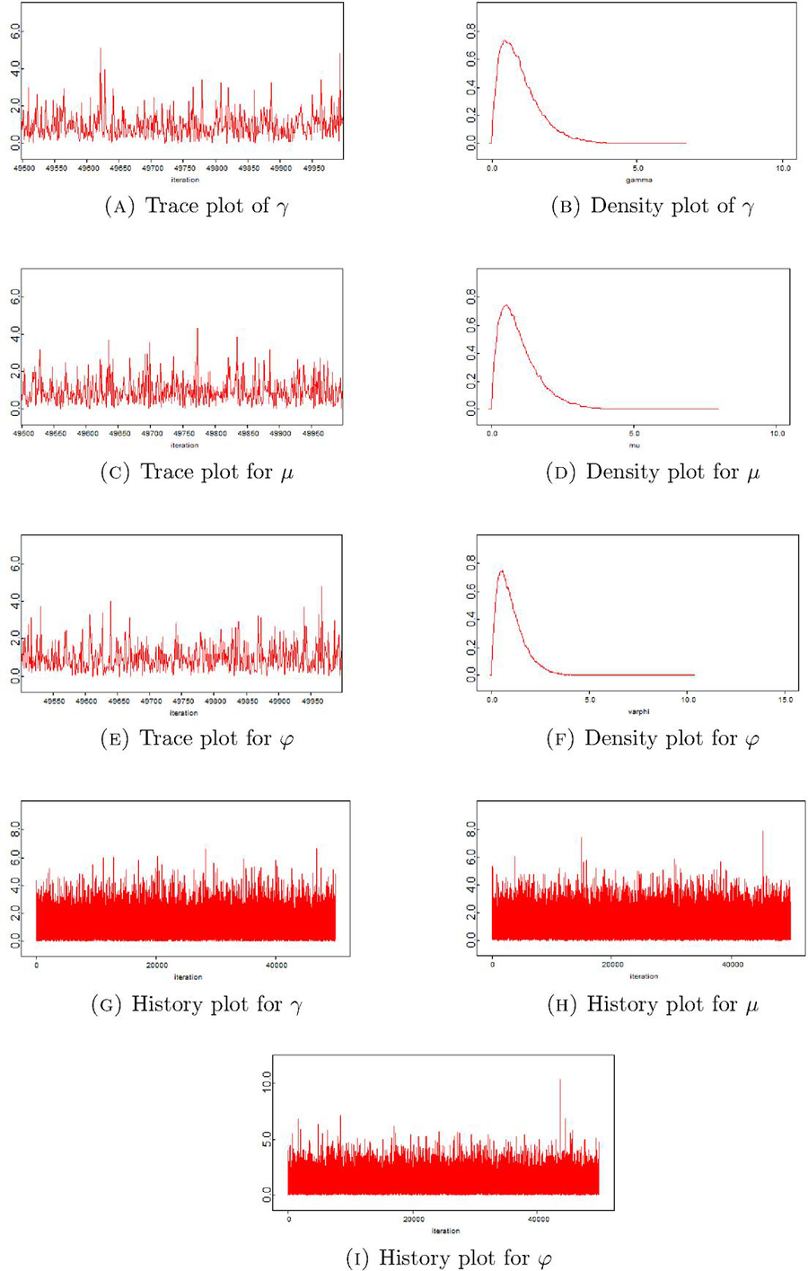
Figure 2 Trace, density and history plots for simulated data.

Modern Bayesian analysis is heavily dependent on the Markov Chain Monte Carlo (MCMC) methods, which make this approach very flexible. In the past, solving complex integration to have an analytical answer was a major problem in Bayesian studies. Since the Bayes estimators cannot be obtained in closed form, we use a Metropolis-Hasting approach to compute the posterior summaries. Metropolis-Hasting is a powerful MCMC approach that does not depends on the conditional distribution compared to the Gibbs sampling. In particular, informative prior with the hyperparameters $a=b=c=2$ and $d=e=f=2$, which result into $\text{mean}=1$ and $\text{variance}=0.5$, is used for the parameters $\gamma ,\mu$ and $\phi$. The Bayes estimates are calculated using the SELF and results are tabulated in Table 2. To asses the convergence of the process, we also use graphical diagnostics, like trace, density, and history plots of MCMC which are plotted in Figure 2. The trace plot are depicted in Figure 2 for each of the parameters of the ECD to show the behavior of different sampled values over time. The density plots reflect the fact that the MH algorithm uses the proposal distribution to generate a mixture distribution. History plot gives the detailed view of the trace plot for each parameter. In our study, one can see from a graphical assessment that the chains converge quite well.

Table 2 Posterior summaries using informative prior

n	Node	Mean	SD	MC Error	2.5%	Median	97.5%
10	$\gamma$	1.005	0.7078	0.00745	0.1191	0.8414	2.739
	$\mu$	1.012	0.7124	0.00658	0.1262	0.8479	2.837
	$\phi$	1.002	0.7149	0.00671	0.1186	0.8506	2.746
20	$\gamma$	1.006	0.7093	0.00512	0.1222	0.8474	2.791
	$\mu$	1.008	0.7150	0.00491	0.1204	0.8425	2.827
	$\phi$	0.999	0.7111	0.00453	0.1211	0.8456	2.747
30	$\gamma$	1.003	0.7082	0.00412	0.1209	0.8470	2.768
	$\mu$	1.004	0.7134	0.00419	0.1213	0.8369	2.824
	$\phi$	1.003	0.7128	0.00401	0.1213	0.8431	2.768
40	$\gamma$	1.001	0.7067	0.00369	0.1218	0.8446	2.771
	$\mu$	1.005	0.7163	0.00361	0.1207	0.8374	2.838
	$\phi$	1.003	0.7132	0.00348	0.1211	0.8424	2.777
50	$\gamma$	0.997	0.7044	0.00329	0.1206	0.8421	2.767
	$\mu$	1.002	0.7134	0.00325	0.1201	0.8357	2.822
	$\phi$	1.004	0.7146	0.00302	0.1213	0.8416	2.784

Table 3 Posterior summaries using non-informative priors

n	Node	Mean	SD	MC Error	2.5%	Median	97.5%
10	$\gamma$	1.344	1.337	0.01353	0.0325	0.9290	4.876
	$\mu$	1.332	1.304	0.01167	0.0347	0.9412	4.809
	$\phi$	1.332	1.332	0.01307	0.0332	0.9159	4.914
20	$\gamma$	1.335	1.333	0.01023	0.0342	0.9213	4.857
	$\mu$	1.330	1.319	0.00817	0.0337	0.9351	4.903
	$\phi$	1.334	1.332	0.00914	0.0342	0.9218	4.920
30	$\gamma$	1.324	1.321	0.00745	0.0347	0.9167	4.808
	$\mu$	1.335	1.326	0.00737	0.0330	0.9346	4.924
	$\phi$	1.341	1.337	0.00773	0.0337	0.9304	4.933
40	$\gamma$	1.323	1.321	0.00698	0.0339	0.9124	4.822
	$\mu$	1.335	1.329	0.00590	0.0329	0.9339	4.938
	$\phi$	1.344	1.338	0.00613	0.0338	0.9331	4.954
50	$\gamma$	1.320	1.317	0.00606	0.0344	0.9122	4.814
	$\mu$	1.335	1.327	0.00551	0.0330	0.9324	4.949
	$\phi$	1.343	1.335	0.00548	0.0338	0.9314	4.952

To assess the effect of noninformative priors, the Bayes estimates are also computed using $a=c=1$ and $b=d=0.75$, which result into $mean=1.33$ and $variance=1.78$. It is noticed that the results obtained by using the non-informative prior, Table 3, are different than the informative prior case, Table 2, in the sense of higher standard error and MC error. As discussed in the previous section that proper assessment of prior sensitivity is very important, we re-computed the Bayes estimates assuming different hyperparameters values. The results are listed in Table 4 where the first row represents the Bayes estimates using hyperparameters that results 0.5 variance. Similarly, the other hyperparameters used in this study are listed in the first cell of each row of Table 4. To discuss results more precisely, we restrict our discussion to two cases, that is, informative versus non-informative prior. It can be seen from rows 2–4 of the table that if the variance is between 0.5 and 1, the Bayes estimates are approximately the same whereas the standard errors are slightly high. However, rows 5–6 indicate that when the variance of the prior distribution exceeds 1, the Bayes estimates are noticed larger than the prefixed nominal values and the standard errors are also quite large. Thus, it is concluded that the first case is less sensitive because the change in the priors from row 2–4 does not make any significant difference as compared to the results of row 1. Contrary to this, the second case is more sensitive, as the priors used in the last two rows produce different results than the rest.

Table 4 Sensitivity analysis using different priors

Prior	Mean	SD	MC Error	2.5%	Median	97.5%
$\gamma$(2,2)	0.997	0.7044	0.00329	0.1206	0.8421	2.767
$\mu$(2,2)	1.002	0.7134	0.00325	0.1201	0.8357	2.822
$\phi$(2,2)	1.004	0.7146	0.00302	0.1213	0.8416	2.784
$\gamma$(1.5,1.5)	1.001	0.7594	0.00341	0.0939	0.817	2.950
$\mu$(1.5,1.5)	1.004	0.7635	0.00337	0.0957	0.8212	2.961
$\phi$(1.5,1.5)	1.002	0.7576	0.00324	0.0987	0.8198	2.938
$\gamma$(1.2,1.2)	1.002	0.9165	0.00377	0.0417	0.7386	3.446
$\mu$(1.2,1.2)	1.004	0.9124	0.00417	0.0442	0.7475	3.400
$\phi$(1.2,1.2)	1.004	0.9209	0.00369	0.0449	0.7438	3.439
$\gamma$(1,1)	0.989	0.9877	0.00454	0.0258	0.6841	3.611
$\mu$(1,1)	1.001	0.9955	0.00413	0.0248	0.6993	3.712
$\phi$(1,1)	1.007	1.0010	0.00411	0.0253	0.6985	3.714
$\gamma$(1,0.75)	1.320	1.3170	0.00606	0.0344	0.9122	4.814
$\mu$(1,0.75)	1.335	1.3271	0.00551	0.0330	0.9324	4.949
$\phi$(1,0.75)	1.343	1.3350	0.00548	0.0338	0.9314	4.952
$\gamma$(2,1)	1.995	1.4091	0.00658	0.2412	1.6840	5.534
$\mu$(2,1)	2.004	1.4270	0.00650	0.2401	1.6711	5.645
$\phi$(2,1)	2.008	1.4290	0.00605	0.2427	1.6830	5.567

To obtain the prediction of a future record value under the methods discussed in Section 5, 50 random observations of upper record values are generated from the ECD with $\gamma =\mu =\phi =1$. The generated observations are given below.

0.002274756, 0.006270403, 0.045944343, 0.051727181, 0.058437952,
0.063922531, 0.101346749, 0.108894021, 0.111617942, 0.146417615,
0.189417577, 0.192859033, 0.210283739, 0.231513991, 0.268381071,
0.270724046, 0.294144448, 0.332739834, 0.359738550, 0.365599712,
0.381377851, 0.394667327, 0.401582031, 0.409507793, 0.453030212,
0.458217009, 0.459556415, 0.470093353, 0.476450090, 0.494024277,
0.536271210, 0.569521517, 0.614420238, 0.620284956, 0.627418804,
0.636715619, 0.637374831, 0.655008180, 0.656443801, 0.667602313,
0.673574564, 0.675018108, 0.675135805, 0.680501538, 0.681368387,
0.695071138, 0.711500379, 0.716533342, 0.726979873, 0.728704883.

Since the goal is to predict 51st record value on the basis of generated 50 upper record observations, we use $a=b=c=2$, and $d=e=f=2$ as the hyperparameter values. The Bayesian future prediction is 1.796 while the conditional median prediction is 1.421. The $95\%$ Bayesian predictive interval for the future record is $(0.1048-5.5780)$.

7 Real Data Analysis

A real data set taken from Lawless (2011) to illustrate the proposed methodology. The data set comprises of 24 observations, 0.014, 0.034, 0.059, 0.061, 0.069, 0.08, 0.123, 0.142, 0.165, 0.21, 0.381, 0.464, 0.479, 0.556, 0.574, 0.839, 0.917, 0.969, 0.991, 1.064, 1.088, 1.091, 1.174, 1.27, which represents the quantity of 1000s of cycles to failure for electrical appliances in a life test.

To assess the goodness of fit of the ECD and select appropriate model, we compare ECD with two parameter Chen, Weibull, exponential and generalized exponential distributions using the real data set. For model selection and goodness of fit assessment, we used Akaike Information Criterion (AIC), Bayesian Information Criterion (BIC), Kolmogorov-Smirnov (KS) statistic, Cramer-von Mises (CVM) statistic and Anderson-Darling (AD) statistic. It is noticed that among the mentioned distributions, Exponentiated Chen is a decent contender to fit this data set as the least value of all information criteria is observed in the case of ECD.

Table 5 Model selection for the real data

Goodness-of-fit	ExpChen	Chen	Weibull	Exp	G Exp
AIC	13.60546	19.26221	21.84817	19.87926	21.86240
BIC	17.13962	21.61831	24.20428	21.05731	24.21850
KS	0.126029	0.155553	0.167998	0.167247	0.166566
CVM	0.060910	0.135710	0.145850	0.138593	0.133706
AD	0.381488	0.871534	0.917504	0.861168	0.826501

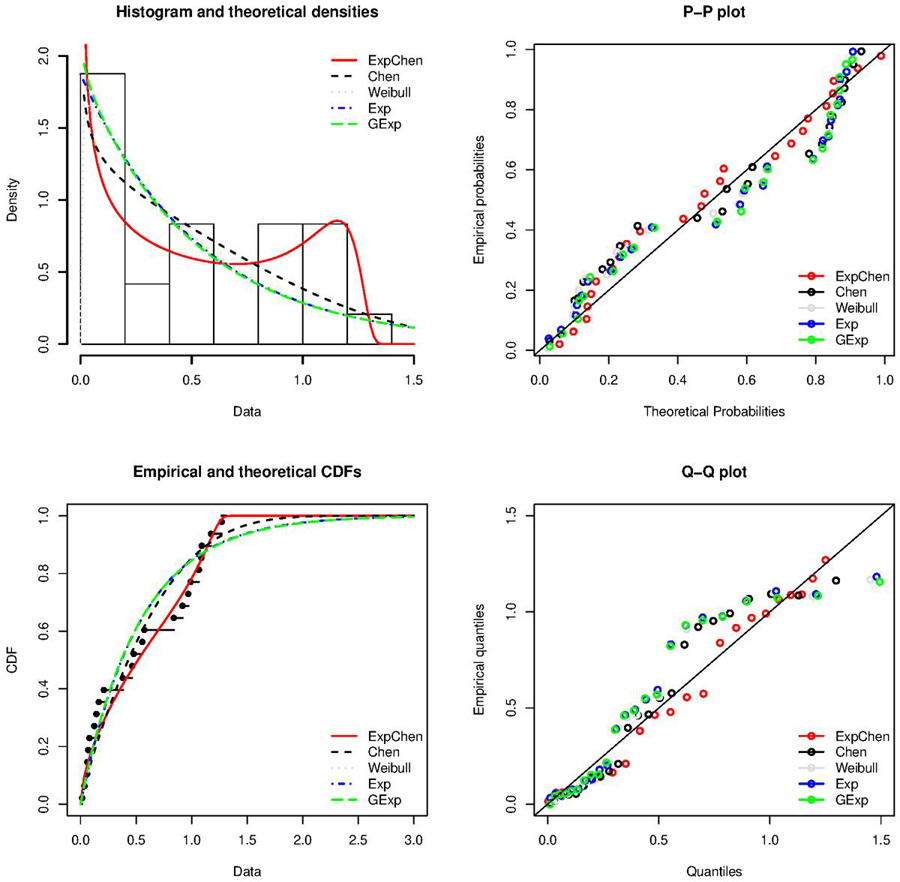
Figure 3 Visual goodness of fit assessment.

Table 6 Estimates for $\gamma ,\mu$ and $\phi$ based on real data

Parameter	MLE	BIP	BNIP
$\gamma$	1.2643	0.99771	1.32001
	(2.8127)	(0.70441)	(1.31701)
$\mu$	02127	1.00210	1.33511
	(0.0036)	(0.71342)	(1.32702)
$\phi$	1.0740	1.00402	1.34300
	(0.1480)	(0.71460)	(1.33513)

The frequentist and Bayes estimates are listed in Table 5. For the Bayesian case, SELF is used to compute the Bayes estimates assuming informative and non-informative priors. To be more specific, independent gamma priors with with hyperparameters $a=b=c=d=e=f=2$ and $a=c=e=1,b=d=f=0.75$ to have informative and non-informative priors are considered. In the table, the abbreviations MLE, BIP, and BNIP are used for the maximum likelihood estimates, Bayes estimates using informative prior and Bayes estimates using non-informative prior, respectively.

The credible intervals for $\gamma$, $\mu$ and $\phi$ are $(0.1191,2.739)$, $(0.1262,2.837)$ and $(0.1186,2.746)$, respectively. Similarly, the predicted future record value is 1.954 while the conditional median prediction is 1.696. The 95% Bayesian predictive interval for the future record value is $(0.09344,4.4331)$. Thus, both the future prediction and the future conditional median fall within the 95% Bayesian interval. In addition, the graphical diagnostics using the Trace, Density and History plots are depicted in Figure 4. It is worth mentioning that the trace plots of each parameter of the ECD tell about the values that the parameter took during the runtime of the chain.

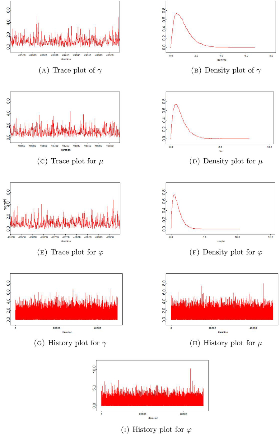
Figure 4 Trace, density and history plots for real data.

8 Conclusion

This study discussed the statistical inference for the three-parameter exponentiated Chen distribution based on upper record values. The reason of considering this positively skewed distribution is its flexibility in terms of bathtub-shaped hazard rate. Bayesian and frequentist methods are used to obtain the point estimates as well as the two-sided confidence intervals. To be more specific, the Bayes estimates are computed by using informative and non-informative priors, where independent gamma priors are assumed for the scale and the shape parameters. As the Bayes and ML estimators cannot be solved analytically, Newton Raphson and MCMC procedure are used to calculate the MLE and Bayes estimators. To evaluate the impact of hyperparameters, a sensitivity analysis is also presented in this article. In addition, two different methods for generating record values are presented in this study. A simulation study as well as a real data set is used to assess the efficiency of the numerical methods. For the real data set, the model selection is done using AIC, BIC, KS, CVM and AD measures. The results suggest that the exponentiated Chen distribution performs better than the other competitive lifetime distributions. In the future, this work can be extended by using the lower record values.

References

Abdi and Asgharzadeh (2018) Abdi, M. and Asgharzadeh, A. (2018). Rayleigh confidence regions based on record data. Journal of Statistical Research of Iran, 14(2):171–188.

Ahmadi et al. (2009) Ahmadi, J., Jozani, M. J., Marchand, É., and Parsian, A. (2009). Prediction of k-records from a general class of distributions under balanced type loss functions. Metrika, 70(1):19–33.

Ahsanullah (1995) Ahsanullah, M. (1995). Record Statistics. Nova Science Publishers.

Ahsanullah and Nevzorov (2015) Ahsanullah, M. and Nevzorov, V. B. (2015). Records via Probability Theory. Springer.

Al-Duais (2021) Al-Duais, F. S. (2021). Bayesian analysis of record statistic from the inverse Weibull distribution under balanced loss function. Mathematical Problems in Engineering, 2021(15):1–9.

Al-Hussaini and Ahmad (2003) Al-Hussaini, E. K. and Ahmad, A. E.-B. A. (2003). On Bayesian interval prediction of future records. Test, 12(1):79–99.

Alhamidah et al. (2023) Alhamidah, A., Qmi, M. N., and Kiapour, A. (2023). Comparison of E-Bayesian estimators in Burr XII model using E-PMSE based on record values. Statistics, Optimization & Information Computing, 1:709–718.

Arnold et al. (2011) Arnold, B. C., Balakrishnan, N., and Nagaraja, H. N. (2011). Records, volume 768. John Wiley & Sons.

Arshad and Jamal (2019) Arshad, M. and Jamal, Q. A. (2019). Estimation of common scale parameter of several heterogeneous Pareto populations based on records. Iranian Journal of Science and Technology, Transactions A: Science, 43:2315–2323.

Awodutire (2022) Awodutire, P. O. (2022). Statistical properties and applications of the exponentiated Chen-G family of distributions: Exponential distribution as a baseline distribution. Austrian Journal of Statistics, 51(2):57–90.

Azimi et al. (2023) Azimi, R., Esmailian, M., and Gallardo, D. (2023). The inverted exponentiated Chen distribution with application to cancer data. Japanese Journal of Statistics and Data Science, 6:213–241.

Basak and Balakrishnan (2003) Basak, P. and Balakrishnan, N. (2003). Maximum likelihood prediction of future record statistic. In Mathematical and Statistical Methods in Reliability, pages 159–175. World Scientific.

Chandler (1952) Chandler, K. N. (1952). The distribution and frequency of record values. Journal of the Royal Statistical Society, Series B (Methodological), 14(2):220–228.

Chaubey and Zhang (2015) Chaubey, Y. P. and Zhang, R. (2015). An extension of Chen’s family of survival distributions with bathtub shape or increasing hazard rate function. Communications in Statistics-Theory and Methods, 44(19):4049–4064.

Chen (2000) Chen, Z. (2000). A new two-parameter lifetime distribution with bathtub shape or increasing failure rate function. Statistics & Probability Letters, 49(2):155–161.

Dey et al. (2017) Dey, S., Kumar, D., Ramos, P. L., and Louzada, F. (2017). Exponentiated Chen distribution: Properties and estimation. Communications in Statistics-Simulation and Computation, 46(10):8118–8139.

Dziubdziela and Kopociński (1976) Dziubdziela, W. and Kopociński, B. (1976). Limiting properties of the k-th record values. Applicationes Mathematicae, 2(15):187–190.

El-Din et al. (2015) El-Din, M. M., Abdel-Aty, Y., Shafay, A., and Nagy, M. (2015). Bayesian inference for the left truncated exponential distribution based on ordered pooled sample of records. Journal of Statistics Applications & Probability, 4(1):1–11.

Eliwa et al. (2021) Eliwa, M. S., El-Morshedy, M., and Ali, S. (2021). Exponentiated odd Chen-G family of distributions: Statistical properties, Bayesian and non-Bayesian estimation with applications. Journal of Applied Statistics, 48(11):1948–1974.

Hastings (1970) Hastings, W. K. (1970). Monte carlo sampling methods using markov chains and their applications. Biometrika, 57(1):97–197.

Hjorth (1980) Hjorth, U. (1980). A reliability distribution with increasing, decreasing, constant and bathtub-shaped failure rates. Technometrics, 22(1):99–107.

Khan et al. (2016) Khan, M. S., King, R., and Hudson, I. L. (2016). Transmuted exponentiated Chen distribution with application to survival data. ANZIAM Journal, 57:268–290.

Khan et al. (2018) Khan, M. S., King, R., and Hudson, I. L. (2018). Kumaraswamy exponentiated Chen distribution for modelling lifetime data. Applied Mathematics & Information Sciences, 12(3):617–623.

Kumar and Gupta (2023) Kumar, R. and Gupta, R. (2023). Bayesian analysis of inverse Rayleigh distribution under non-informative prior for different loss functions. Thailand Statistician, 21(1):76–92.

Lawless (2011) Lawless, J. F. (2011). Statistical Models and methods for lifetime data, volume 362. John Wiley & Sons.

Madi and Raqab (2004) Madi, M. T. and Raqab, M. Z. (2004). Bayesian prediction of temperature records using the pareto model. Environmetrics, 15(7):701–710.

Martz and Waller (1982) Martz, H. and Waller, R. (1982). Bayesian Reliability Analysis. John Wiley & Sons, Inc.

Metropolis et al. (1953) Metropolis, N., Rosenbluth, A. W., Rosenbluth, M. N., Teller, A. H., and Teller, E. (1953). Equation of state calculations by fast computing machines. The Journal of Chemical Physics, 21(6):1087–1092.

Mousa et al. (2002) Mousa, M. A., Jaheen, Z., and Ahmad, A. (2002). Bayesian estimation, prediction and characterization for the gumbel model based on records. Statistics: A Journal of Theoretical and Applied Statistics, 36(1):65–74.

Méndez-González et al. (2023) Méndez-González, L. C., Rodríguez-Picón, L. A., Pérez-Olguín, I. J. C., and Vidal Portilla, L. R. (2023). An additive Chen distribution with applications to lifetime data. Axioms, 12(2).

Nagaraja (1977) Nagaraja, H. (1977). On a characterization based on record values. Australian Journal of Statistics, 19(1):70–73.

Nevzorov (1988) Nevzorov, V. B. (1988). Records. Theory of Probability & Its Applications, 32(2):201–228.

Pak et al. (2022) Pak, A., Raqab, M., Mahmoudi, M. R., Band, S. S., and Mosavi, A. (2022). Estimation of stress-strength reliability $r=p(x>y)$ based on Weibull record data in the presence of inter-record times. Alexandria Engineering Journal, 61(3):2130–2144.

Pakhteev and Stepanov (2016) Pakhteev, A. and Stepanov, A. (2016). Simulation of gamma records. Statistics & Probability Letters, 119:204–212.

Rajarshi and Rajarshi (1988) Rajarshi, S. and Rajarshi, M. (1988). Bathtub distributions: A review. Communications in Statistics-Theory and Methods, 17(8):2597–2621.

Seo and Kim (2017) Seo, J. I. and Kim, Y. (2017). Objective Bayesian analysis based on upper record values from two-parameter Rayleigh distribution with partial information. Journal of Applied Statistics, 44(12):2222–2237.

Soliman and Al-Aboud (2008) Soliman, A. A. and Al-Aboud, F. M. (2008). Bayesian inference using record values from Rayleigh model with application. European Journal of Operational Research, 185(2):659–672.

Srivastava (1979) Srivastava, R. (1979). Two characterizations of the geometric distribution by record values. Sankhyā: The Indian Journal of Statistics, Series B, 40(3):276–278.

Xie and Lai (1996) Xie, M. and Lai, C. D. (1996). Reliability analysis using an additive Weibull model with bathtub-shaped failure rate function. Reliability Engineering & System Safety, 52(1):87–93.

Xie et al. (2002) Xie, M., Tang, Y., and Goh, T. N. (2002). A modified Weibull extension with bathtub-shaped failure rate function. Reliability Engineering & System Safety, 76(3):279–285.

Yousaf et al. (2019) Yousaf, F., Ali, S., and Shah, I. (2019). Statistical inference for the Chen distribution based on upper record values. Annals of Data Science, 6: 831–853.

Biographies

Farhad Yousaf is currently pursuing his PhD statistics from University of Naples Federico II, Naples, Italy. Prior to this he completed his MPhil in Statistics from Department of Statistics, Quaid-i-Azam University, Islamabad, Pakistan. His research interest is focused on Bayesian inference, socia network analysis, and data science.

Sajid Ali is Associate Professor at the Department of Statistics, Quaid-i-Azam University (QAU), Islamabad, Pakistan. He graduated (PhD Statistics) from Bocconi University, Milan, Italy. His research interest is focused on Bayesian inference, construction of new flexible probability distributions, electricity market modeling, and process monitoring.

Ismail Shah is currently serving as a researcher at the university of Padua. He is also an Associate Professor with the Department of Statistics, Quaid-i-Azam University, Islamabad, Pakistan. He received PhD degree in Statistics from University of Padova, Italy. His research interest areas are: Functional Data Analysis, Time Series Modeling, Electricity Market Modeling and Applied Statistics. Currently, he is also the editor of Journal of Quantitative Methods https://ojs.umt.edu.pk/index.php/jqm.

Saba Riaz is currently an assistant professor at Department of statistics, Rawalpindi Women University. She completed her PhD in Statistics from Quaid-i-Azam University (QAU), Islamabad, Pakistan. Her research interests are: survey sampling, and applied statistics.

Journal of Reliability and Statistical Studies, Vol. 16, Issue 1 (2023), 197–228.
doi: 10.13052/jrss0974-8024.16110
© 2023 River Publishers