System Reliability Analysis of Large Capacity Electric Mining Trucks Used in Coal Mining

Sedat Toraman

Turkey Directorate General of Coal Enterprises, Yenimahalle, Turkey
E-mail: sedat.toraman@gmail.com

Received 07 March 2023; Accepted 23 June 2023; Publication 06 July 2023

Abstract

In today’s world where competition is increasing, the focus of all efforts on meeting production targets at the lowest possible cost has increased the need for maximum benefit from existing machinery/equipment. In this context, availability, reliability and maintainability analysis have become the basic tools to be used in meeting this need.

In this study, reliability, maintainability and availability values were determined using the operation and repair data (2019) of large capacity electric trucks used in the Manisa-Soma coal field. First of all, each truck was analyzed and then the analysis of the entire truck system was performed. In this context, RAM analysis of all trucks was performed and then the general reliability of the entire truck system was calculated by considering the working order in the enterprise. According to this; The truck with the highest reliability is the truck with door number 555 and the reliability rate is 77.04%, and the truck with the lowest reliability is the truck number 556 with a rate of 26.31%. As a result of the maintainability analysis, the truck with the 553 door number had the highest maintainability with a rate of 73.52%. The truck numbered 549 has the lowest maintainability rate with a rate of 42.21%. As a result of the system analysis, the reliability rate was determined as 24% in R (1000) minutes, 59% in R (500) minutes and 83% in R (250) minutes.

Keywords: Electric mining truck, ram analysis, reliability, maintainability, availability.

1 Introduction

Availability, which is a widely used criterion in planning maintenance and production activities, refers to the possibility of a machine to operate at a satisfactory level when needed. With the increase in availability, the time spent by the machine in production will increase and the cost of lost time will decrease accordingly. Availability, also known as usage rate, is a concept that combines both reliability and maintainability. Reliability refers to the possibility of a machine working in a certain time period, while ease of maintenance refers to the possibility of making a machine that fails operational again in a certain time interval [1].

The reliability of a machine may not be high, but if it can be repaired quickly when it fails, its availability will be high. Therefore, while it is important for a machine to remain operational, it is desirable that the maintenance of the machine is easy, fast and within a reasonable cost range.

A production activity consists of different types of machinery and equipment, each of which is used to perform specific activities, and mostly operates as a serially connected system. The reliability of such a system depends on the functioning of all its subsystems. Maintenance is defined as all of the operations and activities performed to prevent or control unexpected malfunctions and possible stops as much as possible [2]. As such, it plays a key role in production activities due to its effect on the ability to carry out production according to plans by increasing system reliability.

The statistical evaluation of the failure results of the machines, each of which has its own different failure behavior and service requirements, plays an important role in the proper performance of the maintenance function. At this stage, how often a machine malfunctions and how long it takes to work again should be evaluated according to the criteria of “Reliability, Availability and Maintainability” (“RAM”). Thus, it will be possible to create maintenance plans for each machine in accordance with its own conditions.

Understanding the positive contribution of being present on production activities has led to an increase in the work done in this field. In this context, efforts to collect and analyze maintenance data to calculate reliability, availability and ease of maintenance have increased significantly in recent years. Reliability is the probability of an object to fully fulfill a defined purpose within a certain time frame [3, 4]. With the rise of modern technology in the last fifty years, the concept of reliability has gained more importance. The science of statistics, which is widely used in many fields, has gained an important place in reliability analysis with its probability distributions.

In reliability analysis, discrete distributions from probability distributions deal with discrete events such as the number of errors occurring in a certain time interval. Continuous distributions are used to model variables that take any value, such as duration versus time [5].

Probability distributions are widely used as corruption versus time or failure models for systems, subsystems or components [3, 6]. The lifetime of a system; amount of production depends on many factors such as, the material used for production or the change in environmental conditions. First, the system or a subsystem of the system or a component of the system is taken as a random variable and a suitable probability model is created for deterioration or failure against time. Then the parameters in the created probability model are estimated. In addition, some features of the created probability models such as survival function and hazard function are examined [7].

For reliability and maintainability calculations, the analysis should be started by determining which distribution system the data is suitable for. After a researcher determines which distribution the data fits into, it can easily analyze by using the characteristics of this distribution. Data showing the lifetime of units such as electronic and mechanical devices, people, information processing systems and many other systems generally have the feature of continuous random variables. Therefore, the lifetime distributions of such data are also continuous distributions. The important continuous distributions to which these data are widely matched; Normal, Log-normal, Exponential, Weibull, Erlang, Gamma and Rayleigh distributions [8].

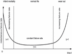
The probability distribution with the most common use in reliability studies is the Weibull distribution [9]. The Weibull distribution has the ability to characterize all phases of the bathtub characteristic curve (Figure 1) called the adjustment period, useful life period and wear period and all behaviors of the curve.

Zone 1 covers the time when early damage occurs, damage gradually decreases. Types of faults in this area can be assembly errors, manufacturing defects, material defects and open construction faults.

Zone 2 is the zone where accidental damages occur, the damages are fixed or closely followed by the constant. Usage error or lack of maintenance may cause this type of malfunction.

Zone 3 is the area where wear and fatigue damages occur, the damages gradually increase. Examples such as fatigue fracture, aging, and tingling can be given.

Figure 1 Bathtub characteristic curve [9].

In order to understand and predict the failure characteristics of a machine, Reliability, Availability and Maintainability – RAM analysis is required. The basic equations related to these criteria are listed in Table 1.

Table 1 Basic equations [2]

$R(t)=P(T>t)=1-P(t\le t)$	$M(t)=P(T\le t)={\displaystyle {\int }_0^t}f(t).dt$
$R(t)=1-{\displaystyle {\int }_0^t}f(t).dt\to R(t)$ $={\displaystyle {\int }_t^{\mathrm{\infty }}}f(t).dt$	$\mathit{MTTF}={\displaystyle {\int }_t^{\mathrm{\infty }}}t.f(t).dt$ $={\displaystyle {\int }_t^{\mathrm{\infty }}}[1-M(t)].dt$
$\mathit{MTBF}={\displaystyle {\int }_t^{\mathrm{\infty }}}t.f(t).dt$ $={\displaystyle {\int }_t^{\mathrm{\infty }}}[1-F(t)].dt$ $={\displaystyle {\int }_t^{\mathrm{\infty }}}R(t).dt$	T $\mathrm{=}$ Repair time(continuous random variable) M(t) $\mathrm{=}$ Maintainability MTTF $\mathrm{=}$ Mean time to failures
$\lambda ={\displaystyle \frac{f(t)}{R(t)}}$	Availability (A)
T $\mathrm{=}$ Repair time f(t) $\mathrm{=}$ Probability density function R(t) $\mathrm{=}$ Reliability F(t) $\mathrm{=}$ Cumulative density function MTBF $\mathrm{=}$ Mean time between failures $\lambda$ $=$ Failure rate	$A(t)=P\{X(t)=1\};t>0$ $A={\displaystyle \frac{\mathit{MTBF}}{\mathit{MTBF}+\mathit{MTTF}}}$ X(t) $\mathrm{=}$ The state of a system at time t (In working condition $X\mathrm{(}t\mathrm{)}\mathrm{=}\mathrm{1}\mathrm{)}$ (In case of failure $X\mathrm{(}t\mathrm{)}\mathrm{=}\mathrm{0}\mathrm{)}$

Mean time between failures (MTBF) is the predicted elapsed time between inherent failures of a mechanical or electronic system during normal system operation. MTBF can be calculated as the arithmetic mean (average) time between failures of a system [12].

Due to the effect of various factors on the time to failure and the downtime/downtime, these times can take a random value and have the characteristics of a continuous random variable. Failure distributions define the time a system spends until it fails, while repair distributions define the time required for the repair of a failed system. The only difference between the distributions is in how these methods are used. For example, the probability of deterioration gives the probability of failure at a certain time, while reliability gives the probability of failure to occur. In the case of repair distributions, the probability of an event occurring (repair of the part) is dealt with, as is the probability of deterioration. When making calculations in RAM analysis, it is important to determine which probability distribution the failure and repair times are appropriate. Common distributions for breakdown and repair times are Weibull, Lognormal, normal and exponential distributions, and the basic equations related to these distributions are given below (Table 2).

Table 2 Breakdown and repair distributions [10]

	Exponential	Lognormal	Normal	Weibull
$f(t)*$	$=\lambda e^{-\lambda t}$	$={\displaystyle \frac{1}{\sigma \sqrt{2\pi }}}{e}^{{\displaystyle \frac{{(lnt-\mu )}^2}{2{\sigma }^2}}}$	$={\displaystyle \frac{1}{\sigma \sqrt{2\pi }}}{e}^{{\displaystyle \frac{{(t-\mu )}^2}{2{\sigma }^2}}}$	$=\beta {\alpha }^{-\beta }{t}^{\beta -1}{e}^{{(t/\alpha )}^{\beta }}$
$\mathit{MTBF}$	$=1/\lambda$	$=e^{{\displaystyle \frac{\mu +{\sigma }^2}{2}}}$	$=\mu$	$=\alpha \mathrm{\Gamma }{\left(1+{\displaystyle \frac{1}{\beta }}\right)}^{**}$
$\mathit{MTTF}$	$=1/\lambda$	$=e^{{\displaystyle \frac{\mu +{\sigma }^2}{2}}}$	$=\mu$	$=\alpha \mathrm{\Gamma }\left(1+{\displaystyle \frac{1}{\beta }}\right)$
$R(t)$	$e^{-\lambda t}$	$=1-\mathrm{\Phi }{\left({\displaystyle \frac{lnt-\mu }{\sigma }}\right)}^{***}$	$=1-\mathrm{\Phi }\left({\displaystyle \frac{t-\mu }{\sigma }}\right)$	$=e^{-{({\displaystyle \frac{t}{\alpha }})}^{\beta }}$
$M(t)$	$=1-e^{-\lambda t}$	$=\left({\displaystyle \frac{lnt-\mu }{\sigma }}\right)$	$=\mathrm{\Phi }\left({\displaystyle \frac{t-\mu }{\sigma }}\right)$	$=1-e^{-{({\displaystyle \frac{t}{\alpha }})}^{\beta }}$
*Probability density function **$\mathrm{\Gamma }$ $\mathrm{=}$ Gamma function ***$\mathrm{\Phi }$ $\mathrm{=}$ Cumulative distribution function.

2 Analysis of Electric Trucks Used in Manisa-Soma Open Pit Mining

Efficient operation of mining machines (excavators, trucks, etc.), which are purchased and operated with great investment values, is very important in terms of cost factors. For this purpose, it is very important for an effective study to perform reliability, maintenance and availability RAM analysis of machines and equipment in certain periods (6 months to 1 year).

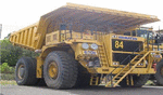
Figure 2 630S electric truck

In this study, the data of electric trucks (170 Ston) operating in the Manisa-Soma coal field were used. A total of 10 Komatsu 630ES trucks in the establishment have increased their breakdown frequency due to their long-term operation, and thus their utilization rates have decreased. It has become necessary to carry out reliability, maintenance and availability analysis of electric trucks, which directly and largely affect costs.

Operation times and downtimes of trucks were obtained from the recording systems available in the enterprise. Considering that the establisment works in 2 shifts, it is seen that it works 16 hours a day and therefore the working times between failures were evaluated over 16 hours. Repair times, on the other hand, were evaluated over 8 hours per day, since the work was carried out in one shift per day.

Table 3 Failures and repair times of trucks

		Total Number	Total Repair	Average Failure
Truck No	Data Range	of Failures	Time (h)	Repair Time (h)
548	01.03.2019–31.10.2019	84	387	4.60
549	01.03.2019–31.10.2019	73	145	1.98
550	01.03.2019–31.10.2019	125	263	2.10
551	01.03.2019–31.10.2019	68	147	2.16
552	01.03.2019–31.10.2019	121	274	2.26
553	01.03.2019–19.06.2019	103	203	1.97
554	01.03.2019–26.07.2019	94	134	1.42
555	01.03.2019–31.10.2019	67	225	3.35
556	20.06.2019–02.09.2019	85	336	3.95
557	01.03.2019–31.10.2019	85	191	2.24

When the Table 3 above is examined, it is seen that the electric truck with the most failure is the truck numbered 550 with 125 breakdowns and the truck with the least breakdown is the truck numbered 555 with 67 failure.

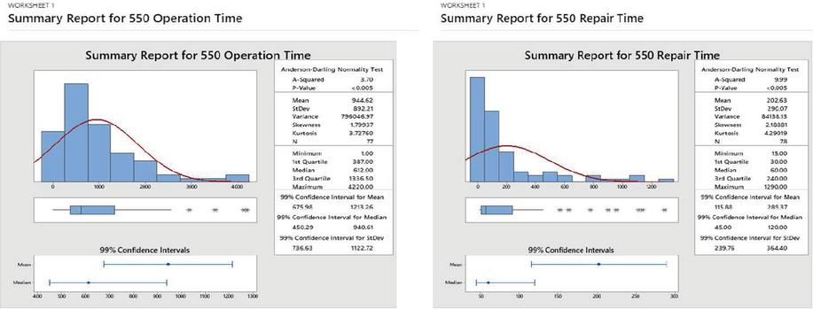
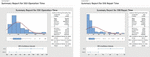
Figure 3 Summary Report for The Truck Number 550 (Minitab 19.1.1 version).

Mean time between failures (MTBF) describes the expected time between two failures for a repairable system in general, MTBF is the “up-time” between two failures states of a repairable system during operation as outlined here:

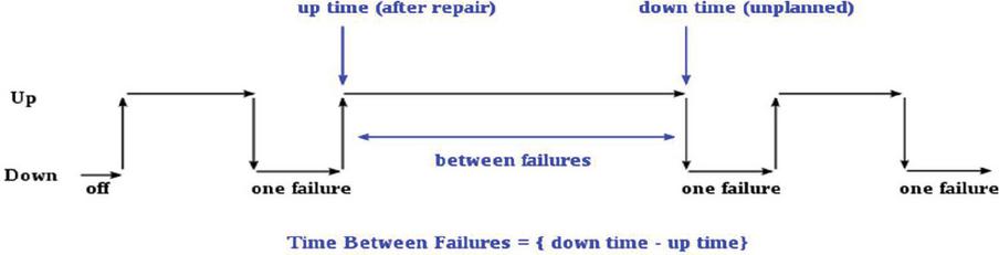
For each observation, the “down time” is the instantaneous time it went down, which is after (i.e. greater than) the moment it went up, the “up time”. The difference (“down time” minus “up time”) is the amount of time it was operating between these two events.

By referring to the figure above, the MTBF of a component is the sum of the lengths of the operational periods divided by the number of observed failures [12]:

$$\mathit{MTBF}=\frac{\sum (\mathit{Start}\mathit{of}\mathit{downtime}-\mathit{Start}\mathit{of}\mathit{uptime})}{\mathit{Number}\mathit{of}\mathit{failures}}$$

When the summary report of the truck numbered 550 (Figure 3) is examined, it is seen that the time between failures will be between 675 minutes (11.25 hours) and 1213 minutes (20 hours) with 99% reliability, and the repair time will be between 115 minutes and 289 minutes with 99% reliability. The mean time between failures (MTBF) was 1159 minutes, and the mean time to failure (MTTF) was 193 minutes. Summary report results for all trucks are detailed in the Table 4 below. When all trucks are examined, the truck that can operate for the longest time with 99% reliability is the truck number 555 with at least 1573 minutes, the truck that can be repaired in the shortest time is the truck number 553 with 0.59 minutes. Due to the metal fatigue and old age of the trucks, there are situations where MTBF values are greater than the operation values due to the high repair times rather than the operation time.

Table 4 MTBF and MTTF of trucks

	99% Confidence Operation	99% Confidence Repair
Truck No	Time (min.)	Time (min.)	MTBF	MTTF
548	761-1753	77-723	1691	329
549	1270-3344	99-326	2253	215
550	675-1213	115-289	1159	193
551	1121-2449	69-257	1888	129
552	1042-1733	114-330	1614	203
553	842-1757	10.59-273	1222	195
554	808-1978	36-329	1571	172
555	21573-3136	94-520	22355	303
556	260-1037	12-1331	1016	372
557	747-2349	81-361	1403	207

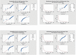
The time between failures data are only considered as the time the truck has been operating. Repair time is evaluated as the whole time between the time of entering the failure and the exit from the failure (if different types of failure occur consecutively on the same day, it is taken as a single failure period). Distribution analysis was carried out to determine with which distribution the 550 numbered truck time to failure (TTF) and time between failures(TBF) fit better (Figure 4). It was observed that the lognormal distribution was more suitable for TTF, and the TBF data were consistent with the Weibull distribution. All analyses were performed with Minitab 19.1.1.

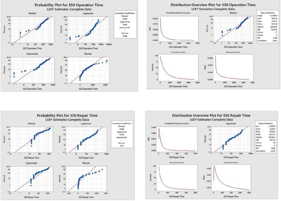
Figure 4 Plot Distribution analysis.

Distribution analysis have been made for all trucks and according to the analysis results, the parameters for both the time between failures (TBF) and time to failure (TTF) have been determined as follows (Table 5).

Table 5 Distribution analysis

Truck No		Distribution	Correlation	Parameters
548	TBF	Weibull	0.935	$\beta$: 0.642, $\eta$: 1222.94
	TTF	Lognormal	0.945	$\mu$: 4.751, $\sigma$:1.445
549	TBF	Weibull	0.989	$\beta$: 0.921, $\eta$: 2169.18
	TTF	Lognormal	0.978	$\mu$: 4.813, $\sigma$:1.058
550	TBF	Weibull	0.934	$\beta$: 0.778, $\eta$: 1003.63
	TTF	Lognormal	0.970	$\mu$: 4.509, $\sigma$:1.231
551	TBF	Weibull	0.982	$\beta$: 0.928, $\eta$: 1824.49
	TTF	Lognormal	0.909	$\mu$: 4.236, $\sigma$:1.122
552	TBF	Weibull	0.932	$\beta$: 0.913, $\eta$: 1546.96
	TTF	Lognormal	0.959	$\mu$: 4.440, $\sigma$:1.322
553	TBF	Weibull	0.930	$\beta$: 1.842, $\eta$: 1375.75
	TTF	Lognormal	0.908	$\mu$: 3.867, $\sigma$:1.174
554	TBF	Weibull	0.906	$\beta$: 0.884, $\eta$: 1478.49
	TTF	Lognormal	0.964	$\mu$: 4.405, $\sigma$:1.218
555	TBF	Normal	0.913	$\mu$: 2355.18, $\sigma$:1830.69
	TTF	Lognormal	0.967	$\mu$: 4.648, $\sigma$:1.461
556	TBF	Weibull	0.935	$\beta$: 0.544, $\eta$: 587.68
	TTF	Lognormal	0.925	$\mu$: 4.825, $\sigma$:1.478
557	TBF	Weibull	0.971	$\beta$: 0.974, $\eta$: 1387.33
	TTF	Lognormal	0.963	$\mu$: 4.498, $\sigma$:1.292

When the distribution characteristics of the data of the time between failures and the time to failure are examined, it is seen that the distribution of the working time data between failures is mostly suitable for the weibull distribution characteristics, and the time to failure data is suitable for the lognormal distribution.

After determining the parameters according to the distribution, Reliability R (t), Failure Probability F (t), Maintainability M (t) and Availability analyzes were performed for each truck to reveal the performance of individual trucks (Table 6).

Table 6 Reliability R (t), Failure Probability F (t), Maintainability M (t)

Truck No	Reliability R(1000 min.)	Maintainability M(100 dk)	Availability A %
548	41.53%	45.98%	83.71%
549	61.26%	42,21%	91.29%
550	36.89%	53.11%	85.72%
551	56.42%	62.89%	93.60%
552	51.10%	54.97%	88.83%
553	57.37%	73.52%	92.79%
554	49.28%	56.53%	90.13%
555	77.04%	48.83%	88.60%
556	26.31%	44.09%	73.20%
557	48.34%	53.31%	87.14%

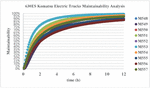
When the above table is examined, the reliability of the electric truck with door number 555 of the trucks with the highest reliability is 77%, and the reliability of the truck with door number 549 is 61%. The lowest performing truck with 26% reliability is the 556, while the other truck with the lowest performance is truck number 550. Reliability values of all trucks are given in Figure 5.

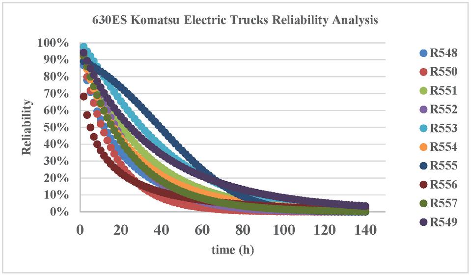
Figure 5 Reliability values of 10 electric Komatsu trucks.

The highest rate of maintainability within 100 minutes belongs to the truck numbered 553 with 73%. In terms of maintainability, truck number 553 is followed by truck number 551 with a ratio of 62%. Trucks with the lowest maintainability rates are 548, 556 and 549, respectively.

When the availability rates are examined, the truck numbered 551 has the highest rate with 93%. This truck is followed by the truck numbered 553 with 92%, 549 with 91% and 554 with 90%.

When the RAM analyzes are examined collectively, it is seen that the trucks 551, 553, 555, 549 have the best performance with high reliability, the maintainability and the availability rate. Truck with door number 556 It is the worst performing truck with lowest reliability, lowest maintainability and lowest availability.

When these data are examined, it is recommended that the company should primarily use the trucks 553, 555, 551 and 549, which have high reliability, and take care not to use the 556 numbered truck.

When Figure 5 is examined, the electric truck with the highest reliability is truck no. 555, and the truck with the lowest reliability is truck no. 556. The reliability of the truck no. 556 operating for 40 hours is 12%. On the other hand, the 40-hour operating reliability of the truck numbered 555 is 49%. The reliability of trucks 556, 550, 548, 554 is in the range of 0–5% for 100 hours.

Due to the fact that the trucks were purchased between 1998–2000, preventive and predictive maintenance studies were not carried out, and as a result of 20–25 years of operating performance, the reliability percentages are low.

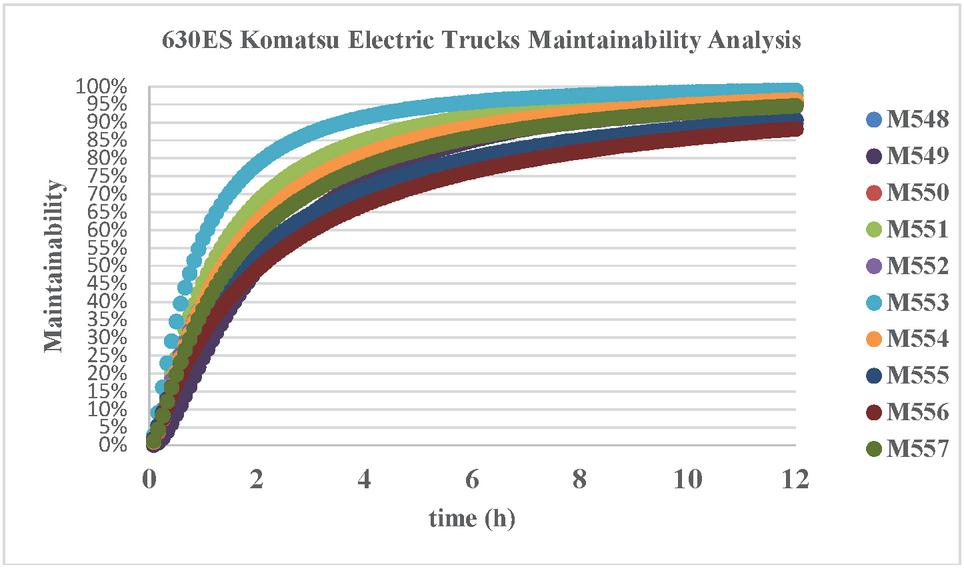
Figure 6 Maintainability behavior of electric Komatsu trucks.

Figure 6 shows the time-dependent change in ease of maintenance. Accordingly, the ease of maintenance of the truck no. 553 is quite high compared to other trucks. Secondly, the truck with the best ease of maintenance is truck number 551. Trucks 551, 552, 554 and 557 show similar repairability trends, while trucks 548, 555, 556 show similar ease of maintenance trends. The probability that the electric truck with door number 553 can be repaired within 2 hours is 80%. It is seen that 7.5 hours are required for the truck no. 556 to be repaired with 80% probability. If we were to rank from highest to lowest ease of maintenance, it would be 553, 551, 554, 552, 557, 550, 555, 548, 556, 549. With a 95% probability, it will take 5.5 hours for truck 553 to be repaired, while truck 551 will be repaired in 8.25 hours and truck 554 will take 10,167 hours. It takes more than 12 hours for other trucks to be repaired.

3 System Reliability

System structure is shown through reliability block diagram or structure function. This diagram and function reveals the relationship between the operating status or performance of the system and the operating conditions / performances of the components that make up the system. (Kuo ve Zuo, 2003:86). Systems according to the system structure; parallel, serial, parallel-serial, serial-parallel, bridged and so on. are classified as.

Reliability calculation in serial and parallel systems;

$\mathit{Rsystem}=R1xR2xR3\mathrm{\dots }Rn$

$\mathit{Rsystem}=1-[(1-R1)x(1-R2)x(1-R3)x\mathrm{\dots }(1-Rn)]$

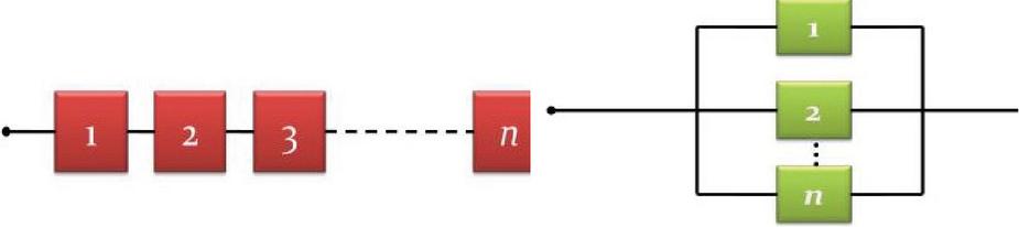
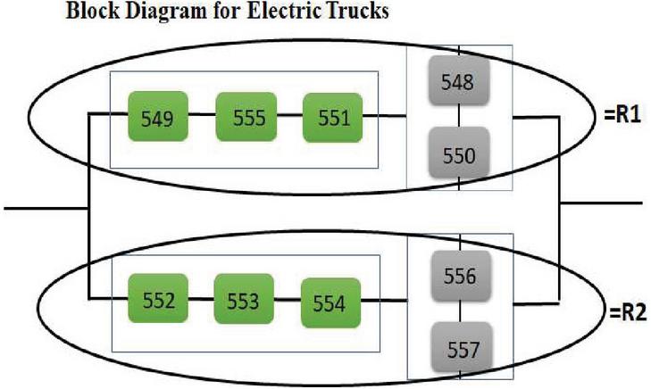
10 electric trucks are planned for 2 electric excavators in the field. In order to prevent the system from losing its functionality, 6 of the trucks (2x3) were connected in series, taking into account the requirement that 3 trucks for each excavator should be in operation. The other 4 trucks (2 $+$ 2) are connected in parallel.

The trucks that are planned to be connected in series are arranged as higher reliability trucks in order to ensure high reliability of the system, and trucks with low reliability are arranged as parallel connection.

Accordingly, serially connected truck door numbers are 549, 551, 555, 552, 553 and 554, respectively. Parallel trucks are the ones with door number 548, 550, 556, 557. System block diagram is as below. System reliability of the electric trucks used in the Manisa-Soma coal field was calculated according to the serial-parallel system.

According to this;

$R1(1000min.)$	$=R549xR555xR551x$
	$\mathrm{\hspace{1em}}\times [1-((1-R548)x(1-R550))$
	$=(61,26\%*77,04\%*56,42\%)$
	$\mathrm{\hspace{1em}}*[1-(1-41,53\%)*(1-36,89\%)]$
	$=16,80\%$
$R2(1000min)$	$=R552xR553xR554x$
	$\mathrm{\hspace{1em}}\times (1-((1-R556)x(1-R557))$
	$=(51,10\%*57,37\%*49,28\%)$
	$\mathrm{\hspace{1em}}*[1-(1-26,31\%)*(1-48,34\%)]$
	$=8,94\%$
$\mathit{R}\mathit{s}\mathit{y}\mathit{s}\mathit{t}\mathit{e}\mathit{m}(\mathbf{1000}\mathit{m}\mathit{i}\mathit{n})$	$=\mathbf{1}-(\mathbf{1}-\mathit{R}\mathbf{1})\mathit{x}(\mathbf{1}-\mathit{R}\mathbf{2})$
	$=[\mathbf{1}-(\mathbf{1}-\mathbf{16},\mathbf{80}\mathbf{\%})\mathbf{*}(\mathbf{1}-\mathbf{8},\mathbf{94}\mathbf{\%})$
	$=\mathbf{24},\mathbf{24}\mathbf{\%}$
$R1(500min)$	$=(77,20\%*84,46\%*74,02\%)$
	$\mathrm{\hspace{1em}}*[1-(1-56,94\%)*(1-55,90\%)]$
	$=39,09\%$
$R2(500min.)$	$=(70,01\%*85,64\%*68,15\%)$
	$\mathrm{\hspace{1em}}*[1-(1-40,02\%)*(1-69,07\%)]$
	$=33,28\%$
$\mathit{R}\mathit{s}\mathit{y}\mathit{s}\mathit{t}\mathit{e}\mathit{m}(\mathbf{500}\mathit{m}\mathit{i}\mathit{n})$	$=\mathbf{1}-(\mathbf{1}-\mathit{R}\mathbf{1})\mathit{x}(\mathbf{1}-\mathit{R}\mathbf{2})$
	$=[\mathbf{1}-(\mathbf{1}-\mathbf{39},\mathbf{09}\mathbf{\%})\mathbf{*}(\mathbf{1}-\mathbf{33},\mathbf{28}\mathbf{\%})$
	$=\mathbf{59},\mathbf{36}\mathbf{\%}$
$R1(250min.)$	$=(87,22\%*87,49\%*85,38\%)$
	$\mathrm{\hspace{1em}}*[1-(1-69,17\%)*(1-71,24\%)]$
	$=59,37\%$
$R2(250min.)$	$=(82,75\%*95,77\%*81,24\%)$
	$\mathrm{\hspace{1em}}*[1-(1-53,36\%)*(1-82,83\%)]$
	$=59,22\%$
$\mathit{R}\mathit{s}\mathit{y}\mathit{s}\mathit{t}\mathit{e}\mathit{m}(\mathbf{250}\mathit{m}\mathit{i}\mathit{n})$	$=\mathbf{1}-(\mathbf{1}-\mathit{R}\mathbf{1})\mathit{x}(\mathbf{1}-\mathit{R}\mathbf{2})$
	$=[\mathbf{1}-(\mathbf{1}-\mathbf{59},\mathbf{73}\mathbf{\%})\mathbf{*}(\mathbf{1}-\mathbf{59},\mathbf{22}\mathbf{\%})$
	$=\mathbf{83},\mathbf{43}\mathbf{\%}$

The reliability of the combined system is 24% for 1000 minutes (approximately 16 hours), while the reliability is 83% for a period of approximately 4 hours. In other words, the probability of trucks failure within 1000 minutes is 76%.

Repair times should be minimized in order to keep the trucks working more actively, and it will be appropriate to establish a preventive repair understanding and perform predictive maintenance studies by analyzing all trucks according to the types of malfunctions.

4 Result

✓ With 125 failures, the truck numbered 550 with the most breakdowns is followed by the truck numbered 552 with 121 breakdowns. Trucks with the least breakdowns are 555 with 67 failures and 551 with 68 failures, respectively.

✓ The longest repair period belongs to truck number 548 with 387 hours, and truck number 556 is the truck with the longest repair time with 336 hours. Trucks with the least repair time are 554 with 134 hours and truck number 549 with 145 hours.

✓ Trucks with the highest average mean time between failure (MTBF) are the trucks numbered 549 with 2355 minutes 555 and 2253 minutes, respectively. The lowest mean time to failure (MTTF) is 553 with 95 minutes and 551 with 129 minutes.

✓ While the data related to the working times between failures are mostly weibull distribution, repair time data are lognormal distribution.

✓ According to the analysis results, the trucks with the highest reliability are 555 with 77% and 549 with 61%. The least reliable trucks are 556 with 26%, 550 with 36% and 548 with 41%.

✓ Trucks with the highest maintainability rates are 553 with 73%, 551 with 62% and 554 with 56%, while the trucks with the lowest maintenance ease are 42% to 549, 44% to 556 and 45% to 548.

✓ The possibility of repairing the electric truck with door number 553 within 2 hours is 80%. The 551 truck will take 5.5 hours to be repaired with a 95% probability, while the 551 truck will have been repaired with a 95% probability of 10,167 hours and the truck number 554 in 8,25 hours. Other trucks can be repaired with 95% reliability in over 12 hours.

✓ When the availability rates are examined, the trucks numbered 553 with 92%, 549 with 91% and 554 with 90% have the highest availability rates. Trucks with the lowest availability rate are 556 with 73% and 548 with 83%.

✓ 10 electric trucks in the establisment are arranged for 2 electric excavators, 5 of them each, and it has a series-parallel combined system. As a result of system reliability calculations; The 16-hour reliability rate was calculated as 24%, the 8-hour reliability rate was 59%, and the 4-hour reliability rate was 83%.

✓ As a result of all these analyzes, it is necessary to increase the reliability level of the trucks and the system by starting the preventive repair-maintenance and predictive repair maintenance works as soon as possible in order to keep the trucks used in the operation in more.

References

[1] Jolly, S. S. and Wadhwa, S S. (2004). Reliability, availability and mainainability study of high precision special purpose manufacturing machines. Journal of Scientific & Industrial Research. 63, 512–517.

[2] Elevli, S. (1996). Preparing a computer-aided repair-maintenance program to increase the efficiency and productivity of equipment in mining operations. Master Thesis, Cumhuriyet Üniversity, Sivas, Turkey.

[3] Bentley, J.P. 1993. An introduction to Reliability and Quality Engineering. Logman Scientific and Technical. John Wiley & Sons, Inc. New York.

[4] Andrews, J.D., Moss, T.R. 2002. Reliability and Risk Assessment. Second Edition. Professional Engineering Publishing Limited: London and Bury St Edmunds, UK. 540s.

[5] Moss, T.R. 2005. The Reliability Data Handbook. Professional Engineering Publishing Limited: London and Bury St Edmunds, UK. 287s.

[6] Hahn, G.J., Shapiro, S.S. 1967. Statistical Models in Engineering. John Wiley & Sons, Inc.

[7] Meeker, W. Q., Escobar, L. A. 1998. Statistical Methods for Reliability Data. John Wiley & Sons Inc.

[8] Şentürk, A. (1998) Life Data Analysis and An Application, Phd Thesis, Uludağ Üniversity, Bursa, Turkey.

[9] Ebelign, C. E. (1997) Reliability and Maintainability Engineering, McGraw-Hill International Editions.

[10] Uzgören, N., Elevli, S., Elevli, B. and Uysal, Ö. (2010). Reliability analysis of draglines’ mechanical failures. Maintenance and Reliability, 4.

[11] Lienig J., Bruemmer H. (2017). Reliability Analysis. Fundamentals of Electronic Systems Design. Springer International Publishing. pp. 45–73.

[12] Birolini A. (2013). Reliability Engineering: Theory and Practice, Springer, Berlin.

Biography

Sedat Toraman received the bachelor’s degree in mining engineering from İstanbul Technical University in 1992, the master’s degree in mining engineering from Çukurova University in 1995, and the doctorate degree in mining engineering from Çukurova University in 2016, respectively. He is currently working as an mining engineer at Turkey Directorate General of Coal Enterprises. His research areas include ram analysis, artificial neural networks, optimization.

Journal of Reliability and Statistical Studies, Vol. 16, Issue 1 (2023), 81–98.
doi: 10.13052/jrss0974-8024.1614
© 2023 River Publishers

Abstract

1 Introduction

2 Analysis of Electric Trucks Used in Manisa-Soma Open Pit Mining

3 System Reliability

4 Result

References

Biography