An Analysis of the Mean Chart Under OC Function for Correlated Data

Manzoor A. Khanday^*, Shiv Shankar Pandey, Akansha Rawat and Chukka Sowjanya

School of Chemical Engineering and Physical Science, Lovely Professional University, Punjab, India
E-mail: manzoorstat@gmail.com; pandeyshivshankar03@gmail.com; sowjanya.jhasmin@gmail.com
*Corresponding Author

Received 23 March 2023; Accepted 11 November 2023; Publication 12 February 2024

Abstract

In this paper, we determine and illustrate the effects of correlation between the observations on the operating characteristics curve, Type-I error and Average Run length. In addition, for different correlated coefficient the control limits have been developed. To study the effect of correlated observations the OC curves, Type-I error, ARL and factor A have been worked out using various equation and values are given in Tables 1 to 4. To give a visual comparison of OC function and ARL, curves have been drawn in Figures 1 to 6. It is found that correlation between observations seriously affected the OC, Type-I error, ARL and factor A for the mean chart when standards are known. When the center line and control limits are based on the large value. Thus, it will be healthy contribution in manufacturing process which tracks important product characteristics in industry.

Keywords: Correlation, X-bar chart, operating characteristic (OC) curve, average run length (ARL).

1 Introduction

In the manufacturing area, control charts are used to examine historical data, provide the basis for process capability studies, and serve as tools for monitoring the characteristics of processes to detect deviations from target values and from the statistical control. In research and engineering, control charts provide a method for tracking the stability of the measurement process and a way of examining the homogeneity of sets of data. It is a useful tool for data analysis and provides an easily understood way of displaying results. In forecasting, a control chart approach to examining errors can provide not only information concerning correction but also insight into improved modal formulation. The control limits of Shewhart control charts are exact only if the process characteristic under consideration is normally distributed. Not all the process are normally distributed, see Shewhart (1939), Fearell (1953).

The effect of correlation on the economic design of warning limit of X-bar charts is studied by Lin et al. (2003). The effect of double exponentially weighted moving average (DEWMA) model under Economic Design (ED) of $\overline{\mathrm{X}}$ control chart was studied by Manzoor A. Khanday and J. R. Singh (2020). The application of control charts to monitor time related measures in operational systems raise fundamental satisfied problems. The need for approaches that are robust with respect to data correlation and lack of normality are shown to be an essential requirement. In both manufacturing and service operations. Singh et al. (2013) studied the effect of correlated data on sampling plans. Industrial processes are often serially correlated. Serious errors concerning the state of statistical process control may result if the correlation structure of the observations is not considered. Malfunction of plant equipment, installation and degradation in process operation increases the operating cost of any chemical process industries. Thus, modern chemical industries need to operate as fault face as possible because faults that are present in a process increase the operating cost due to the increase in waste generation and products with undesired specification. Effective monitoring strategy not only from a safety and cost viewpoint, but also for the maintenance of yield and the product quality in a process as well. Che Din et al. (2011) analyzed and determined the technique used to determine the correlation coefficients between the process variables and quality variable while control chart with the calculated correlation coefficients is used to facilitate the fault detection and diagnosis algorithm.

2 Description of the Mean for Correlated Data

Let us suppose that the observations x${}_1$, x${}_2$, x${}_3$, …, x${}_{\mathrm{n}}$ follows a multivariate normal distribution with $E(x_i)=\mu$ (mean) and $V(x_i)={\sigma }^2$

$E(\overline{x})$	$=E\left({\displaystyle \frac{1}{n}}{\displaystyle \sum _{i=1}^n}{x}_i\right)={\displaystyle \frac{1}{n}}{\displaystyle \sum _{i=1}^n}E(x_i)={\displaystyle \frac{1}{n}}{\displaystyle \sum _{i=1}^n}\mu \mathit{\hspace{1em}}\because E(x_i)=\mu$
	$={\displaystyle \frac{1}{n}}(n\mu )=\mu$	(1)

And

$V(\overline{x})$	$=E({\overline{x}}^2)-{[E(\overline{x})]}^2=\left[E{\left({\displaystyle \frac{1}{n}}{\displaystyle \sum x_i}\right)}^2\right]-{\mu }^2$
$V(\overline{x})$	$={\displaystyle \frac{1}{n^2}}\mathrm{E}\left[{\displaystyle \sum ({\mathrm{x}}_i^2)}+{\displaystyle \sum _{i\ne }}{\displaystyle \sum _j}{x}_i{x}_j\right]-{\mu }^2$
$V(\overline{\mathrm{x}})$	$={\displaystyle \frac{1}{{\mathrm{n}}^2}}\left[\mathrm{E}\left({\displaystyle \sum {\mathrm{x}}_{\mathrm{i}}^2}\right)+\mathrm{E}\left({\displaystyle \sum _{i\ne }}{\displaystyle \sum _j}{\mathrm{x}}_{\mathrm{i}}{\mathrm{x}}_{\mathrm{j}}\right)\right]-{\mu }^2$	(2)

Since,

${\sigma }^2$	$={\displaystyle \frac{1}{\mathrm{n}}}{\displaystyle \sum {({\mathrm{x}}_{\mathrm{i}}-\mu )}^2}$
	$={\displaystyle \frac{1}{n}}{\displaystyle \sum \left[x_i^2+{\mu }^2-2\mu \sum x_i\right]}$
	$={\displaystyle \frac{1}{\mathrm{n}}}\left[{\displaystyle \sum {\mathrm{x}}_{\mathrm{i}}^2}+n{\mu }^2-2\mu {\displaystyle \sum x_{\mathrm{i}}}\right]$	(3)

Taking expectation on both sides to Equation (3), we get

${\sigma }^2$	$={\displaystyle \frac{1}{n}}\left[E\left({\displaystyle \sum x_i^2}\right)+n{\mu }^2-2\mu E\left({\displaystyle \sum x_i}\right)\right]$
${\sigma }^2$	$={\displaystyle \frac{1}{n}}\left[E\left({\displaystyle \sum x_i^2}\right)+n{\mu }^2-2\mu (n\mu )\right]$
${\sigma }^2$	$={\displaystyle \frac{1}{n}}\left[E\left({\displaystyle \sum {\mathrm{x}}_{\mathrm{i}}^2}-\mathrm{n}{\mu }^2\right)\right]$
$n{\sigma }^2$	$=E\left({\displaystyle \sum x_i^2}\right)-n{\mu }^2$
$\mathrm{or},E\left({\displaystyle \sum x_i^2}\right)$	$=n{\sigma }^2+n{\mu }^2=n({\sigma }^2+{\mu }^2)$

Also,

$$\rho =\frac{\mathrm{Cov}(x,y)}{{\sigma }_{\mathrm{x}}{\sigma }_{\mathrm{y}}}=\frac{\frac{1}{\mathrm{n}(n-1)}\left\{{\sum }_{i\ne }{\sum }_j{\mathrm{x}}_{\mathrm{i}}{\mathrm{x}}_{\mathrm{j}}\right\}-\overline{\mathrm{x}}\overline{\mathrm{y}}}{{\sigma }_x{\sigma }_y}$$

Here, $\overline{\mathrm{x}}=\overline{\mathrm{y}}=\mu$ and ${\sigma }_x={\sigma }_y=\sigma$, we get

$\rho ={\displaystyle \frac{\frac{1}{n(n-1)}\left\{{\sum }_{i\ne }{\sum }_{\mathrm{j}}{\mathrm{x}}_{\mathrm{i}}{\mathrm{x}}_{\mathrm{j}}\right\}-{\mu }^2}{{\sigma }^2}}$

${\sigma }^2\rho ={\displaystyle \frac{1}{n(n-1)}}\left\{{\displaystyle \sum _{i\ne }}{\displaystyle \sum _j}{\mathrm{x}}_{\mathrm{i}}{\mathrm{x}}_{\mathrm{j}}\right\}-{\mu }^2$

$n(n-1)\{{\sigma }^2\rho +{\mu }^2\}={\displaystyle \sum _{i\ne }}{\displaystyle \sum _j}{x}_i{x}_j$

Therefore,

$E\left({\displaystyle \sum _{i\ne }}{\displaystyle \sum _j}{\mathrm{x}}_{\mathrm{i}}{\mathrm{x}}_j\right)=n(n-1)\{\rho {\sigma }^2+{\mu }^2\}$

(4)

Therefore, Equation (2) becomes.

$V(\overline{x})$	$={\displaystyle \frac{1}{n^2}}[n({\sigma }^2+{\mu }^2)+n(n-1)\{\rho {\sigma }^2+{\mu }^2\}]-{\mu }^2$
$V(\overline{x})$	$={\displaystyle \frac{{\sigma }^2}{n}}+{\displaystyle \frac{{\mu }^2}{n}}+{\displaystyle \frac{(n-1)\rho {\sigma }^2}{n}}+{\displaystyle \frac{(n-1){\mu }^2}{n}}-{\mu }^2$
$V(\overline{x})$	$={\displaystyle \frac{{\sigma }^2}{n}}+{\displaystyle \frac{(n-1)\rho {\sigma }^2}{n}}+{\displaystyle \frac{(n-1){\mu }^2}{n}}+{\displaystyle \frac{{\mu }^2}{n}}-{\mu }^2$
$V(\overline{x})$	$={\displaystyle \frac{{\sigma }^2}{n}}[1+(n-1)\rho ]+{\mu }^2\left({\displaystyle \frac{n-1}{n}}+{\displaystyle \frac{1}{n}}-1\right)$
$V(\overline{x})$	$={\displaystyle \frac{{\sigma }^2}{n}}[1+(n-1)\rho ]+{\mu }^2\left({\displaystyle \frac{n-1+1-n}{n}}\right)$
$V(\overline{x})$	$={\displaystyle \frac{{\sigma }^2}{n}}[1+(n-1)\rho ]$	(5)
$V(\overline{x})$	$={\displaystyle \frac{{\sigma }^2}{n}}{T}^2$
$where,T^2$	$=[1+(n-1)\rho ]$

The ability of mean charts to detect shifts in process quality is described by their OC curves. The control chart for mean is set up by drawing the central line at the process average $\mu$ and control limits at $\mu \pm \frac{k\sigma }{\sqrt{n}}$, where n is the sample size. The OC function gives the probability that the control chart indicates the value $\mu$, as the process average, when it is actually not $\mu$ but ${\mu }^{\prime }=(\mu +\frac{\gamma \sigma T}{\sqrt{n}})$. It is derived by integrating the distribution of mean with ${\mu }^{\prime }$ as the process average, between the limits of the control chart.

The observed density function with mean $\mu$ and standard deviation $\sigma$ will be written as,

$$f(x)=\frac{1}{\sigma }\varphi \left(\frac{x-\mu }{\sigma }\right)$$

(6)

The distribution of observed sample mean is given by.

$$f(\overline{x})=\frac{\sqrt{n}}{\sigma T}\left\{\varphi \frac{(x-\mu )\sqrt{n}}{\sigma T}\right\}$$

(7)

The OC function is obtained after replacing $\mu$ in Equation (7) by ${\mu }^{\prime }$ and integrating it between the limits of the control charts as

$L(P)$	$={\displaystyle {\int }_{\mu -\frac{k\sigma }{\sqrt{n}}}^{\mu +\frac{k\sigma }{\sqrt{n}}}}f(\overline{x})\mathit{d}\overline{x}$	(8)
$L(P)$	$={\displaystyle \frac{\sqrt{n}}{\sigma T}}{\displaystyle {\int }_{\mu -\frac{k\sigma }{\sqrt{n}}}^{\mu +\frac{k\sigma }{\sqrt{n}}}}\varphi \left[{\displaystyle \frac{(\overline{x}-{\mu }^{\prime })\sqrt{n}}{\sigma T}}\right]\mathit{d}\overline{x}$
	$={\displaystyle \frac{\sqrt{n}}{\sigma T}}{\displaystyle {\int }_{\mu -\frac{k\sigma }{\sqrt{n}}}^{\mu +\frac{k\sigma }{\sqrt{n}}}}\varphi \left[{\displaystyle \frac{\left(\overline{x}-\mu -\frac{\gamma \sigma T}{\sqrt{n}}\right)\sqrt{n}}{\sigma T}}\right]\mathit{d}\overline{x}$
	$={\displaystyle \frac{\sqrt{n}}{\sigma T}}{\displaystyle {\int }_{\mu -\frac{k\sigma }{\sqrt{n}}}^{\mu +\frac{k\sigma }{\sqrt{n}}}}\varphi \left[{\displaystyle \frac{(\overline{x}-\mu )\sqrt{n}}{\sigma T}}-{\displaystyle \frac{\gamma \sigma T}{\sigma T}}\right]\mathit{d}\overline{x}$
	$={\displaystyle \frac{\sqrt{n}}{\sigma T}}{\displaystyle {\int }_{\mu -\frac{k\sigma }{\sqrt{n}}}^{\mu +\frac{k\sigma }{\sqrt{n}}}}\varphi \left[{\displaystyle \frac{(\overline{x}-\mu )\sqrt{n}}{\sigma T}}-\gamma \right]\mathit{d}\overline{x}$	(9)

putting,

${\displaystyle \frac{\overline{x}-\mu }{\sigma T/\sqrt{n}}}=y\Rightarrow d\overline{x}={\displaystyle \frac{\sigma T}{\sqrt{n}}}dy$

Therefore, the limits of $y=\pm \frac{k}{T}$

$L(P)={\displaystyle \frac{\sqrt{n}}{\sigma T}}{\displaystyle \frac{\sigma T}{\sqrt{n}}}{\displaystyle {\int }_{-\frac{k}{T}}^{+\frac{k}{T}}}\varphi (y-\gamma )\mathit{d}y$

(10)

Now again putting $y-\gamma =t\Rightarrow dy=dt$

$L(P)$	$={\displaystyle {\int }_{-(\frac{k}{T}+\gamma )}^{\frac{k}{T}-\gamma }}\varphi (t)\mathit{d}y$	(11)
$L(P)$	$={\displaystyle {\int }_{-\propto }^{+\propto }}\varphi (t)\mathit{d}t-{\displaystyle {\int }_{-\propto }^{-(\frac{k}{T}+\gamma )}}\varphi (t)\mathit{d}t-{\displaystyle {\int }_{\frac{k}{T}-\gamma }^{\propto }}\varphi (t)\mathit{d}t$
	$=1-\left(1-{\displaystyle {\int }_{-\propto }^{(\frac{k}{T}+\gamma )}}\varphi (t)\mathit{d}t\right)-{\displaystyle {\int }_{\frac{k}{T}-\gamma }^{\propto }}\varphi (t)\mathit{d}t$
	$={\displaystyle {\int }_{-\propto }^{(\frac{k}{T}+\gamma )}}\varphi (t)\mathit{d}t-{\displaystyle {\int }_{\frac{k}{T}-\gamma }^{\propto }}\varphi (t)\mathit{d}t$
	$=\mathrm{\Phi }\left({\displaystyle \frac{k}{T}}+\gamma \right)+{\displaystyle {\int }_{\propto }^{(\frac{k}{T}-\gamma )}}\varphi (t)\mathit{d}t.$	(12)

Transforming variable t in z by putting $t=-z$, we have

$L(P)=\mathrm{\Phi }\left({\displaystyle \frac{k}{T}}+\gamma \right)-{\displaystyle {\int }_{-\propto }^{-(\frac{k}{T}-\gamma )}}\varphi (-z)\mathit{d}z.$

we know that $\varphi (-z)=\varphi (z)$.

Therefore,

$L(P)$	$=\mathrm{\Phi }\left({\displaystyle \frac{k}{T}}+\gamma \right)-{\displaystyle {\int }_{-\propto }^{-(\frac{k}{T}-\gamma )}}\varphi (z)\mathit{d}z.$
$L(P)$	$=\mathrm{\Phi }\left({\displaystyle \frac{k}{T}}+\gamma \right)-\left[1-\mathrm{\Phi }\left({\displaystyle \frac{k}{T}}-\gamma \right)\right]$
$L(P)$	$=\mathrm{\Phi }\left({\displaystyle \frac{k}{T}}+\gamma \right)+\mathrm{\Phi }\left({\displaystyle \frac{k}{T}}-\gamma \right)-1$	(13)

The error of first kind gives the probability of searching for assignable causes when in fact there are no such causes or in other words, it is the probability that the sample values lie outside the control limits when the process average and variation remain unchanged, and it is given by.

$\alpha$	$=1-{\displaystyle {\int }_{\mu -k\sigma /\sqrt{n}}^{\mu +k\sigma /\sqrt{n}}}f(\overline{x})\mathit{d}\overline{x}$
	$=2\mathrm{\Phi }(-k/T)$	(14)

The (ARL) for the mean chart for correlated data can be expressed as,

$\mathit{ARL}$	$={\displaystyle \frac{1}{p(\mathit{one}\mathit{point}\mathit{plots}\mathit{out}\mathit{of}\mathit{control})}}$
$\mathit{ARL}$	$={\displaystyle \frac{1}{\alpha }}$	(15)

The three sigma limits for correlated data are $\overline{x}\pm \frac{3\sigma T}{\sqrt{n}}$

$$i.e.,\overline{x}\pm A\sigma .$$

Where,

$$A=\frac{3T}{\sqrt{n}}$$

(16)

Table 1 Values of OC function for correlated data

		$k=2$					$k=3$
		$P$					$\rho$
n	$\gamma$	0	0.2	0.5	0.6	0.8	1	0	0.2	0.5	0.6	0.8	1
	0	0.9545	0.8640	0.7518	0.7219	0.6709	0.6289	0.9973	0.9747	0.9167	0.8963	0.8568	0.8203
	$\pm$0.5	0.9270	0.8158	0.6947	0.6641	0.6129	0.5718	0.9936	0.9556	0.8782	0.8534	0.8077	0.7672
	$\pm$1	0.8400	0.6818	0.5459	0.5152	0.4663	0.4289	0.9772	0.8912	0.7648	0.7304	0.6717	0.6241
	$\pm$1.5	0.6912	0.4949	0.3610	0.3341	0.2935	0.2641	0.9332	0.7691	0.5911	0.5496	0.4841	0.4348
	$\pm$2	0.5000	0.3050	0.1982	0.1790	0.1514	0.1326	0.8413	0.5933	0.3943	0.3544	0.2957	0.2547
5	$\pm$2.5	0.3085	0.1564	0.0891	0.0783	0.0635	0.0538	0.6915	0.3959	0.2212	0.1913	0.1500	0.1233
	$\pm$3	0.1587	0.0656	0.0325	0.0277	0.0214	0.0176	0.5000	0.2225	0.1024	0.0849	0.0622	0.0486
	$\pm$3.5	0.0668	0.0223	0.0095	0.0079	0.0058	0.0046	0.3085	0.1031	0.0385	0.0305	0.0209	0.0154
	$\pm$4	0.0228	0.0060	0.0022	0.0018	0.0012	0.0009	0.1587	0.0389	0.0117	0.0088	0.0056	0.0039
	$\pm$4.5	0.0062	0.0013	0.0004	0.0003	0.0002	0.0002	0.0668	0.0118	0.0028	0.0020	0.0012	0.0008
	$\pm$5	0.0013	0.0002	0.0001	0.0000	0.0000	0.0000	0.0228	0.0029	0.0005	0.0004	0.0002	0.0001
	0	0.9545	0.8327	0.6062	0.5708	0.5151	0.4729	0.9973	0.9270	0.7992	0.7643	0.7052	0.6572
	$\pm$0.5	0.9270	0.7115	0.5498	0.5159	0.4633	0.4240	0.9936	0.8910	0.7445	0.7077	0.6472	0.5995
	$\pm$1	0.8400	0.5633	0.4095	0.3804	0.3368	0.3053	0.9772	0.7835	0.5986	0.5593	0.4987	0.4539
	$\pm$1.5	0.6912	0.3768	0.2494	0.2280	0.1974	0.1763	0.9332	0.6147	0.4099	0.3731	0.3201	0.2835
	$\pm$2	0.5000	0.2098	0.1235	0.1106	0.0930	0.0815	0.8413	0.4179	0.2350	0.2071	0.1693	0.1450
10	$\pm$2.5	0.3085	0.0959	0.0494	0.0432	0.0351	0.0300	0.6915	0.2397	0.1110	0.0943	0.0730	0.0601
	$\pm$3	0.1587	0.0355	0.0158	0.0135	0.0106	0.0088	0.5000	0.1137	0.0426	0.0348	0.0254	0.0201
	$\pm$3.5	0.0668	0.0106	0.0041	0.0034	0.0025	0.0021	0.3085	0.0439	0.0132	0.0103	0.0071	0.0054
	$\pm$4	0.0228	0.0025	0.0008	0.0007	0.0005	0.0004	0.1587	0.0137	0.0033	0.0024	0.0016	0.0011
	$\pm$4.5	0.0062	0.0005	0.0001	0.0001	0.0001	0.0001	0.0668	0.0034	0.0006	0.0005	0.0003	0.0002
	$\pm$5	0.0013	0.0001	0.0000	0.0000	0.0000	0.0000	0.0228	0.0007	0.0001	0.0001	0.0000	0.0000
	0	0.9545	0.6951	0.5205	0.4858	0.4331	0.3944	0.9973	0.8762	0.7112	0.6722	0.6096	0.5614
	$\pm$0.5	0.9270	0.6370	0.4683	0.4359	0.3872	0.3518	0.9936	0.8299	0.6532	0.6142	0.5531	0.5070
	$\pm$1	0.8400	0.4890	0.3409	0.3148	0.2766	0.2496	0.8400	0.4890	0.3409	0.3148	0.2766	0.2496
	$\pm$1.5	0.6912	0.3120	0.2003	0.1826	0.1578	0.1408	0.9332	0.5144	0.3250	0.2944	0.2516	0.2226
	$\pm$2	0.5000	0.1638	0.0946	0.0849	0.0717	0.0630	0.8413	0.3222	0.1727	0.1521	0.1248	0.1074
15	$\pm$2.5	0.3085	0.0700	0.0358	0.0315	0.0259	0.0224	0.6915	0.1682	0.0748	0.0638	0.0500	0.0417
	$\pm$3	0.1587	0.0242	0.0108	0.0093	0.0074	0.0063	0.5000	0.0720	0.0262	0.0216	0.0161	0.0129
	$\pm$3.5	0.0668	0.0067	0.0026	0.0022	0.0017	0.0014	0.3085	0.0249	0.0074	0.0058	0.0041	0.0032
	$\pm$4	0.0228	0.0015	0.0005	0.0004	0.0003	0.0002	0.1587	0.0069	0.0016	0.0013	0.0008	0.0006
	$\pm$4.5	0.0062	0.0003	0.0001	0.0001	0.0000	0.0000	0.0668	0.0015	0.0003	0.0002	0.0001	0.0001
	$\pm$5	0.0013	0.0000	0.0000	0.0000	0.0000	0.0000	0.0228	0.0003	0.0000	0.0000	0.0000	0.0000

Table 2 Values of Alpha for different n and k under correlated data

		$\rho$
n	k	0	0.2	0.5	0.6	0.8	1
	0.0	1.0000	1.0000	1.0000	1.0000	1.0000	1.0000
	0.5	0.6171	0.7094	0.7728	0.7863	0.8073	0.8231
	1.0	0.3173	0.4561	0.5637	0.5876	0.6256	0.6547
5	1.5	0.1336	0.2636	0.3865	0.4159	0.4642	0.5023
	2.0	0.0455	0.1360	0.2482	0.2781	0.3291	0.3711
	2.5	0.0124	0.0624	0.1489	0.1752	0.2225	0.2636
	3.0	0.0027	0.0253	0.0833	0.1037	0.1432	0.1797
	0.0	1.0000	1.0000	1.0000	1.0000	1.0000	1.0000
	0.5	0.6171	0.7651	0.8312	0.8433	0.8614	0.8744
	1.0	0.3173	0.5501	0.6698	0.6926	0.7269	0.7518
10	1.5	0.1336	0.3700	0.5224	0.5532	0.6004	0.6353
	2.0	0.0455	0.2320	0.3938	0.4292	0.4849	0.5271
	2.5	0.0124	0.1352	0.2864	0.3230	0.3826	0.4292
	3.0	0.0027	0.0730	0.2008	0.2357	0.2948	0.3428
	0.0	1.0000	1.0000	1.0000	1.0000	1.0000	1.0000
	0.5	0.6171	0.7976	0.8597	0.8705	0.8862	0.8973
	1.0	0.3173	0.6080	0.7237	0.7443	0.7746	0.7963
15	1.5	0.1336	0.4416	0.5959	0.6247	0.6676	0.6985
	2.0	0.0455	0.3049	0.4795	0.5142	0.5669	0.6056
	2.5	0.0124	0.1997	0.3768	0.4148	0.4741	0.5186
	3.0	0.0027	0.1238	0.2888	0.3278	0.3904	0.4386

Table 3 Values of ARL for correlated data

		$\rho$
n	k	0	0.2	0.5	0.6	0.8	1
	0.0	1.0000	1.0000	1.0000	1.0000	1.0000	1.0000
	0.5	1.6205	1.4097	1.2939	1.2718	1.2388	1.2150
	1.0	3.1515	2.1927	1.7740	1.7019	1.5985	1.5274
5	1.5	7.4842	3.7943	2.5875	2.4042	2.1542	1.9907
	2.0	21.9779	7.3509	4.0288	3.5961	3.0385	2.6947
	2.5	80.5196	16.0237	6.7153	5.7091	4.4941	3.7943
	3.0	370.3983	39.4519	12.0099	9.6393	6.9815	5.5644
	0.0	1.0000	1.0000	1.0000	1.0000	1.0000	1.0000
	0.5	1.6205	1.3070	1.2031	1.1858	1.1609	1.1437
	1.0	3.1515	1.8179	1.4929	1.4438	1.3757	1.3301
10	1.5	7.4842	2.7025	1.9141	1.8076	1.6656	1.5742
	2.0	21.9779	4.3104	2.5396	2.3299	2.0622	1.8972
	2.5	80.5196	7.3983	3.4914	3.0955	2.6134	2.3299
	3.0	370.3983	13.6990	4.9795	4.2430	3.3921	2.9173
	0.0	1.0000	1.0000	1.0000	1.0000	1.0000	1.0000
	0.5	1.6205	1.2538	1.1632	1.1488	1.1284	1.1145
	1.0	3.1515	1.6448	1.3818	1.3435	1.2909	1.2559
15	1.5	7.4842	2.2645	1.6782	1.6009	1.4979	1.4316
	2.0	21.9779	3.2797	2.0855	1.9448	1.7639	1.6513
	2.5	80.5196	5.0081	2.6542	2.4106	2.1091	1.9282
	3.0	370.3983	8.0767	3.4621	3.0504	2.5615	2.2801

Table 4 Values of factor A for correlated data

	$n=5$
	$\rho$
n	0	0.2	0.5	0.6	0.8	1
2	2.1213	2.3238	2.5981	2.6833	2.8460	3.0000
3	1.7321	2.0494	2.4495	2.5690	2.7928	3.0000
4	1.5000	1.8974	2.3717	2.5100	2.7659	3.0000
5	1.3416	1.8000	2.3238	2.4739	2.7495	3.0000
6	1.2247	1.7321	2.2913	2.4495	2.7386	3.0000
7	1.1339	1.6818	2.2678	2.4319	2.7308	3.0000
8	1.0607	1.6432	2.2500	2.4187	2.7249	3.0000
9	1.0000	1.6125	2.2361	2.4083	2.7203	3.0000
10	0.9487	1.5875	2.2249	2.4000	2.7166	3.0000
11	0.9045	1.5667	2.2156	2.3932	2.7136	3.0000
12	0.8660	1.5492	2.2079	2.3875	2.7111	3.0000
13	0.8321	1.5342	2.2014	2.3826	2.7090	3.0000
14	0.8018	1.5213	2.1958	2.3785	2.7071	3.0000
15	0.7746	1.5100	2.1909	2.3749	2.7055	3.0000
16	0.7500	1.5000	2.1866	2.3717	2.7042	3.0000
17	0.7276	1.4912	2.1828	2.3689	2.7029	3.0000
18	0.7071	1.4832	2.1794	2.3664	2.7019	3.0000
19	0.6882	1.4761	2.1764	2.3642	2.7009	3.0000
20	0.6708	1.4697	2.1737	2.3622	2.7000	3.0000
21	0.6547	1.4639	2.1712	2.3604	2.6992	3.0000
22	0.6396	1.4585	2.1690	2.3587	2.6985	3.0000
23	0.6255	1.4536	2.1669	2.3572	2.6978	3.0000
24	0.6124	1.4491	2.1651	2.3558	2.6972	3.0000
25	0.6000	1.4450	2.1633	2.3546	2.6967	3.0000

3 Illustrations and Conclusions

To study the effect of correlated observations the OC, Type–I error, ARL, and factor A have been worked out using Equations (2), (2), (15) and (16) respectively. The values of OC for k $=$ 2, 3 and n $=$ 5, 10, 15 for different sizes of correlation coefficient $\rho$ $=$ 0, 0.2, 0.5, 0.8 and 1 are given in Table 1. From Table 1 it is evident that the values of OC are affected seriously as the correlation between the observations increases. From Table 1 the value of OC function for uncorrelated variable (r $=$ 0), k $=$ 2, n $=$ 5 and g $=$ 0 is 0.9545, while for r $=$ 0.2, 0.5, 0.6, 0.8, 1.0 the values are 0.8640, 0.7518, 0.7219, 0.6709, 0.6289 respectively. The values of OC for k $=$ 3 are 0.9923, 0.9747, 0.9167, 0.8963, 0.8568, 0.8203. It is occasionally useful to study the OC function for the chart used to analyze past data. From Table 1 It is seen that when the mean value is shifted from its target value viz. $\gamma =\pm 3$, $k=3,n=5$ for uncorrelated case i.e., $r=0$ and $r=0.2$, 0.5, 0.6, 0.8, and 1.0 the OC values are 0.5000, 0.2225, 0.1024, 0.0849, 0.0622, and 0.0486 respectively. This shows that OC functions are seriously affected when the mean shifts from its target values.

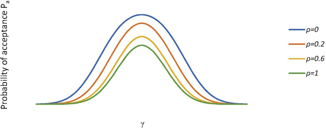
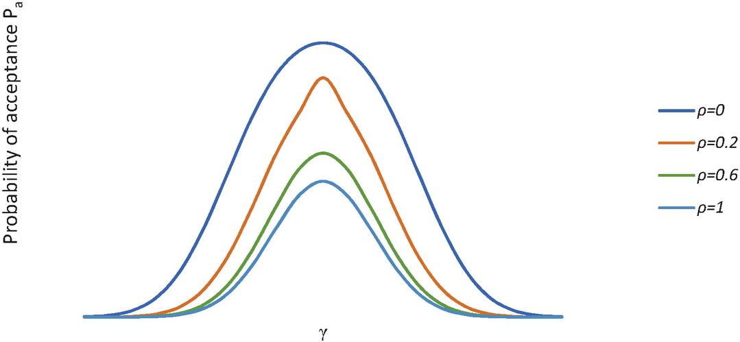
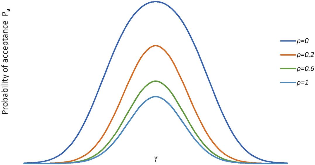
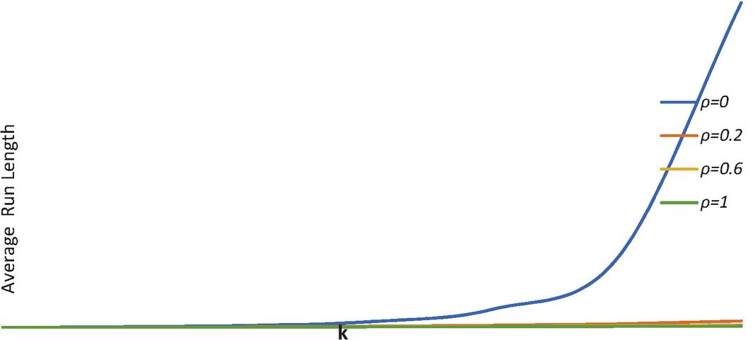
To give a visual comparison of OC functions, curves have been drawn in Figures 1 to 5 for $k=2$, 3 and $n=5$, 10, 15, It is seen from all the figures that correlation seriously affects the OC curve of the normal theory for the mean chart. Note that the OC curve increases very rapidly when we are moving towards the target mean and decreases when we are shifting away from the target values. From Figures 1 to 5 it is easily seen that correlation among the observations has a dramatic effect on the OC curves. It is seen that OC curve for $k=2$ is better than $k=3$, as seen from Figures 1 to 5 for $k=2$ the OC curve shows better protection to both producer and consumer. And it is also seen that by increasing (n) the probability of accepting correlated data decreases.

Figure 1 OC curve for $k=2$ and $n=5$.

Figure 2 OC curve for $k=2$ and $n=10$.

Figure 3 OC curve for $k=2$ and $n=15$.

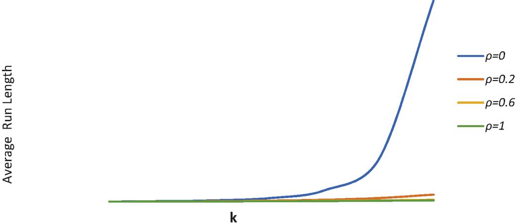
Figure 4 ARL curve for $n=5$.

Figure 5 ARL curve for $n=10$.

Figure 6 ARL curve for $n=15$.

For various correlation coefficients the values of a are given in the Table 2 for different values of k and n, the Table 2 clearly indicates that for $k=2$ to 3, $n=5$, 10, 15 the error of the first kind is seriously affected when the correlation is present in observations. The value increases as the correlation between the observations increases for all n. For uncorrelated observations the value of a is same for all n for corresponding k. But with increase in n the values of a increases for corresponding values of k and $r$.

The values of ARL are given in Table 3 in general, the expected number of samples taken before the shift is detected is just the average run length. Table 3 clearly indicates that ARL decreases as correlation coefficient increases. The effects are negligible for $k=0$ to 1.5, for $k=1.5$ the ARL is seriously affected as the correlation coefficient increases. From table it is seen that for uncorrelated observations ARL is same for all n, but there is decrease in ARL as n increases for corresponding value of k, and this change increases rapidly as correlation coefficient increases.

The values of factor A for $n=2$ to 25 and for different correlation coefficient are calculated and shown in Table 4. As Table 4 indicates, when n increases, Factor A decreases. Therefore, the control limits tend to become tighter and thereby more sensitive to detect changes in the process, where n is the number of subgroups used to calculate $\overline{x}$ chart for correlated observations. As correlation coefficient increases, factor A increases and thereby becomes less sensitive to detect changes in the process. When there is perfect correlation between observation the factor A is same for all n i.e.,3, the maximum control limit is independent of n. Thus Table 4 indicates that factor A is seriously affected with correlated observation.

The above discussion shows that correlation between observations in industry seriously affected the OC, type-I errors, ARL, and factor A for the mean chart when standards are known. When the center line and control limits are based on the large value. The process can very easily be judged in-control when, in fact, it is not.

References

[1] Lin, H. R., Chou, C. Y. and Chen, C. H. (2003): The effect of correlation on the economic design of warning limit X-bar charts; The International Journal of Advanced Manufacturing Technology, Vol. 22, pp. 3–4.

[2] Che Dinetal, N.S., Abdul Samad, N.A.F. and Chin, S.Y. (2011): Fault detection and diagnosis for Gas Density Monitoring using multivariate statistical process control. Journal of applied sciences, 11: 2400–2405.

[3] Singh J. R, Sankle R., and M. Ahmad Khanday (2013): Variables Sampling Plan for Correlated Data. Journal of Modern Applied Statistical Methods, Vol 12, Issue 2.

[4] Zameer Abbas, Hafiz Zafar Nazir, Noureen Akhtar. Muhammad Riaz, and Muhammad Abid (2020): On designing a progressive mean chart for efficient monitoring of process location. Quality and Reliability Engineering. April 2020, DOI: 10.1002/qre.2655.

[5] Shewhart, W.A. (1939): Statistical methods from the viewpoint of Quality Control, Republished in 1986 by Dover Publications New York: 12, 54.

[6] Fearell, E. B. (1953): Control Charts using Median & Mid Ranges, Industrial Quality Control, 9:30–32.

[7] Che Dinetal, N.S., Abdul Samad, N.A.F. and Chin, S.Y. (2011): Fault detection and diagnosis for Gas Density Monitoring using multivariate statistical process control. Journal of applied sciences, 11: 2400–2405.

[8] Manzoor A. Khanday and J. R. Singh (2020): Economic Design of X̄ Control Chart under Double EWMA. Journal of Modern Applied Statistical Methods.

Biographies

Manzoor A. Khanday was born on April 24, 1979, in a mountainous region in Anantnag Kashmir. He received preliminary education from HSS Srigufwara. He completed Bachelors from G.D.C Boys Anantnag, and pursued masters from the University of Kashmir, Srinagar. Following this, Dr. Manzoor Ahmad completed his Doctor of Philosophy from the Department of Statistics, Vikram University Ujjain, India. His research interests primarily include Economic Design of control charts, Statistical Quality Control, and has published more than twelve research papers in national and international journals. Presently Dr. Manzoor Ahmad is an Assistant Professor at Lovely Professional University Punjab India.

Shiv Shankar Pandey is a second-year M. Sc. Statistics and Data Science student at the Lovely Professional University Punjab India. He received bachelor’s degree in Mathematics from Calcutta University India. He is interested in Data Analytics and Machine Learning.

Akansha Rawat, is a third-year B. Sc. Hon. Mathematics student at the Lovely Professional University Punjab India. she passed 10$+$2, from Haryana India. She is interested in Data Analytics, Business Administration.

Chukka Sowjanya is a second-year M. Sc. Statistics and Data Science student at the Lovely Professional University Punjab India. she received a bachelor’s degree in Statistics from Andhra University India. She is interested in Data Analytics, Research areas like sampling, probability.

Journal of Reliability and Statistical Studies, Vol. 16, Issue 2 (2023), 281–296.
doi: 10.13052/jrss0974-8024.1625
© 2024 River Publishers

Abstract

1 Introduction

2 Description of the Mean for Correlated Data

3 Illustrations and Conclusions

References

Biographies