Accelerated Failure Time Models with Applications to Endometrial Cancer Survival Data

Manas Ranjan Tripathy¹, Prafulla Kumar Swain^2,*, Pravat Kumar Sarangi¹ and S. S. Pattnaik³

¹Department of Statistics, Ravenshaw University, Cuttack, Odisha, India
²Department of Statistics, Utkal University, Bhubaneswar, Odisha, India
³Department of Gynae Oncology, AHPGIC, Cuttack, Odisha, India
E-mail: prafulla86@gmail.com
^∗Corresponding Author

Received 31 October 2021; Accepted 21 January 2022; Publication 31 March 2023

Abstract

The objective of this study is to determine the significant predictors of endometrial cancer using accelerated failure time models (AFTM). We have demonstrated the applications of AFTM viz. Exponential, Weibull, Log-normal, Log-logistic, Gompertz, Gamma and Generalized Gamma AFTM, as an alternative of Cox proportional hazard model. Data for the analysis was collected from Acharya Harihar Post Graduate Institute of Cancer (AHPGIC), Cuttack, Odisha during the period 2016–20. Based on the lowest Akaike Information Criterion (AIC) and Bayesian Information Criterion (BIC) value, the Weibull AFTM has been chosen as the best fitted AFT model. The predictors such as age, comorbidity, tumor size, isolated para-aortic and adnexa have been found as significant predictors (p-value $<$ 0.05) to explain the survival of endometrial cancer patients. Hence, by optimizing different treatments, based on such prognostic factors plays an important role in managing endometrial cancer at an early stage.

Keywords: Parametric modeling, AFTM, Cox-PH, endometrial cancer, AIC, BIC.

1 Introduction

Accelerated Failure Time (AFT) regression model has been considered a suitable alternative model to Cox proportional hazard model for better understanding the risk factors and survival (Wei, 1992; Orbe et al., 2002). The popularity of Cox PH model is perhaps due to the fact that the baseline hazard is not specified in this model and the parameter can still be estimated. The parametric models are more informative and do provide efficient and consistent estimates. Thus, the AFT models are more appealing because of its direct physical interpretation of regression coefficients and its fitting is justified when the predictors do not satisfy the proportional hazard assumptions in the Cox model (Lee and Wang, 2003).

The AFT model is also called log-location scale model (Lawless, 1982). The most commonly used parametric AFT Models are Exponential, Weibull, Log-normal, Log-logistic, Gompertz, Gamma, Generalized Gamma etc. Exponential and Weibull distributions have both proportional hazard and accelerated failure time property. Whereas others have only accelerated failure time property.

AFTM has wide applicability in the field of disease survival management. Kay and Kinnersley (2002) have used an accelerated failure time model as an alternative of Cox-PH model to study the time to resolution of influenza symptoms. Swain and Grover (2016) applied different parametric AFTM for the interval censored data on the HIV/AIDS infected patients to study the effect of Antiretroviral therapy. Khanal et al. (2014) introduced an accelerated failure time model to identify the independent predictors associated with the survival of acute liver failure patients. The past decade has seen, these AFTM models have been used in diverse areas of interest including reliability analysis of different manufacturing process and industrial product, as an alternative of Cox-PH model (Baik and Murthy, 2008; Saikia and Barman, 2017; Bokoro and Doorsamy, 2018).

Many authors have also used AFTM in the study of survival analysis of cancers patients. Chapman et al. (1992) used AFTM to determine the important prognostic factors associated with recurrence of the breast cancer. Ali et al. (2015) have estimated the effect of demographic, clinical and post-surgical covariates on the survival of gastric cancer patients using Gompertz AFTM. Juhan et al. (2016) have made a comparison among Cox model, Stratified Weibull model and Weibull accelerated failure time model to study the effects of different covariates on survival of Cervical cancer. Srividya and Radhika (2019) applied different parametric AFT models to compare the survival of uterus cancer patients, where Log-logistic AFTM found as best fit model.

The Endometrial cancer is one of the most common cancers in women worldwide and the death rate for this cancer has been increasing with an average increase of 1.4% per year between the years 2005 and 2014 (Miller et al., 2016). Older age, higher stage, grade, tumor size, lymph node status, race, comorbidities, obesity and treatment methods are associated with lower endometrial cancer survival (Dessai et al., 2016; Bregar et al., 2017; Nicholas et al., 2014).

The mortality of endometrial cancer patients is directly associated with poor prognostic factors. Thus, identifying important prognostic factors in endometrial cancer is crucial for improving risk assessment pre-operative and post-operative and to guide treatment decision (Coll de la Rubia et al., 2020). Moreover, the knowledge about significant predictors will be helpful in early intervention and prevention of endometrial cancer.

In this study, we proposed to use the data on a rare form of endometrial cancer i.e., the clear cell and uterine papillary serous cell carcinoma (UPSC). The UPSC is a prototype of type-II endometrial cancer, which is associated with poor prognosis and more likely to be diagnosed at an advanced stage. Earlier, Solmaz et al. (2016) made an attempt to study the different characteristics viz. clinical, pathological, survival and prognosis of women with UPSC. However, the studies related to predictors of overall survival of UPSC are scarce. Thus, aim of this paper is to determine the significant prognostic factors associated with overall survival of UPSC patients using parametric AFT Models.

The remainder of the paper is organized as follows; Section 2 introduces the methodology and data sources, Section 3 deals with analysis and results. And the final section is about discussion and conclusion.

2 Materials and Methods

2.1 Data Source

Among the 96 suspected cases with abnormal uterine bleeding, 47 endometrial cancer patients were included for the analysis. The information on different co-variates like age, obstetrics history, post-menopausal bleeding, nulligravida, menopausal history, comorbidities, Endometrial thickness, Grade, Myometrial invasion, Tumor size etc., were recorded. These patients were diagnosed with clear cell and uterine papillary serous cell carcinoma, have undergone with a complete surgical staging and followed by adjuvant chemotherapy and radiation therapy at Acharya Harihar Post Graduate Institute of Cancer (AHPGIC), Cuttack, Odisha during the period 2016 to 2020. The patients diagnosed with malignant mixed muellrian tumor, sarcomas and cervical cancers have been excluded from the study. AHPGIC is a nodal cancer hospital in Odisha and it caters large number of patients coming from eastern India. The follow-up information has been recorded on clinical, pathological and other characteristics of these patients on a regular basis.

2.2 Methodology

Suppose there are n number of endometrial cancer patients with post imaging followed by diagnostic hysteroscopic biopsy. Let $T_i$ be a non-negative random variable denotes the survival time (in months) of the $i$th endometrial cancer patient having different covariates viz. $x=(x_1,x_2,\mathrm{\dots },x_p)$ under study. Then the Accelerated failure time model (AFTM) be the logarithm of the survival time $T_i$ can be defined as (Collett 2015):

$$log(T_i)=\mu +{\beta }_1{x}_1+\mathrm{\cdots }+{\beta }_p{x}_p+\sigma {ϵ}_i=\mu +{\beta }^{\prime }x+\sigma {ϵ}_i$$

(1)

Where; log$\mathrm{(}{T}_i\mathrm{)}$ be the log transferred survival time, $\mu$ is an intercept parameter, ${\beta }^{\prime }=({\beta }_1,{\beta }_2,\mathrm{\dots },{\beta }_p)$ is the set of p coefficient parameters of the model, $\sigma$ is a real constant known as scale parameter and ${\epsilon }_i$ is a residual term which assumes a specific distribution i.e., Extreme value distribution with $\sigma =1$, Extreme value distribution with $\sigma =c$ (constant), Normal distribution and Logistic distribution. These transformation in $\epsilon$ will leads to the Exponential, Weibull, Log-normal and Log-logistic AFTM for the survival time $(T_i)$.

As $ϵ$ used to model the survival time T, we can get the survival function $S(t;x)$, hazard function $h(t;x)$ and cumulative hazard function $H(t;x)$ for general AFTM in terms of base line model and $ϵ$ is random component of the model.

Let us consider survival function for the patients with survival time T as follows;

$S(t)$	$=P(T\ge t)$
	$=P(logT\ge logt)$
	$=P(\mu +{\beta }^{\prime }x+\sigma ϵ\ge logt)$
	$=P\{exp(\mu +{\beta }^{\prime }x+\sigma ϵ)\ge t\}$
	$=P\{exp(\mu +\sigma ϵ)\ge t/exp({\beta }^{\prime }x)\}$	(2)

When there will be no covariate in the considered model (i.e., $\tilde{x}=0)$ then the survival function becomes;

$$S_0(t)=P\{exp(\mu +\sigma ϵ)\ge t\}$$

(3)

Now, the survival function for the patients in an AFTM become;

$$S(t;x)=S_0\{t/exp({\beta }^{\prime }x)\}$$

(4)

From the relationship between hazard function and cumulative hazard function we will get;

$$h(t;x)=exp(-{\beta }^{\prime }x)h_0\{t/exp({\beta }^{\prime }x)\}$$

(5)

Where, $S_0(\cdot )$ and $h_0(\cdot )$ are the base line survival and base line hazard function respectively and $exp(-{\beta }^{\prime }x)$ is the acceleration factor.

Now the density function of a General AFTM in terms of $ϵ$ is given by;

$$f(t,x)=\frac{1}{\sigma t}{f}_{ϵ}\left(\frac{logt-\mu -{\beta }^{\prime }x}{\sigma }\right)$$

(6)

Let us consider again the survival function for the patients with survival time T as;

$S(t;x)$	$=P(\mu +{\beta }^{\prime }x+\sigma ϵ\ge logt)$
	$=P\{ϵ\ge {\displaystyle \frac{logt-\mu -{\beta }^{\prime }x}{\sigma }}\}$	(7)

Now, the survival function in terms of $ϵ$ of a General AFTM become;

$$S(t;x)=S_{ϵ}\left(\frac{logt-\mu -{\beta }^{\prime }x}{\sigma }\right)$$

(8)

The hazard function in terms of $\epsilon$ of a General AFTM become;

$$h(t;x)=\frac{1}{\sigma t}{h}_{ϵ}\left(\frac{logt-\mu -{\beta }^{\prime }x}{\sigma }\right)$$

(9)

Where, $S_{ϵ}(\cdot )$ and $h_{ϵ}(\cdot )$ are the survival and hazard function of the distribution of $ϵ$.

2.3 Exponential AFTM

As $ϵ$ follows extreme value or double exponential distribution with $\sigma =1$ and having density function & survival function as:

$f_{ϵ}(ϵ)$	$=exp\{ϵ-exp(ϵ)\}$	(10)
$S_{ϵ}(ϵ)$	$=exp\{-exp(ϵ)\};-\mathrm{\infty }<ϵ<\mathrm{\infty }$	(11)

Then the time variable T follows Exponential AFTM with density function:

$f(t;x)=[exp\{-(\mu +{\beta }^{\prime }x)\}exp\{-exp(-(\mu +{\beta }^{\prime }x)t)\}];t>0$

(12)

Survival function for Exponential AFTM is:

$$S(t;x)=exp[-exp\{-(\mu +{\beta }^{\prime }x)t\}]$$

(13)

Hazard function for Exponential AFTM is:

$$h(t;x)=exp\{-(\mu +{\beta }^{\prime }x)\}$$

(14)

2.4 Weibull AFTM

As $ϵ$ follows extreme value distribution with $\sigma =c$ (constant) and having density function:

$f_{ϵ}(ϵ)$	$=exp(ϵ-exp(ϵ))$	(15)
$S_{ϵ}(ϵ)$	$=exp\{-exp(ϵ)\};-\mathrm{\infty }<ϵ<\mathrm{\infty }$	(16)

Then the time variable T follows Weibull distribution with density function:

$f(t)$	$={\displaystyle \frac{1}{\sigma }}\left[exp\left\{-\left(\mu +{\beta }^{\prime }x\right)\right\}/\sigma \right]t^{\frac{1}{\sigma }-1}$
	$\mathrm{\hspace{1em}}\times exp\left[-\left\{exp\left\{-\left(\mu +{\beta }^{\prime }x\right)\right\}/\sigma \right\}{t}^{\frac{1}{\sigma }}\right];t>0$	(17)

Survival function for Weibull AFTM is:

$S(t;x)$	$=S_{\epsilon }\{(logt-\mu -{\beta }^{\prime }x)/\sigma \}$
	$=exp[-exp\{(logt-\mu -{\beta }^{\prime }x)/\sigma \}]$	(18)

Hazard function for Weibull AFTM is:

$h(t;x)$	$={\displaystyle \frac{1}{\sigma t}}{h}_{\epsilon }[(logt-\mu -{\beta }^{\prime }x)/\sigma ]$
	$={\displaystyle \frac{1}{\sigma t}}exp[(logt-\mu -{\beta }^{\prime }x)/\sigma ]$	(19)

2.5 Log-logistic AFTM

As $ϵ$ follows Logistic distribution having density function & survival function as:

$f_{ϵ}(ϵ)$	$={\displaystyle \frac{exp(ϵ)}{{[1+exp(ϵ)]}^2}}$	(20)
$S_{ϵ}(ϵ)$	$={\displaystyle \frac{1}{1+exp(ϵ)}};-\mathrm{\infty }<ϵ<\mathrm{\infty }$	(21)

The time variable T follows Log-logistic AFTM with density function:

$$f(t;x)=\frac{exp(\theta )k{t}^{k-1}}{{(1+exp(\theta )t^k)}^2}$$

(22)

Where, $\theta =-\frac{\mu }{\sigma }$ and $k=\frac{1}{\sigma }$.

Survival function of Log-logistic AFTM becomes;

$S(t;x)$	$=S_{ϵ}\{(logt-\mu -{\beta }^{\prime }x)/\sigma \}$
	$={\left[1+exp\left({\displaystyle \frac{logt-\mu -{\beta }^{\prime }x}{\sigma }}\right)\right]}^{-1}$
	$={\left[1+exp\left({\displaystyle \frac{logt}{\sigma }}\right)exp\left({\displaystyle \frac{-\mu -{\beta }^{\prime }x}{\sigma }}\right)\right]}^{-1}$
	$={\left[1+{(t)}^{\frac{1}{\sigma }}exp\left(-{\displaystyle \frac{\mu }{\sigma }}-{\displaystyle \frac{{\beta }^{\prime }x}{\sigma }}\right)\right]}^{-1}$
	$={[1+t^{k}exp\{\theta -k({\beta }^{\prime }x)\}]}^{-1}$	(23)

Here $\{\theta -k({\beta }^{\prime }x),k\}$ are two parameters with the values $\theta =-\frac{\mu }{\sigma }$ and $k=\frac{1}{\sigma }$.

Hazard function for Log-logistic AFTM is:

$h(t;x)$	$={\displaystyle \frac{1}{\sigma t}}{h}_{ϵ}\left[\left(logt-\mu -{\beta }^{\prime }x\right)/\sigma \right]$
	$={\displaystyle \frac{1}{\sigma t}}{\left[1+exp\left\{-\left({\displaystyle \frac{logt-\mu -{\beta }^{\prime }x}{\sigma }}\right)\right\}\right]}^{-1}$	(24)

2.6 Log-normal AFTM

As $ϵ$ follows Standard normal distribution having density function and survival function:

$f_{ϵ}(ϵ)$	$={\displaystyle \frac{1}{\sqrt{2\pi }}}exp\left(-{\displaystyle \frac{{ϵ}^2}{2}}\right)$	(25)
$S_{ϵ}(\epsilon )$	$=1-\mathrm{\Phi }(ϵ);-\mathrm{\infty }<ϵ<\mathrm{\infty }$	(26)

Where, $\mathrm{\Phi }(\cdot )$ is the standard normal distribution function.

The time variable T follows Log-normal AFTM with density function:

$$f(t;x)=\frac{exp\left\{-{\left(logt-\mu -{\beta }^{\prime }x\right)}^2/2{\sigma }^2\right\}}{\sigma t\sqrt{2\pi }}$$

(27)

Survival function of Log-normal AFTM becomes;

$S(t;x)$	$=S_{ϵ}\left\{\left(logt-\mu -{\beta }^{\prime }x\right)/\sigma \right\}$
	$=1-\mathrm{\Phi }\left({\displaystyle \frac{logt-\mu -{\beta }^{\prime }x}{\sigma }}\right)$	(28)

Hazard function for Log-normal AFTM is:

$h(t;x)$	$={\displaystyle \frac{1}{\sigma t}}{h}_{ϵ}\left[\left(logt-\mu -{\beta }^{\prime }x\right)/\sigma \right]$
	$={\displaystyle \frac{1}{\sigma t}}\left[{\displaystyle \frac{f_{ϵ}\left\{\left(logt-\mu -{\beta }^{\prime }x\right)/\sigma \right\}}{S_{ϵ}\left\{\left(logt-\mu -{\beta }^{\prime }x\right)/\sigma \right\}}}\right]$
	$={\displaystyle \frac{1}{\sigma t}}\left[{\displaystyle \frac{\frac{1}{\sqrt{2\pi }}exp\left\{-\frac{{\left(logt-\mu -{\beta }^{\prime }x\right)}^2}{2{\sigma }^2}\right\}}{1-\mathrm{\Phi }\left(\frac{logt-\mu -{\beta }^{\prime }x}{\sigma }\right)}}\right]$	(29)

2.7 Gompertz AFTM

The probability density function of Gompertz distribution for a random variable T is given by;

$$f\left(t\right)=\lambda exp\left(\gamma t\right)exp\left[\frac{\lambda }{\gamma }\left\{1-exp\left(\gamma t\right)\right\}\right]$$

(30)

If $ϵ$ will follow a log-Gompertz or inverse Weibull distribution, then the time variable T follows Gompertz AFTM with density function as follows:

$$f(t;x)=\lambda exp\left(\gamma t\right)exp\left[\frac{\lambda }{\gamma }\left\{1-exp\left(\gamma t\right)\right\}\right]$$

(31)

Where; $\lambda \to \frac{\lambda }{\gamma }$ and $\gamma \to \frac{1}{\gamma }$.

Thus, density function can be expressed as follows:

$$f(t;x)=\frac{\lambda }{\gamma }exp\left(\frac{t}{\gamma }\right)exp\left[\lambda \left\{1-exp\left(\frac{t}{\gamma }\right)\right\}\right]$$

(32)

The survival and hazard function of Gompertz AFTM can be obtained by usual manner.

2.8 Gamma AFTM

The probability density function of Gamma distribution for a random variable T is given by;

$$f(t)=\frac{{\lambda }^{\alpha }}{\mathrm{\Gamma }\left(\alpha \right)}{t}^{\alpha -1}exp\left(-\lambda t\right)$$

(33)

Where, $\mathrm{t}>0,\alpha (shapeparameter)>0,\lambda (rateparameter)>0$ and $\mathrm{\Gamma }(\alpha )$ is a gamma function of the above distribution. Gamma distribution approaches to Exponential distribution as $t\to \mathrm{\infty }$.

Now, if $ϵ$ will follow a negatively skewed distribution (with skewness decreasing with increasing $\alpha$) having density function:

$f_{ϵ}(ϵ)={\displaystyle \frac{exp\left\{\alpha ϵ-exp(ϵ)\right\}}{\mathrm{\Gamma }(\alpha )}};-\mathrm{\infty }<ϵ<\mathrm{\infty }$

(34)

Then, the time variable T follows Gamma AFTM with density, survival and hazard function as follows:

$$f(t;x)=\frac{{\lambda }^{\alpha }}{\mathrm{\Gamma }\left(\alpha \right)}{t}^{\alpha -1}exp\left(-\lambda t\right)$$

(35)

Where; $\lambda =1/exp({\beta }_0+{\beta }^{\prime }x).$ The survival and hazard function of Gamma AFTM can be obtained by usual manner.

2.9 Generalized Gamma AFTM

The Generalized Gamma distribution is a generalization of Gamma distribution with an additional parameter $\gamma >0$. The probability density Generalized Gamma distribution for a random variable T is given by;

$$f(t)=\frac{\gamma {\lambda }^{\gamma \alpha }}{\mathrm{\Gamma }(\alpha )}{t}^{\gamma \alpha -1}exp[-{(\lambda t)}^{\gamma }]$$

(36)

Where; $\mathrm{t}>0,\alpha >0,\lambda >0,\gamma >0$.

The Exponential, Weibull and Log-normal models are the special cases of Generalized Gamma model. The Generalized Gamma distribution will change to the Exponential distribution if $\alpha =\gamma =1,$ the Weibull distribution if $\alpha =1$, the Log-normal distribution if $\alpha \to \mathrm{\infty }$ and the Gamma distribution if $\gamma =1$.

Now, if $ϵ$ will follow a gamma distribution, then the time variable T follows Generalized Gamma AFTM with density as follows:

$$f(t;x)=\frac{\gamma {\lambda }^{\gamma \alpha }}{\mathrm{\Gamma }(\alpha )}{t}^{\gamma \alpha -1}exp[-{(\lambda t)}^{\gamma }]$$

(37)

Where; $\lambda =1/exp({\beta }_0+{\beta }^{\prime }x)$ and $\gamma =1/\sigma .$ The survival and hazard function of Generalized Gamma AFTM can be obtained by usual manner.

2.10 Maximum Likelihood Estimation of the parameters of AFTM

The Accelerated failure time models can be fitted by using the MLE method. Suppose that $Y=log(T)$ then the density and survival functions are $f(t;x)$ and $S(t;x)$. Now the likelihood of ‘n’ observed survival times can be expressed as;

$\mathit{L}(\beta ,\mu ,\sigma )$	$={\displaystyle \prod _{i=1}^n}{[f(t;x)]}^{\delta }{[S(t;x)]}^{1-\delta }$
	$={\displaystyle \prod _{i=1}^n}{\left[{\displaystyle \frac{1}{\sigma t}}{f}_{\epsilon }\left({\displaystyle \frac{logT-\mu -{\beta }^{\prime }x}{\sigma }}\right)\right]}^{\delta }{\left[S_{\epsilon }\left({\displaystyle \frac{logT-\mu -{\beta }^{\prime }x}{\sigma }}\right)\right]}^{1-\delta }$	(38)

Now taking loglikelihood function;

$log\{L(\beta ,\mu ,\sigma )\}$	$={\displaystyle \sum _{i=1}^n}[-\delta log(\sigma t)+\delta log{f}_{\epsilon }\left({\displaystyle \frac{logT-\mu -{\beta }^{\prime }x}{\sigma }}\right)$
	$\mathrm{\hspace{1em}}+(1-\delta )log{S}_{\epsilon }\left({\displaystyle \frac{logT-\mu -{\beta }^{\prime }x}{\sigma }}\right)]$	(39)

The MLE of $p+2$ parameters i.e., ${\beta }_1,{\beta }_2,\mathrm{\dots },{\beta }_p,\mu$ and $\sigma$ can be obtained by using Newton Raphson method. A complete estimation procedure described in Klein and Moeschberger (1997) and Collett (2015).

The time ratio (TR) can be measured by taking an exponential form of $\beta$’s i.e., TR $=$ exp($\beta$) as usually considered in Cox model in the form of hazard ratio. Hence, TR more than unity indicates accelerates in survival time and less than unity indicates decrease in survival time.

2.11 Model Selection Criteria

To choose a best fit model among several available models, here we have used two penalty function statistics i.e., Akaike Information Criterion (AIC) and Bayesian Information Criterion (BIC). The AIC adds a penalty proportional to the total numbers of the parameter in a model, which protect against over fitting. The value of AIC can be computed as follows;

$$AIC=-2\times LL+2\times (p+k)$$

(40)

Where, LL is the Loglikelihood function, p is the number of covariates in the model and k is the number of parameters with different values according to different distributions. For Exponential model the value of k $=$ 1, for Weibull, Log-normal, Log-logistic, Gompertz and Gamma model the value of k $=$ 2 and for Generalized Gamma model the value of k $=$ 3.

The BIC adds a strong penalty as compared to AIC (Schwarz, 1978). The value of BIC can be computed as follows;

$$BIC=-2\times LL+p\times log(n)$$

(41)

Where, LL is the Loglikelihood function, p is the number of covariates in the model and n is the number of data point. Hence the model having lowest AIC and BIC value is chosen as best fit model.

2.12 Model Checking Criteria

The Cox-Snell residual value/plot can be used to check the goodness of fit of the data in different applied models (Cox and Snell, 1968). The Cox-Snell residual for the $i$th patient having the observed time t is given by;

$$r_i=\widehat{S_i}(t)=S_{{\epsilon }_i}\left(\frac{logt-\mu -{\beta }_1{x}_1-\mathrm{\cdots }-{\beta }_p{x}_p}{\sigma }\right)$$

(42)

Two different Statistical software, R (version 3.6.2) and Stata (version 12.0) have been used to analyze the data and construct the figures. All the predictors with p-value $<$ 0.05 are considered as statistically significant.

3 Analysis and Results

Here the Table 1 shows the descriptive statistics of endometrial cancer patients under study. Out of 47 Endometrial cancer patients under consideration, only 13 (27.66%) were experienced the event i.e., death, and the remaining 34 (72.34%) patients are right censored. The mean age of patients under consideration is 59.68 years with standard deviation 9.22. Similarly, the mean tumor size of patients under consideration is 3.46 c.m. with standard deviation 2.23.

Table 1 Descriptive Statistics of Endometrial cancer patients with their co-variates

Patient Characteristics	Value (%)	Patient Characteristics	Value (%)
Total number of cases (N)	47	Histology
Total number of events (%)	13 (27.66%)	Clear cell	26 (55.32%)
Total number of censored cases (%)	34 (72.34%)	Papillary cerous	21 (44.68%)
Mean age $\pm$ SD (in years)	59.68 $\pm$ 9.22	Myometrial invasion
Mean tumor size $\pm$ SD (in c.m.)	03.46 $\pm$ 2.23	Less than 50%	21 (44.68%)
Age Group		More than 50%	26 (55.32%)
$<$ 60 years	20 (42.55%)	Tumor size group
$\ge$ 60 years	27 (57.45%)	Less than 2 c.m.	17 (37.17%)
Grade		More than 2 c.m.	30 (63.83%)
Grade-1	05 (10.64%)	LVSI*
Grade-2	14 (29.79%)	Negative	20 (42.55%)
Grade-3	28 (59.57%)	Positive	27 (57.45%)
Comorbidities		Omentum
Absent	23 (48.94%)	Negative	38 (80.85%)
Present	24 (51.06%)	Positive	09 (19.15%)
Obstetrics history		Isolated para-aortic
Nullipara	11 (23.40%)	Negative	43 (91.49%)
Multipara	36 (76.60%)	Positive	04 (08.51%)
PMWD*		Peritoneal cytology
No	39 (83.00%)	Negative	32 (68.09%)
Yes	08 (17.00%)	Positive	15 (31.91%)
Surgical procedure done		Adnexa
No	05 (10.64%)	Normal	34 (72.34%)
Yes	42 (89.36%)	Affected	13 (27.66%)
*PMPWD: Post-menopausal watery discharge, LVSI: Lymph vascular invasion.

A majority patients are of higher age groups ($\ge$60 years) with 27 (57.45%) and relatively less patients are from lower age group ($<$60 years) with 20 (42.55%). As far as the grade is concerned maximum number of patients i.e., 28 (59.57%) are with grade-3, whereas 14 (29.79%) are with grade-2 and 05 (10.64%) are with grade-1. The endometrial cancer patients suffer with different co-morbidities as hypertension, diabetes and others. More than half of the patients (51.06%) suffer with different comorbidities. The Obstetrics history has two sub category nulliparae with 11 (23.40%) and multipara with 36 (76.60%) number of patients respectively. A very low proportion of the patients i.e., 17% are suffering with post-menopausal watery discharge. Almost 90% of the patients under consideration gone through a surgical procedure viz. type 1 hysterectomy, omentectomy, bilateral salpingo-oophorectomy, appendicectomy and peritoneal washings. Based on histology characteristics, 26 (55.32%) patients having clear cell and 21 (44.68%) patients having papillary cerous. A slide higher percentage (55.32%) of patients having Myometrial invasion $>$50%. A large number of patients i.e., 30 (63.83%) are having tumor size more than 2 c.m. A lower percentage of patients having the positive status of lymph vascular invasion, omentum, Isolated para-aortic and Peritoneal cytology with 27 (57.45%), 09 (19.15%), 04 (08.51%) and 15 (31.91%) respectively. More than one fourth i.e., 27.66% of the patients under study are with affected adnexa.

Table 2 Different AFT models with their Log-Likelihood, AIC and BIC values

AFTM	Log-Likelihood	AIC	BIC
Exponential	$-$65.211	160.423	184.325
Weibull	$-$47.315	126.629	148.531
Log-logistic	$-$48.730	129.460	151.362
Log-normal	$-$48.432	128.865	150.767
Gompertz	$-$47.399	126.799	148..708
Gamma	$-$48.406	128.813	150.715
Generalized Gamma	$-$48.122	130.244	150.146

The values of Log-Likelihood, AIC and BIC values for different AFTMs presented in Table 2. It can be observed that the values of these statistical measures are more or less similar for all the considered models except Exponential AFTM. Among these seven considered regression models, Weibull AFTM has the lowest AIC (126.629) and BIC (148.531) value. Hence Weibull AFTM can be considered as best fitted model for Endometrial cancer survival data. Thus, Weibull AFTM results have been reported here.

Table 3 Results of Weibull AFTM

WEIBULL AFTM
	$\beta$	Std. Error	Z	p-value	TR	95%LCI	95%UCI
(Intercept)	4.320	0.426	10.140	0.000	75.189	32.624	173.289
Age	$-$0.420	0.213	$-$1.970	0.044	0.657	0.433	0.997
Isolated para-aortic	$-$0.625	0.300	$-$2.080	0.037	0.535	0.297	0.964
Histology	0.100	0.165	0.610	0.544	1.105	0.800	1.527
Peritoneal Cytology	0.028	0.156	0.180	0.855	1.029	0.758	1.397
Obstetrics History	0.002	0.144	0.013	0.999	1.002	0.754	1.326
PMPWD	$-$0.182	0.007	$-$2.640	0.002	0.833	0.821	0.855
Comorbidities	$-$0.343	0.164	$-$2.090	0.037	0.710	0.515	0.979
Grade-2	0.224	0.320	0.700	0.484	1.251	0.668	2.342
Grade-3	0.010	0.135	0.080	0.939	1.010	0.776	1.317
Myometrial Invasion	0.237	0.187	1.270	0.205	1.267	0.879	1.829
Cervical Extension	0.103	0.210	0.490	0.623	1.108	0.734	1.673
Tumor Size	$-$0.012	0.006	$-$2.000	0.022	0.988	0.976	0.999
LVSI	$-$0.064	0.176	$-$0.360	0.718	0.938	0.665	1.325
Adnexa	$-$0.698	0.268	$-$2.600	0.009	0.498	0.294	0.841
*PMPWD: Post-menopausal watery discharge, LVSI: Lymph vascular invasion.

Here, Table 3 shows regression results of Weibull AFT model in the form of coefficients ($\beta$), standard error, value of the test statistics (z), significance value (p-value), time ratio (TR) and its corresponding 95% confidence interval for some selected covariates. According to the results six covariates i.e., age of patients, isolated para-aortic status, PWPWD, comorbidities of patients, tumor size and adnexa status are significantly (p-value $<$ 0.05) affecting the survival of Endometrial cancer patients with UPSC. Here we can see the younger patients (age $<$60 years) had better survival in comparison to older patients (age $\ge$60 years) as TR $=$ 0.657 with 95% CI (0.433, 0.997). The patients with Isolated para-aortic negative status had better chance of survival than their counterparts as TR $=$ 0.535 with 95% CI (0.297, 0.964). The patients those who had any co-morbidity viz. hypertension, diabetes or both have a lesser chance of survival than those do not have any comorbidity. Those women having post-menopausal watery discharge problems had a poor survival. An increased tumor size had a significant impact on lesser survival time TR $=$ 0.988 with 95% CI (0.976, 0.999). Similarly, the patients whose adnexa status is normal have a greater chance of survival than those with affected adnexa. We have plotted the Cox-Snell residual plots for all fitted models to validate the best fit model. It supports the fitting of Weibull AFT model in our data (shown in Figure 1).

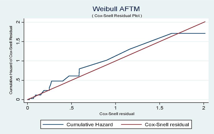
Figure 1 Cox Snell residual plot.

4 Discussion

In this study we have determined the significant predictors and their effects on the survival of endometrial cancer patients using AFTM. We have compared various frequently used AFTM viz. Exponential, Weibull, Log-logistic, Log-normal, Gompertz, Gamma and Generalized Gamma in our analysis. Besides, Exponential AFTM, all other model shows the similar value of Log-Likelihood, AIC and BIC value. Which means all the considered AFT models fits well and shows analogous result except Exponential AFTM. This result justifies our AFT model selection. Among these models based on the highest Log-Likelihood, lowest AIC and BIC value the Weibull AFTM was found to be the best fitted model for explaining the survival of Endometrial cancer patients with UPSC. Earlier Weibull AFTM was found to be best fitted AFTM for lymphoblastic leukemia patients (Sayehmiri et al., 2008). The Cox-Snell residual plot (Figure 1) revealed that the selected Weibull AFTM fits well for the endometrial cancer survival data.

In this study, we have observed that six covariates viz., age, isolated para-aortic status, PWPWD, comorbidities, tumor size and adnexa status are significantly associated with the survival of endometrial cancer patients (P $<$ 0.05). Whereas the other predictors grade, histology, cervical extension, myometrial invasion etc., are found as insignificant.

As expected, the relative survival is highly dependent on the age of diagnosis of endometrial cancer patients. The relative survival decreases with increasing age and this is also seen in other studies reported by Cook et al. (2006) and Elit et al. (2012). This may in part be related to higher rate of comorbidities in older women.

In this study, an increased tumor size is found to be significantly associated with poor survival of endometrial cancer patients. Which is consistent with the findings reported by Blackburn et al. (2019), that the patients with tumor size $>$2 cm is less likely to have survival than their counterpart. In addition, patients with comorbidities and post-menopausal watery discharge had poor survival.

To our knowledge, this is the first study of its kind in evaluating the survival characteristics of endometrial cancer patients with UPSC using different AFTM in the state of Odisha. Since UPSC is a rare category of endometrial cancer, the patients with poor prognosis and have been diagnosed at an advanced stage. Studies have explored the survival characteristics of advanced stage endometrial cancer (Goodman et al., 2019, Chen et al., 2020). Solmaz et al. (2016) found that LVSI was a significant covariate for the survival of endometrial cancer patients with UPSC but in our study we found it is not statistically significant.

It is worth here to mention the limitation of this study, the small sample size is the major limitation. Thus, the generalization of this study can be validated by taking a larger sample size and more number of covariates.

5 Conclusion

The findings of this study shows that Weibull AFT model was found as best fit model in explaining the determinants of survival of endometrial cancer patients with UPSC. The covariates like age, isolated para-aortic status, comorbidities, tumor size and adnexa status are significantly associated with the survival of patients. Considering this information, more importance can be given to the patients with such prognostic factors. Hence by optimizing different treatment based on such prognostic factors plays an important role in managing endometrial cancer at early stage.

References

[1] Ali, Z. A. R. E., Hosseini, M., Mahmoodi, M., Mohammad, K., Zeraati, H., and Naieni, K. H. (2015). A comparison between accelerated failure-time and Cox proportional hazard models in analyzing the survival of gastric cancer patients. Iranian journal of public health, 44(8), 1095.

[2] Baik, J., and Murthy, D. P. (2008). Reliability assessment based on two-dimensional warranty data and an accelerated failure time model. International Journal of Reliability and Safety, 2(3), 190–208.

[3] Blackburn, B. E., Soisson, S., Rowe, K., Snyder, J., Fraser, A., Deshmukh, V., Newman, M., Smith, K., Herget, K., Kirchhoff, A.C., Kepka, D., Werner, T.L., Gaffney, D., Mooney, K., and Hashibe, M. (2019). Prognostic factors for rural endometrial cancer patients in a population-based cohort. BMC public health, 19(1), 1–9.

[4] Bokoro, P., and Doorsamy, W. (2018). Reliability analysis of low-voltage metal-oxide surge arresters using accelerated failure time model. IEEE Transactions on Power Delivery, 33(6), 3139–3146.

[5] Bregar, A. J., Rauh-Hain, J. A., Spencer, R., Clemmer, J. T., Schorge, J. O., Rice, L. W., and Del Carmen, M. G. (2017). Disparities in receipt of care for high-grade endometrial cancer: a National Cancer Data Base analysis. Gynecologic oncology, 145(1), 114–121.

[6] Chapman, J. A. W., Trudeau, M. E., Pritchard, K. I., Sawka, C. A., Mobbs, B. G., Hanna, W. M., … and Lickley, L. A. (1992). A comparison of all-subset Cox and accelerated failure time models with Cox step-wise regression for node-positive breast cancer. Breast cancer research and treatment, 22(3), 263–272.

[7] Chen, H. H., Ting, W. H., Sun, H. D., Wei, M. C., Lin, H. H., and Hsiao, S. M. (2020). Predictors of Survival in Women with High-Risk Endometrial Cancer and Comparisons of Sandwich versus Concurrent Adjuvant Chemotherapy and Radiotherapy. International Journal of Environmental Research and Public Health, 17(16), 5941.

[8] Coll de la Rubia, E., Martinez-Garcia, E., Dittmar, G., Gil-Moreno, A., Cabrera, S., and Colas, E. (2020). Prognostic biomarkers in endometrial cancer: a systematic review and meta-analysis. Journal of clinical medicine, 9(6), 1900.

[9] Collett, D. (2015). Modelling survival data in medical research.3rd edition, London, UK, Chapman-Hall, CRC press.

[10] Cook, L. S., Kmet, L. M., Magliocco, A. M., and Weiss, N. S. (2006). Endometrial cancer survival among US black and white women by birth cohort. Epidemiology, 17(4), 469–472.

[11] Cox, D. R., and Snell, E. J. (1968). A general definition of residuals (with discussion). Journal of the Royal Statistical Society.

[12] Dessai, S. B., Adrash, D., Geetha, M., Arvind, S., Bipin, J., Nayanar, S., Sachin, K., Biji, M.S., and Balasubramanian, S. (2016). Pattern of care in operable endometrial cancer treated at a rural-based tertiary care cancer center. Indian journal of cancer, 53(3), 416.

[13] Elit, L., Lytwyn, A., and Akhtar-Danesh, N. (2012). Long-Term Trends in the Survival of Women with Endometrial Cancer in Canada: A Population-Based Study. Journal of Cancer Therapy, 3(05), 853.

[14] Goodman, C. R., Hatoum, S., Seagle, B. L. L., Donnelly, E. D., Barber, E. L., Shahabi, S. & Strauss, J. B. (2019). Association of chemotherapy and radiotherapy sequence with overall survival in locoregionally advanced endometrial cancer. Gynecologic oncology, 153(1), 41–48.

[15] Juhan, N., Abd Razak, N., Zubairi, Y. Z., Naing, N. N., Hussin, C. H. C., and Daud, M. A. (2016). Comparison of stratified Weibull model and Weibull accelerated failure time (aft) model in the analysis of cervical cancer survival. Jurnal Teknologi, 78(6–4).

[16] Kay, R., and Kinnersley, N. (2002). On the use of the accelerated failure time model as an alternative to the proportional hazards model in the treatment of time to event data: a case study in influenza. Drug information journal, 36(3), 571–579.

[17] Khanal, S. P., Sreenivas, V., and Acharya, S. K. (2014). Accelerated failure time models: an application in the survival of acute liver failure patients in India. Int J Sci Res, 3, 161–166.

[18] Klein, J. P., and Moeschberger, M. L. (1997). Survival Analysis: Techniques for Censored and Truncated Data. 1st Edition, Springer, New York.

[19] Lawless, J. F. (1982). Statistical models and methods for lifetime data, New Work. John Wiley.

[20] Lee, E. T., and Wang, J. (2003). Statistical methods for survival data analysis (Vol. 476). John Wiley & Sons.

[21] Miller, K. D., Siegel, R. L., Lin, C. C., Mariotto, A. B., Kramer, J. L., Rowland, J. H., Stein, K.D., Alteri, R., and Jemal, A. (2016). Cancer treatment and survivorship statistics, 2016. CA: a cancer journal for clinicians, 66(4), 271–289.

[22] Nicholas, Z., Hu, N., Ying, J., Soisson, P., Dodson, M., and Gaffney, D. K. (2014). Impact of comorbid conditions on survival in endometrial cancer. American journal of clinical oncology, 37(2), 131–134.

[23] Orbe, J., Ferreira, E., and Nunez-Anton, V. (2002). Comparing proportional hazards and accelerated failure time models for survival analysis. Statistics in medicine, 21(22), 3493–3510.

[24] Saikia, R., and Barman, M. P. (2017). Comparing accelerated failure time models with its specific distributions in the analysis of esophagus cancer patients’ data. International Journal of Computational and Applied Mathematics, 12(2), 411–424.

[25] Sayehmiri, K., Eshraghian, M. R., Mohammad, K., Alimoghaddam, K., Foroushani, A. R., Zeraati, H. and Ghavamzadeh, A. (2008). Prognostic factors of survival time after hematopoietic stem cell transplant in acute lymphoblastic leukemia patients: Cox proportional hazard versus accelerated failure time models. Journal of Experimental & Clinical Cancer Research, 27(1), 1–9.

[26] Schwarz, G. (1978). Estimating the dimension of a model. The annals of statistics, 461–464.

[27] Solmaz, U., Ekin, A., Mat, E., Gezer, C., Dogan, A., Biler, A. and Sanci, M. (2016). Analysis of clinical and pathological characteristics, treatment methods, survival, and prognosis of uterine papillary serous carcinoma. Tumori Journal, 102(6), 593–599.

[28] Srividhya, K., and Radhika, A. (2019). Comparison of Different Parametric Modeling for Time-to-Event Data Among Cancer Patients. International Journal of Scientific Research in Mathematical and Statistical Sciences, 6(1), 187–192.

[29] Swain, P. K., and Grover, G. (2016). Determination of predictors associated with HIV/AIDS patients on ART using accelerated failure time model for interval censored survival data. Am J Biostat, 6, 12–19.

[30] Wei, L. J. (1992). The accelerated failure time model: a useful alternative to the Cox regression model in survival analysis. Statistics in medicine, 11(14–15), 1871–1879.

Biographies

Manas Ranjan Tripathy, completed his master’s degree and the master in philosophy degree in Statistics from Ravenshaw University, Cuttack, Odisha in 2016 and 2017, respectively. He is a University Topper (gold medallist) in his master’s degree in statistics. He is currently a Ph.D Student at the Department of Statistics in Ravenshaw University, Cuttack, Odisha. His research area includes, Biostatistics and Demography.

Prafulla Kumar Swain, holds master degree from Banaras Hindu University, and Ph.D.(Statistics) from University of Delhi. Currently, he is working as Assistant Professor in Statistics at Utkal University, Bhubaneswar, India. He has published more than forty research papers in peer reviewed national and international reputed journals in the field of HIV/AIDS, Cancer epidemiology, maternal and child health. He is a University Topper (gold medallist) and won many awards/accolades in his academic career. He has been academic editor and reviewer for many reputed journals.

Pravat Kumar Sarangi, completed his Post Graduation in Statistics from Utkal University, Bhubaneswar, Odisha in 1984 and M.Phil from Meerut University, UP in 1986. He has done his Ph.D from Utkal University, Bhubaneswar, Odisha in 2007. His area of Research is Demography and Population Studies. He has published several research papers in different national and international journals.

S. S. Pattnaik, currently working as senior resident (LTMRO) at the Department of Gynaecology Oncology, AHRCC, Cuttack, Odisha. Her research specialisation is Oncology, Obstetrics, etc. She has published several research papers in different national and international journals.

Journal of Reliability and Statistical Studies, Vol. 15, Issue 2 (2022), 723–744.
doi: 10.13052/jrss0974-8024.15213
© 2023 River Publishers

Abstract

1 Introduction

2 Materials and Methods

2.1 Data Source

2.2 Methodology

2.3 Exponential AFTM

2.4 Weibull AFTM

2.5 Log-logistic AFTM

2.6 Log-normal AFTM

2.7 Gompertz AFTM

2.8 Gamma AFTM

2.9 Generalized Gamma AFTM

2.10 Maximum Likelihood Estimation of the parameters of AFTM

2.11 Model Selection Criteria

2.12 Model Checking Criteria

3 Analysis and Results

4 Discussion

5 Conclusion

References

Biographies