A Semi-parametric NHPP-based Software Reliability Modeling with Local Polynomial Debug Rate

Siqiao Li^*, Tadashi Dohi and Hiroyuki Okamura

Graduate School of Advanced Science and Engineering, Hiroshima University, Higashi-Hiroshima, Japan
E-mail: rel-siqiao@hiroshima-u.ac.jp; dohi@hiroshima-u.ac.jp; okamu@hiroshima-u.ac.jp
*Corresponding Author

Received 11 November 2021; Accepted 09 February 2022; Publication 31 March 2023

Abstract

In this paper, we propose a new non-homogeneous Poisson process (NHPP) based software reliability model (SRM), where the software debug rate is given by a local polynomial function. The main feature of this semi-parametric SRM is to control the goodness-of-fit by changing the polynomial degree. Numerical examples with 16 actual software development project data are devoted to comparing our SRM with the well-known existing NHPP-based SRMs in terms of goodness-of-fit and predictive performances.

Keywords: Software reliability models, non-homogeneous Poisson processes, semi-parametric approach, local polynomial debug rate, maximum likelihood estimation, goodness-of-fit performance, predictive performance.

1 Introduction

While the software has become the key information platform in every computer-based system, the size and complexity have increased accordingly. Thus, software reliability has received much attention as the most important attribute in software quality. In the past few decades, many software reliability models (SRMs) have been proposed to describe software fault-detection processes and assess the software reliability quantitatively. Among them, the most popular SRMs are the non-homogeneous Poisson process-based (NHPP)-based SRMs, which can be characterized by the software fault-detection time distribution. In other words, the existing NHPP-based SRMs are described with the representative software fault-detection time distribution functions. Since the seminal contribution by Goel and Okumoto [5], several SRMs have assumed the well-known continuous probability distribution functions such as Pareto distribution [1], log-normal distribution [2], exponential distribution [5], Weibull distribution [6], log-logistic distribution [7], truncated logistic distribution [13], gamma distribution [20, 22], extreme distributions including Gompertz distribution [14], truncated normal distribution [16]. Okamura and Dohi [17] implemented the above 11 SRMs in software reliability assessment tool on spreadsheet, SRATS.

However, practical experiences suggest no unique SRM that could fit every software fault-count data, so in parametric software reliability modeling, selection of fault-detection time distribution is always needed. In this paper, we propose a new NHPP-based SRM, where the software debug rate is given by a local polynomial function. The fundamental idea comes from the assumption that the software debug rate, which is equivalent to the hazard rate function of software fault-detection time distribution, is approximated by an arbitrary polynomial function. This intuitive but well-motivated assumption seems reasonable because one does not need to select a parametric form of the probability distribution function. The main feature of this semi-parametric SRM is to control the goodness-of-fit by changing the polynomial degree. We determine the polynomial degree by the well-known Akaike information criterion (AIC) and select the best local polynomial debug rate. It is worth mentioning that this kind of semi-parametric SRM has not been proposed during the last four decades. Recently, Nafreen and Fiondella [12] were concerned about the software debug rate and overviewed several NHPP-based SRMs with bathtub-shaped debug rate. Especially, they dealt with a low-order polynomial function called the quadratic model. We show that their model is a special case of our semi-parametric SRM and that the low order polynomial function is not enough to guarantee satisfactory goodness-of-fit performance compared with the existing parametric models [17].

The remaining part of this paper is organized as follows. In Section 2, we summarize the NHPP-based SRMs. Section 3 describes the polynomial software debug rate and proposes our semi-parametric SRMs. In Section 4, we overview the maximum likelihood estimation for the NHPP-based SRMs, where two kinds of software fault-count data; time-domain data and time-interval (group) data. It should be noted that the parameter estimation of our semi-parametric NHPP-based SRM with local polynomial debug rate is not so trivial because the maximum likelihood estimation has to be made with a constraint that the software debug rate is non-negative. In Section 5, numerical examples with 16 actual software development project data are devoted to comparing our SRM with the well-known existing NHPP-based SRMs in terms of goodness-of-fit and predictive performances. Finally, the paper is concluded with some remarks in Section 6.

2 NHPP-based Software Reliability Modeling

Let $N(t)$ be the cumulative number of software faults detected by time $t(\ge 0)$. The stochastic point process $N(t)$ is said a non-homogeneous Poisson process (NHPP) if the probability mass function (PMF), $P_n(t)=\mathrm{Pr}\{N(t)=n|N(0)=0\}$, is given by

$$P_n(t)=\frac{{\{\mathrm{\Lambda }(t;\mathit{\theta })\}}^n}{n!}\exp (-\mathrm{\Lambda }(t;\mathit{\theta })),n=0,1,2,\mathrm{\dots },$$

(1)

where $\mathrm{\Lambda }(t;\mathit{\theta })$ is called the mean value function, which denotes the expected cumulative number of software faults by time $t$;

$$\text{E}[N(t)]=\mathrm{\Lambda }(t;\mathit{\theta })={\int }_0^t\lambda (x;\mathit{\theta })\mathit{d}x$$

(2)

with the intensity function $\lambda (t;\mathit{\theta })$ and the model parameter vector $\mathit{\theta }$.

Once the mean value function or the intensity function was given, it is possible to characterize the PMF of NHPP in Equation (1). Instead, Yamada and Osaki [21] characterized the NHPP-based SRMs with the software debug rate. Let

$d(t;\mathit{\alpha })=\lambda (t;\mathit{\theta })/\{\omega -\mathrm{\Lambda }(t;\mathit{\theta })\}$

(3)

be the software debug rate, where $\mathit{\theta }=(\omega ,\mathit{\alpha })$, $\omega ={lim}_{t\to \mathrm{\infty }}\mathrm{\Lambda }(t;\mathit{\theta })$. It is evident that $d(t;\mathit{\alpha })$ implies the instantaneous fault detection rate per expected remaining faults. Also, it is immediate to see that Equation (3) is rewritten as

${\displaystyle \frac{d\mathrm{\Lambda }(t;\mathit{\theta })}{dt}}=d(t;\mathit{\alpha })\{\omega -\mathrm{\Lambda }(t;\mathit{\theta })\}.$

(4)

In the NHPP-based software reliability modeling, it is common to assume that the mean value function is bounded, i.e., $\mathrm{\Lambda }(t;\mathit{\theta })=\omega F(t;\mathit{\alpha })$, where $\omega (>0)$ denotes the mean number of inherent software faults before software testing, and $F(t;\mathit{\alpha })$ is an arbitrary continuous cumulative distribution function (CDF). Then, it is seen that $\mathrm{\Lambda }(t;\mathit{\theta })=\omega F(t;\mathit{\alpha })$ if and only if $d(t;\mathit{\alpha })=f(t;\mathit{\alpha })/\{1-F(t;\mathit{\alpha })\}$ with the probability density function (PDF) $f(t;\mathit{\alpha })=dF(t;\mathit{\alpha })/dt$. Hence, the software debug rate is equivalent to the hazard rate of the fault-detection time CDF $F(t;\mathit{\alpha })$.

Table 1 The existing NHPP-based SRMs

Models	$\mathrm{\Lambda }(t;\mathit{\theta })$	$d(t;\mathit{\alpha })$
Exponential dist.	(exp) [5]	$\mathrm{\Lambda }(t;\mathit{\theta })=\omega F(t;\mathit{\alpha })$	$F(t;\mathit{\alpha })=1-e^{-bt}$	$d(t;\mathit{\alpha })=b$
Gamma dist.	(gamma) [20],[22]	$\mathrm{\Lambda }(t;\mathit{\theta })=\omega F(t;\mathit{\alpha })$	$F(t;\mathit{\alpha })={\int }_0^t\frac{c^b{s}^{b-1}{e}^{-cs}}{\mathrm{\Gamma }(b)}\mathit{d}s$	$d(t;\mathit{\alpha })=\frac{c^b{t}^{b-1}{e}^{-ct}}{\mathrm{\Gamma }(b)-{\int }_0^t{s}^{b-1}{e}^{-cs}\mathit{d}s}$
Pareto dist.	(pareto) [1]	$\mathrm{\Lambda }(t;\mathit{\theta })=\omega F(t;\mathit{\alpha })$	$F(t;\mathit{\alpha })=1-{(\frac{b}{t+b})}^c$	$d(t;\mathit{\alpha })=\frac{b}{c+t}$
Truncated normal dist.	(tnorm) [16]	$\mathrm{\Lambda }(t;\mathit{\theta })=\omega \frac{F(t;\mathit{\alpha })-F(0;\mathit{\alpha })}{1-F(0;\mathit{\alpha })}$	$F(t;\mathit{\alpha })=\frac{1}{\sqrt{2\pi }b}{\int }_{-\mathrm{\infty }}^t{e}^{-\frac{{(s-c)}^2}{2b^2}}\mathit{d}s$	$d(t;\mathit{\alpha })=-\frac{\sqrt{\frac{2}{\pi }}{e}^{-\frac{{(c-t)}^2}{2b^2}}}{b\left(\text{erfc}\left(\frac{c-t}{\sqrt{2}b}\right)-2\right)}$	$\text{erfc}\left(\frac{c-t}{\sqrt{2}b}\right)=1-\frac{2}{\sqrt{\pi }}{\int }_0^{\frac{c-t}{\sqrt{2}b}}{e}^{-s^2}\mathit{d}s$
Log-normal dist.	(lnorm) [2],[16]	$\mathrm{\Lambda }(t;\mathit{\theta })=\omega F(\ln t;\mathit{\alpha })$	$F(t;\mathit{\alpha })=\frac{1}{\sqrt{2\pi }b}{\int }_{-\mathrm{\infty }}^t{e}^{-\frac{{(s-c)}^2}{2b^2}}\mathit{d}s$	$d(t;\mathit{\alpha })=\frac{\sqrt{\frac{2}{\pi }}{e}^{-\frac{{(c-\log (t))}^2}{2b^2}}}{bt\left(\text{erfc}\left(\frac{c-\log (t)}{\sqrt{2}b}\right)-2\right)}$	$\text{erfc}\left(\frac{c-\log (t)}{\sqrt{2}b}\right)=1-\frac{2}{\sqrt{\pi }}{\int }_0^{\frac{c-\log (t)}{\sqrt{2}b}}{e}^{-s^2}\mathit{d}s$
Truncated logistic dist.	(tlogist) [13]	$\mathrm{\Lambda }(t;\mathit{\theta })=\omega F(t;\mathit{\alpha })$	$F(t;\mathit{\alpha })=\frac{1}{1+e^{-\frac{t-c}{b}}}$	$d(t;\mathit{\alpha })=\frac{e^{t/b}}{b{e}^{c/b}+b{e}^{t/b}}$
Log-logistic dist.	(llogist) [7]	$\mathrm{\Lambda }(t;\mathit{\theta })=\omega F(\ln t;\mathit{\alpha })$	$F(t;\mathit{\alpha })=\frac{1}{1+e^{-\frac{t-c}{b}}}$	$d(t;\mathit{\alpha })=\frac{t^{\frac{1}{b}-1}}{b\left(e^{c/b}+t^{1/b}\right)}$
Truncated extreme-value max dist.	(txvmax) [14]	$\mathrm{\Lambda }(t;\mathit{\theta })=\omega \frac{F(t;\mathit{\alpha })-F(0;\mathit{\alpha })}{1-F(0;\mathit{\alpha })}$	$F(t;\mathit{\alpha })=e^{-e^{-\frac{t-c}{b}}}$	$d(t;\mathit{\alpha })=\frac{e^{\frac{c-t}{b}}}{b\left(e^{e^{\frac{c-t}{b}}}-1\right)}$
Log-extreme-value max dist.	(lxvmax) [14]	$\mathrm{\Lambda }(t;\mathit{\theta })=\omega F(\ln t;\mathit{\alpha })$	$F(t;\mathit{\alpha })=e^{-e^{-\frac{t-c}{b}}}$	$d(t;\mathit{\alpha })=\frac{e^{c/b}{t}^{-\frac{b+1}{b}}}{b\left(e^{e^{c/b}{t}^{-1/b}}-1\right)}$
Truncated extreme-value min dist.	(txvmin) [14]	$\mathrm{\Lambda }(t;\mathit{\theta })=\omega \frac{F(0;\mathit{\alpha })-F(t;\mathit{\alpha })}{F(0;\mathit{\alpha })}$	$F(t;\mathit{\alpha })=e^{-e^{-\frac{t-c}{b}}}$	$d(t;\mathit{\alpha })=\frac{e^{\frac{c+t}{b}}}{b}$
Log-extreme-value min dist.	(lxvmin) [6]	$\mathrm{\Lambda }(t;\mathit{\theta })=\omega \left(1-F(-\ln t;\mathit{\alpha })\right)$	$F(t;\mathit{\alpha })=e^{-e^{-}\frac{t-c}{b}}$	$d(t;\mathit{\alpha })=\frac{e^{c/b}{t}^{\frac{1}{b}-1}}{b}$
$\left(\omega >0,a>0,b>0,c>0\right)$

Okamura and Dohi [17] implemented the existing NHPP-based SRMs with 11 software fault-detection time CDFs in the software reliability assessment tool on the spreadsheet (SRATS), which includes exponential (exp), gamma, Pareto, log-normal (lnorm), log-logistic (llogist), log-extreme-value minimum (lxvmin), log-extreme-value maximum (lxvmax), truncated logistic (tlogist), truncated normal (tnorm), truncated extreme-value minimum (txvmin), truncated extreme-value maximum (txvmax) distributions. In Table 1, we summarize these 11 NHPP-based SRMs.

3 Polynomial Software Debug Rate

Probability distributions with a polynomial hazard rate function have been used for modeling lifetimes in reliability engineering. Lawless [8] gave some examples of the least-squares estimation and the maximum likelihood estimation for the basic polynomial hazard rate model and their variants with censoring and grouped data. Csenki [4] derived the Laplace transform of the continuous random variable with a local polynomial hazard rate function and applied it to estimate the polynomial coefficients from the sample moments of the CDF.

Suppose that

$$d(t;\mathit{\alpha })={\mu }_0+{\mu }_{1}t+{\mu }_2{t}^2+\mathrm{\cdots }+{\mu }_m{t}^m,$$

(5)

where $\mathit{\alpha }=({\mu }_0,{\mu }_1,\mathrm{\dots },{\mu }_m)\in$ ${ℝ}^{m+1}$. Then the CDF is expressed as

$$F(t;\mathit{\alpha })=1-\exp \left(-\sum _{j=0}^m\frac{{\mu }_j{t}^{j+1}}{j+1}\right).$$

(6)

The above CDF with $m+1$ degrees is interpreted as a probability model on the minimum of $m+1$ independent Weibull random variables if $\mathit{\alpha }\in {ℝ}_{+}^{m+1}$, where $j$-th of them has scale parameter ${}^{j+1}\sqrt{(j+1)/{\mu }_j}$ and shape parameter $j+1$.

As special cases, when $m=0$ and $m=1$, the hazard rate functions become $d(t;\mathit{\alpha })={\mu }_0$ and $d(t;\mathit{\alpha })={\mu }_0+{\mu }_{1}t$, respectively. Balakrishnan and Malik [3], Mahmoud and Al-Nagar [10] called the latter probability model the linear exponential distribution. Nafreen and Fiondella [12] considered an NHPP-based SRM with the linear exponential distribution for the purpose to develop a bathtub-shaped debug rate. Hence, it is evident that Equation (5) is a general form to express the software debug rate.

If we assume that $\mathit{\alpha }\in {ℝ}_{+}^{m+1}$, i.e., $({\mu }_0,{\mu }_1,\mathrm{\dots },{\mu }_m)$ are all positive real numbers, it always holds that $d(t;\mathit{\alpha })\ge 0$ and $F(t;\mathit{\alpha })$ is increasing hazard rate (IHR). However, dissimilar to hardware reliability, it is well known that the software reliability growth phenomenon can be observed in software testing. In other words, the IHR assumption seems to be rather strong and not to be plausible to explain the software reliability growth. Hence the polynomial parameters may be negative except for ${\mu }_0$, because ${\mu }_0\ge 0$ is a necessary condition of $d(t;\mathit{\alpha })\ge 0$. In fact, it is not so easy to find out $\mathit{\alpha }\in {ℝ}^m$ with ${\mu }_0\ge 0$ to satisfy $d(t;\mathit{\alpha })\ge 0$. In the next section, we develop a somewhat heuristic, but exact maximum likelihood estimation method for our semi-parametric SRM with a local polynomial software debug rate with order $m$.

4 Maximum Likelihood Estimation

Maximum likelihood (ML) estimation is a commonly utilized method for the parameter estimation of NHPP-based SRMs. In ML estimation, the estimates are given by the parameters maximizing the log-likelihood function. On the other hand, the Maximum log-likelihood (MLL) depends on the observed data as well as the underlying NHPP-based SRMs. In this paper, two types of data; time-domain data and time-interval data (group data) are considered. Suppose that $k$ software faults are detected at testing time sequence $\{t_1,t_2,\mathrm{\dots },t_k\}$, so, the likelihood function is represented as

$\text{L}(\mathit{\theta })=\text{exp}(-\mathrm{\Lambda }(t_k;\mathit{\theta })){\displaystyle \prod _{i=1}^k}\lambda (t_i;\mathit{\theta }),$

(7)

and the log-likelihood function can be written by

$\text{ln}\text{L}(\mathit{\theta })={\displaystyle \sum _{i=1}^k}\ln \lambda (t_i;\mathit{\theta })-\mathrm{\Lambda }(t_k;\mathit{\theta }).$

(8)

Next, consider the case where the group data, $(t_i,n_i)$, are observed. A group data consists of the number of faults detected in fixed time intervals measured with the calendar time, $(t_{i-1},t_i](i=1,2,\mathrm{\dots },k)$. The likelihood function is given by

$\text{L}(\mathit{\theta })={\displaystyle \prod _{i=1}^k}\left[{\displaystyle \frac{{[\mathrm{\Lambda }(t_i;\mathit{\theta })-\mathrm{\Lambda }(t_{i-1};\mathit{\theta })]}^{n_i-n_{i-1}}}{(n_i-n_{i-1})!}}\right]\times e^{-[\mathrm{\Lambda }(t_i;\mathit{\theta })-\mathrm{\Lambda }(t_{i-1};\mathit{\theta })]},$

(9)

where $t_i$ is the observation time and $n_i$ is the cumulative number of software faults detected by time $t_i$.

Then, the log-likelihood function can be written by

$\text{ln}\text{L}(\mathit{\theta })$	$={\displaystyle \sum _{i=1}^k}(n_i-n_{i-1})\ln \{\mathrm{\Lambda }(t_i;\mathit{\theta })-\mathrm{\Lambda }(t_{i-1};\mathit{\theta })\}$
	$\mathrm{\hspace{1em}}-{\displaystyle \sum _{i=1}^k}\ln \{(n_i-n_{i-1})!\}-\mathrm{\Lambda }(t_m;\mathit{\theta }).$	(10)

Then the maximum likelihood (ML) estimate $\widehat{\mathit{\theta }}\in (\widehat{\omega },\widehat{\mathit{\alpha }})$ can be obtained as a solution of ${\mathrm{argmax}}_{\mathit{\theta }}\text{ln}\text{L}(\mathit{\theta })$ in Equation (8) and Equation (10), subject to $d(t_i,\widehat{\mathit{\alpha }})={\widehat{\mu }}_0+{\widehat{\mu }}_1{t}_i+{\widehat{\mu }}_2{t}_i^2+\mathrm{\cdots }+{\widehat{\mu }}_m{t}_i^m\ge 0$ with $i=1,2,\mathrm{\dots },k$. In what follows, we consider two cases;

• Case I: $\mathit{\alpha }=({\mu }_0,{\mu }_1,\mathrm{\dots },{\mu }_m)\in {ℝ}_{+}^{m+1}$ are all positive real numbers.

• Case II: ${\mu }_0\ge 0$ and $({\mu }_1,\mathrm{\dots },{\mu }_m)\in {ℝ}^m$ are real numbers.

It is obvious that Case I is restrictive because the software debug rate is always increasing in time $t$. However, the maximum likelihood estimation is easily made because of $d(t_i,\widehat{\mathit{\alpha }})\ge 0$ for all the observation data $t_i(i=1,2,\mathrm{\dots },k)$. In Case II, we consider all the combinations of ${\mu }_j\in {ℝ}_{+}$ and ${\mu }_j\in {ℝ}_{-}$ for all $j=1,2,\mathrm{\dots },m$, say $2^m$ combinations and solve the maximization problems with constraint $d(t_i,\mathit{\alpha })\ge 0$. Note that the general-purpose optimization solver such as Mathematica and MATLAB enables to solve the above problem when the search space for each polynomial coefficient is limited in the positive or negative region. Figures 1 and 2 illustrate the behaviors of our polynomial debug rates $d(t_i,\widehat{\mathit{\alpha }})$ with degree $m=1,2,\mathrm{\dots },6$ in time-domain data (TDS1) of Table 2 and group data set (GDS1) of Table 3 in Case I. It is seen that all the software debug rates are increasing in time. On one hand, in Figures 3 and 4, we plot the behaviors of software debug rates with TDS1 and GDS1, respectively, in Case II. As the polynomial degree $m$ increases, the polynomial software debug rates fluctuate and can represent much more complex behaviors. It is possible to represent the non-increasing behaviors of software debug rate by relaxing the assumption of $\mathit{\alpha }\in {ℝ}_{+}^{m+1}$ and to increase the log-likelihood function as well. Note that our purpose is not to compare Case I with Case II, because Case I is involved as a special case of Case II. We aim at investigating the estimation effect between Case I and Case II, and comparing our semi-parametric NHPP-based SRM with the existing parametric NHPP-based SRMs.

5 Numerical Examples

5.1 Data Sets

In numerical experiments, we chose 8 software fault-detection time-domain (TDS1$\sim$TDS8) data in Table 2, measured with CPU time, and 8 software fault-detection group data (GDS1$\sim$GDS8) in Table 3, which consist of the number of software faults detected by each calendar time.

Table 2 Time-domain data sets

Data	No. faults	Source
TDS1	54	SYS2 [11]
TDS2	38	SYS3 [11]
TDS3	136	SYS1 [11]
TDS4	53	SYS4 [11]
TDS5	73	Project J5 [9]
TDS6	38	S10 [11]
TDS7	41	S27 [11]
TDS8	101	S17 [11]

Table 3 Group data sets

Data	No. Faults	Testing Periods	Source
GDS1	54	17	SYS2 [11]
GDS2	38	14	SYS3 [11]
GDS3	120	19	Release2 [19]
GDS4	61	12	Release3 [19]
GDS5	9	14	NASA-supported project [18]
GDS6	66	20	DS1 [15]
GDS7	58	33	DS2 [15]
GDS8	52	30	DS3 [15]

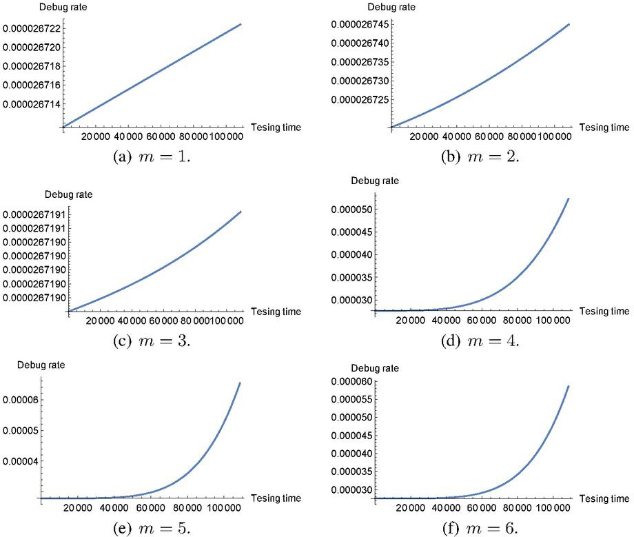
Figure 1 Behavior of software debug rates with TDS1 in Case I.

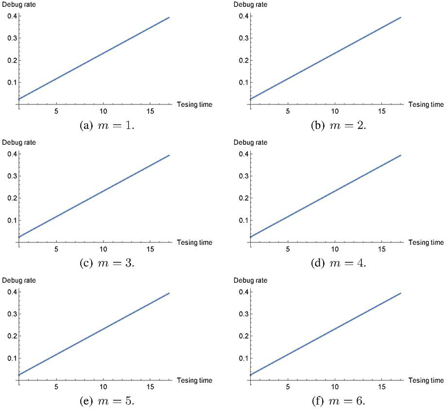
Figure 2 Behavior of software debug rates with GDS1 in Case I.

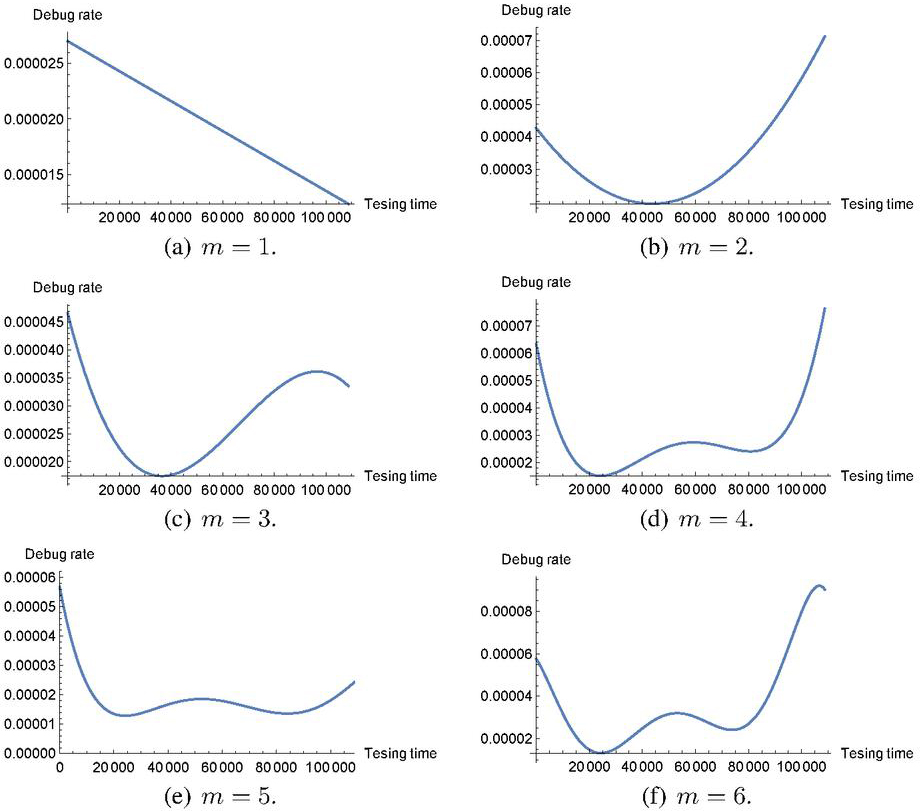
Figure 3 Behavior of software debug rates with TDS1 in Case II.

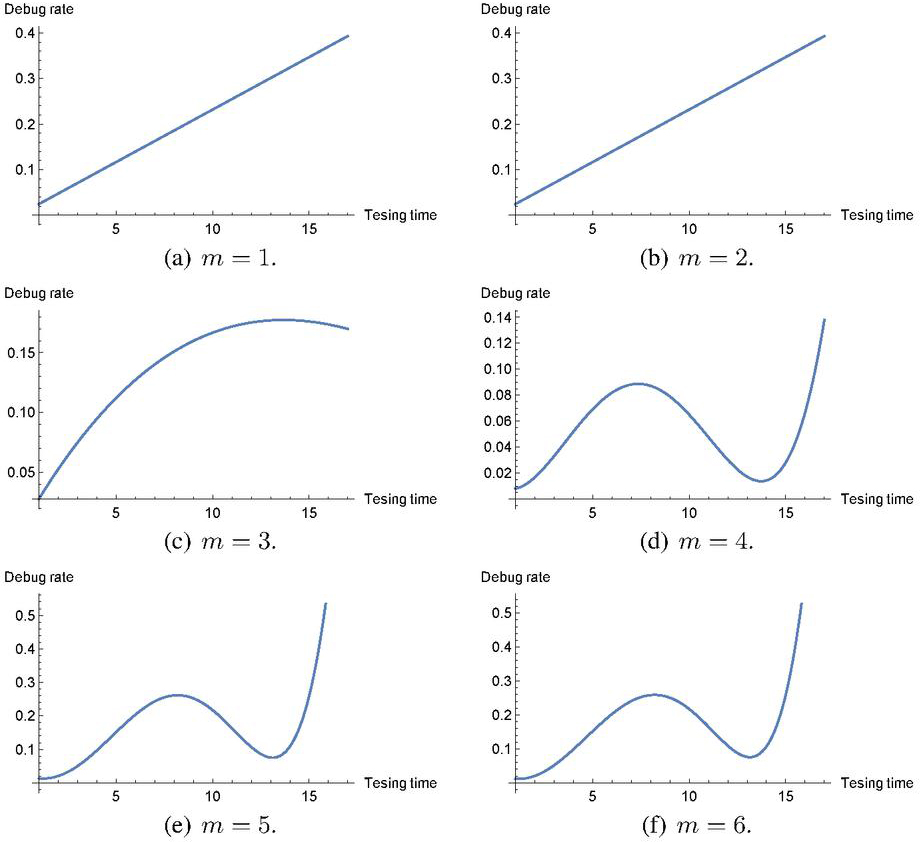
Figure 4 Behavior of software debug rates with GDS1 in Case II.

We derive the ML estimates of the model parameters, $\widehat{\mathit{\theta }}$, for our NHPP-based SRM with local polynomial debug rate, where the polynomial degree $m$ changes as the integer values $m=1,2,\mathrm{\dots }$, and compare them with the other 11 representative NHPP-based SRMs shown in Table 1.

5.2 Goodness-of-fit Performance

Define the following goodness-of-fit criteria:

• Maximum log-likelihood (MLL): $\ln \text{L}(\widehat{\mathit{\theta }})$

• Akaike information criterion (AIC):

$$\text{AIC}=-2\ln \text{L}(\widehat{\mathit{\theta }})+2\times (\text{the number of parameters})$$

(11)

• Mean squares error (MSE):

$$\text{MSE}(\widehat{\mathit{\theta }})=\frac{\sqrt{{\sum }_{i=1}^k{(n_i-\mathrm{\Lambda }(t_i;\widehat{\mathit{\theta }}))}^2}}{k}.$$

(12)

The smaller AIC/MSE represents the better SRM in terms of goodness-of-fit performances.

Figure 5 presents the mean value functions and the cumulative number of software faults detected in TDS1 and GDS1. The best SRMs with minimum AIC were selected from NHPP-based SRMs with local polynomial debug rate $(m=1,2,\mathrm{\dots },6)$ in both Case I and Case II (blue- and black-colored curves), and compared with the best existing NHPP-based SRMs in SRATS (orange-colored curve) in terms of AIC. At the first look, our semi-parametric NHPP-based SRMs could show more accurate estimations close to actual software fault counts. In Tables 4 and 5, we present the goodness-of-fit results of our semi-parametric NHPP-based SRMs with local polynomial debug rate in terms of AIC/MSE, where the polynomial degree $m$ changed from $1$ to $6$, and the best SRMs were based on the minimum AIC. From Table 4, it can be seen that our semi-parametric NHPP-based SRM in Case II could provide the smaller MLL and MSE than the existing SRATS NHPP-based SRMs in 5 time-domain data sets (TDS2, TDS5, TDS6, TDS7, and TDS8) and 3 time-domain data sets (TDS5, TDS7, and TDS8), respectively.

In the group data analysis, we found the minimum MLL and MSE in 6 out of 8 data sets (GDS1, GDS2, GDS3, GDS4, GDS6, and GDS7), so our semi-parametric NHPP-based SRM in Case II gave the minimum MLL and MSE. In GDS1, GDS4, and GDS6, it could provide the smaller AIC than the SRATS NHPP-based SRMS, even if the number of free parameters i n our semi-parametric SRMs is much larger than the representative SRMs in Table 1. We also notice that as the polynomial degree increases, the number of free parameters also increases, and that our semi-parametric SRMs with high-degree of polynomials could not always lead to the smaller AIC results. In fact, we confirmed the AIC values with $m=7,8,\mathrm{\dots }$ in our preliminary experiments and that $m=6$ is enough as the maximum polynomial degree from the viewpoint of minimization of AIC. In both tables, we evaluated MSE, which is a vertical distance between the mean value function and the underlying fault count data. It is clear that our semi-parametric SRMs tend to give larger MSE than the SRATS NHPP-based SRMs in 11 out of 16 data sets.

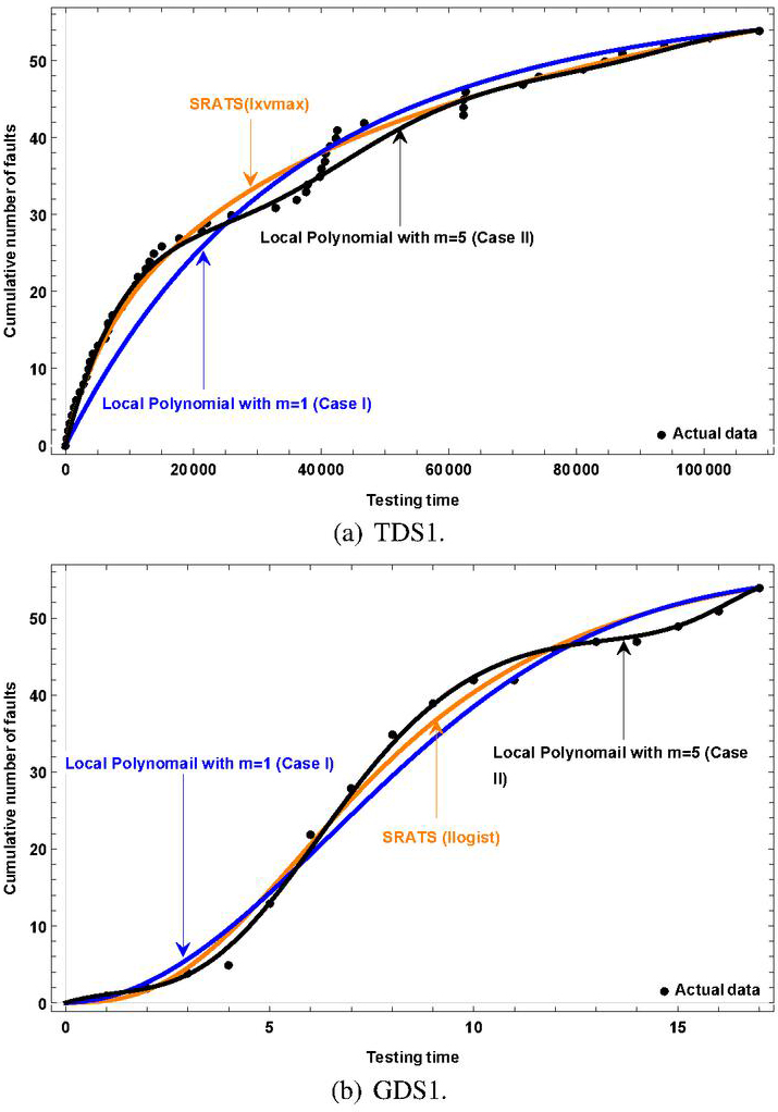
Figure 5 Behavior of cumulative number of software faults with SRMs.

Table 4 Goodness-of-fit results with time-domain data

	Semi-parametric SRM	SRATS
	Case I: $\mathit{\alpha }=({\mu }_0,{\mu }_1,\mathrm{\dots },{\mu }_m)\in {ℝ}_{+}^{m+1}$	Case II: ${\mu }_0\ge 0,({\mu }_1,\mathrm{\dots },{\mu }_m)\in {ℝ}^m$	$\mathit{\alpha }=(\omega ,a,b,c)\in {ℝ}_{+}$
	MLL	AIC	MSE	MLL	AIC	MSE	MLL	AIC	MSE
TDS1	$-$448.577	903.155 ($m=1$)	0.502	$-$446.589	901.177 ($m=2$)	0.282	$-$445.333	896.666 (lxvmax)	0.190
TDS2	$-$304.214	614.428 ($m=1$)	0.852	$-$294.511	601.022 ($m=4$)	0.194	$-$296.066	598.131 (lxvmax)	0.211
TDS3	$-$974.807	1955.610 ($m=1$)	0.711	$-$967.561	1943.120 ($m=2$)	0.227	$-$966.080	1938.160 (lxvmin)	0.220
TDS4	$-$377.974	761.948 ($m=1$)	0.319	$-$377.095	760.189 ($m=1$)	0.265	$-$376.878	759.756 (pareto)	0.267
TDS5	$-$376.870	759.740 ($m=1$)	0.522	$-$366.886	748.734 ($m=5$)	0.314	$-$376.935	757.869 (exp)	0.510
TDS6	$-$360.839	727.678 ($m=1$)	0.255	$-$360.839	727.678 ($m=1$)	0.255	$-$357.964	721.928 (lxvmax)	0.195
TDS7	$-$502.670	1011.340 ($m=1$)	0.579	$-$499.786	1007.570 ($m=2$)	0.354	$-$501.110	1008.220 (lxvmax)	0.382
TDS8	$-$1281.920	2569.830 ($m=1$)	1.942	$-$1231.38	2474.760 ($m=4$)	0.347	$-$1252.085	2504.170 (pareto)	0.685

Table 5 Goodness-of-fit results with group data

	Semi-parametric SRM	SRATS
	Case I: $\mathit{\theta }=({\mu }_0,{\mu }_1,\mathrm{\dots },{\mu }_m)\in {ℝ}_{+}^{m+1}$	Case II: ${\mu }_0\ge 0,({\mu }_1,\mathrm{\dots },{\mu }_m)\in {ℝ}^m$	$\mathit{\theta }=(\omega ,a,b,c)\in {ℝ}_{+}$
	MLL	AIC	MSE	MLL	AIC	MSE	MLL	AIC	MSE
GDS1	$-$35.367	76.735 ($m=1$)	0.698	$-$29.188	72.377 ($m=5$)	0.264	$-$33.527	73.053 (llogist)	0.492
GDS2	$-$29.485	64.969 ($m=1$)	0.464	$-$26.546	63.091 ($m=3$)	0.387	$-$27.847	61.694 (lxvmax)	0.481
GDS3	$-$40.858	87.715 ($m=1$)	0.646	$-$37.739	87.478 ($m=4$)	0.326	$-$40.634	87.267 (tnorm)	0.569
GDS4	$-$21.790	51.581 ($m=2$)	0.364	$-$21.320	50.639 ($m=2$)	0.265	$-$22.526	51.052 (tlogist)	0.405
GDS5	$-$12.736	31.472 ($m=1$)	0.096	$-$12.736	31.472 ($m=1$)	0.096	$-$12.956	29.911 (exp)	0.092
GDS6	$-$50.092	114.184 ($m=5$)	0.964	$-$45.257	100.514 ($m=3$)	0.644	$-$51.416	108.831 (lxvmax)	1.061
GDS7	$-$61.848	127.612 ($m=3$)	0.256	$-$57.676	125.351 ($m=3$)	0.235	$-$58.633	123.265 (txvmin)	0.253
GDS8	$-$60.971	129.942 ($m=2$)	0.757	$-$59.563	127.126 ($m=2$)	0.711	$-$55.735	117.470 (llogist)	0.532

5.3 Predictive Performances

It is worth mentioning that the better goodness-of-fit to the past observation does not always lead to the better performance for the future prediction. Since assessing the quantitative software reliability predicts the fault-free probability during a future testing/operational period, it is important to investigate the predictive performance of the NHPP-based SRMs with local polynomial debug rate. When $k$ and $n_k$ software fault counts data are available and that the prediction length is given by $l(=1,2,\mathrm{\dots })$, we use the predictive mean squared error (PMSE):

$\text{PMSE}(\widehat{\mathit{\theta }})$	$={\displaystyle \frac{\sum _{i=k+1}^{k+l}{\{i-\mathrm{\Lambda }(t_i;\widehat{\mathit{\theta }})\}}^2}{l}},$	(13)
$\text{PMSE}(\widehat{\mathit{\theta }})$	$={\displaystyle \frac{\sum _{i=k+1}^{k+l}{\{n_i-\mathrm{\Lambda }(t_i;\widehat{\mathit{\theta }})\}}^2}{l}},$	(14)

for the time-domain data and group data, respectively, where $\widehat{\mathit{\theta }}$ is the ML estimate with constraint $d(t_i,\mathit{\alpha })\ge 0$ with $(i=1,2,\mathrm{\dots },k,\mathrm{\dots },k+l)$. We set the observation point $k$ at 20%, 50% and 80% points of the whole time series data. That is, we predict the future behavior of the software fault count at $t_{k+1},t_{k+2},\mathrm{\dots },t_{k+l}$ from the training data; $t_1,t_2,\mathrm{\dots },t_k$ for the time-domain data and group data.

Tables 6 present the prediction results at each observation point based on the minimum PMSE in time-domain data sets, where we select the best SRM with the smallest PMSE from NHPP-based SRMs with local polynomial debug rate $(m=1,2,\mathrm{\dots },6)$ in both Case I and Case II, and the existing NHPP-based SRMs in SRATS. It is seen that, when the testing phase is early (20%), our semi-parametric NHPP-based SRM in Case I could provide the smaller PMSE than the existing SRATS NHPP-based SRMs in 2 time-domain data sets (TDS5 and TDS6). When the testing phase is middle (50%), our semi-parametric NHPP-based SRM in Case I tended to give the better predictive performance in 3 cases of time-domain data sets (TDS1, TDS4 and TDS8) and Case II could provide the smaller PMSE in TDS4. When the testing phase is latee (80%), our semi-parametric NHPP-based SRM in Case I outperformed the existing NHPP-based SRMs in SRATS in only TDS4 and TDS5.

In Table 7, we summarize the minimum PMSE with the group data, it can be pointed that the our semi-parametric NHPP-based SRM provided the smallest PMSE in some cases; i.e., 2 cases out of 8 group data sets in (i), 2 cases out of 8 group data sets in (ii) and 5 cases out of 8 group data sets in (iii).

In both time-domain and group data sets, when we compare the PMSE between our semi-parametric NHPP-based SRM in Case I and in Case II, we can observe that Case I and Case II could provide the same PMSEs in some cases; i.e., in Table 6, 5 cases out of 8 time-domain data sets in (i), 2 cases out of 8 time-domain data sets in (ii) and 1 case out of 8 time-domain data sets in (iii). In Table 7, 3 cases out of 8 group data sets in (i) and 2 cases out of 8 group data sets in (iii). It means that, regardless of Case I or Case II, the model parameters $\widehat{\mathit{\theta }}$ derived by ML estimation are all positive, says, $\widehat{\mathit{\theta }}\in {ℝ}_{+}^{m+1}$, and could provide the minimum PMSE, where the polynomial degree $m$ changed from $1$ to $6$. As we emphasized in Chapter 4, Case I is involved as a special case of Case II.

Table 6 Predictive results with time-domain data

	Semi-parametric SRM				SRATS
	Case I: $\mathit{\alpha }=({\mu }_0,{\mu }_1,\mathrm{\dots },{\mu }_m)\in {ℝ}_{+}^{m+1}$		Case II: ${\mu }_0\ge 0,({\mu }_1,\mathrm{\dots },{\mu }_m)\in {ℝ}^m$		$\mathit{\alpha }=(\omega ,a,b,c)\in {ℝ}_{+}$
(i) 20% observation point
	Best degree	PMSE	Best degree	PMSE	Best model	PMSE
TDS1	$m=1$	33.684	$m=1$	33.684	lxvmax	5.073
TDS2	$m=2$	307.330	$m=4$	310.112	tnorm	42.104
TDS3	$m=1$	2936.920	$m=1$	2936.920	lxvmax	32.313
TDS4	$m=1$	394.201	$m=1$	394.201	lnorm	56.477
TDS5	$m=3$	278.049	$m=3$	8.104E+05	exp	9177.670
TDS6	$m=1$	35.989	$m=1$	35.989	exp	84.035
TDS7	$m=6$	56.979	$m=6$	56.979	lxvmax	32.217
TDS8	$m=1$	1.773E+07	$m=5$	6.866E+05	lxvmax	1852.520
(ii) 50% observation point
	Best degree	PMSE	Best degree	PMSE	Best model	PMSE
TDS1	$m=1$	99.984	$m=4$	45.797	pareto	6.118
TDS2	$m=1$	14.135	$m=4$	655.077	tlogist	14.890
TDS3	$m=1$	456.646	$m=1$	456.646	pareto	11.712
TDS4	$m=3$	18.145	$m=1$	106.574	tlogist	103.504
TDS5	$m=6$	301.412	$m=4$	149.027	llogisst	393.903
TDS6	$m=1$	72.340	$m=1$	72.340	lxvmax	10.493
TDS7	$m=6$	1.141E+05	$m=6$	1.171E+05	exp	4480.620
TDS8	$m=5$	1.448E+04	$m=5$	2.761E+06	lxvmax	3.238E+04
(iii) 80% observation point
	Best degree	PMSE	Best degree	PMSE	Best model	PMSE
TDS1	$m=1$	24.606	$m=1$	23.601	lxvmax	5.772
TDS2	$m=1$	16.865	$m=2$	4.625	lxvmax	0.588
TDS3	$m=1$	133.613	$m=1$	121.803	lxvmax	9.419
TDS4	$m=3$	3.903	$m=5$	51.211	txvmin	4.523
TDS5	$m=1$	1.442	$m=1$	98.837	exp	21.715
TDS6	$m=1$	12.733	$m=1$	12.733	lxvmax	2.041
TDS7	$m=1$	18.601	$m=2$	17.460	lxvmax	10.498
TDS8	$m=2$	149.982	$m=2$	104.784	lxvmax	57.901

Table 7 Predictive results with group data

	Semi-parametric SRM				SRATS
	Case I: $\mathit{\alpha }=({\mu }_0,{\mu }_1,\mathrm{\dots },{\mu }_m)\in {ℝ}_{+}^{m+1}$		Case II: ${\mu }_0\ge 0,({\mu }_1,\mathrm{\dots },{\mu }_m)\in {ℝ}^m$		$\mathit{\alpha }=(\omega ,a,b,c)\in {ℝ}_{+}$
(i) 20% observation point
	Best degree	PMSE	Best degree	PMSE	Best model	PMSE
GDS1	$m=1$	125.659	$m=1$	112.782	gamma	220.732
GDS2	$m=4$	385.780	$m=5$	49.763	lxvmax	29.244
GDS3	$m=1$	2699.190	$m=4$	863.778	gamma	820.049
GDS4	$m=6$	1231.240	$m=4$	260.063	exp	142.854
GDS5	$m=1$	363.827	$m=1$	363.827	pareto	2.628
GDS6	$m=1$	457.150	$m=6$	153.962	tlogist	98.903
GDS7	$m=1$	1196.290	$m=1$	1196.290	exp	387.694
GDS8	$m=1$	308.171	$m=1$	308.171	txvmin	423.360
(ii) 50% observation point
	Best degree	PMSE	Best degree	PMSE	Best model	PMSE
GDS1	$m=2$	16.705	$m=2$	31.161	tlogist	157.837
GDS2	$m=1\sim 6$	81.666	$m=3$	85.269	txvmin	30.786
GDS3	$m=3$	43.252	$m=3$	124.431	lxvmax	564.782
GDS4	$m=5,6$	14.049	$m=2$	36.858	exp	101.303
GDS5	$m=4$	1.812	$m=1$	7.977	exp	0.344
GDS6	$m=4$	336.544	$m=1$	347.911	pareto	365.493
GDS7	$m=6$	1.313	$m=2$	20.587	lxvmax	22.894
GDS8	$m=6$	13.574	$m=4$	426.916	txvmin	29.110
(iii) 80% observation point
	Best degree	PMSE	Best degree	PMSE	Best model	PMSE
GDS1	$m=1$	4.280	$m=4$	4.507	lnorm	1.762
GDS2	$m=1$	0.348	$m=1$	0.348	exp	0.464
GDS3	$m=1$	0.689	$m=1$	0.689	tnorm	0.331
GDS4	$m=2$	0.113	$m=4$	2.429	tnorm	1.850
GDS5	$m=1\sim 3$	1.635	$m=2$	0.445	tnorm	0.224
GDS6	$m=1$	7.553	$m=4$	1.469	lnorm	3.432
GDS7	$m=5$	0.517	$m=5$	0.401	txvmin	6.118
GDS8	$m=1$	0.187	$m=1$	0.187	lxvmax	0.864

6 Conclusion

In this paper, we have proposed a semi-parametric NHPP-based SRM where the software debug rate was given by a local polynomial function. In numerical examples with 16 real software fault-count data sets, we have made comparisons of our new NHPP-based SRMs with the 11 existing SRATS NHPP-based SRMs. The numerical results have suggested we confirm that our semi-parametric could not always provide better goodness-of-fit and predictive results on AIC and PMSE than the existing NHPP-based SRMs, but could be a good alternative without specifying the software debug rate, in addition to the existing NHPP-SRMs. In the future, we will investigate the order-statistic models with a local polynomial debug rate under the assumption that the residual number of software faults before testing is not a random variable.

References

[1] A. A. Abdel-Ghaly, P. Y. Chan, and B. Littlewood, “Evaluation of competing software reliability predictions,” IEEE Transactions on Software Engineering, vol. SE-12, no. 9, pp. 950–967, 1986.

[2] J. A. Achcar, D. K. Dey, and M. Niverthi, “A Bayesian approach using nonhomogeneous Poisson processes for software reliability models,” in Frontiers in Reliability, A. P. Basu, K. S. Basu, and S. Mukhopadhyay (eds.), pp. 1–18, World Scientific, Singapore, 1998.

[3] N. Balakrishnan, H. J. Malik, “Order statistics from the linear-exponential distribution, part I: increasing hazard rate case,” Communications in Statistics – Theory and Methods, vol. 15, no. 1, pp. 179–-203, 1986.

[4] A. Csenki, “On continuous lifetime distributions with polynomial failure rate with an application in reliability,” Reliability Engineering and System Safety, vol. 96, pp. 1587–1590, 2011.

[5] A. L. Goel, and K. Okumoto, “Time-dependent error-detection rate model for software reliability and other performance measures,” IEEE Transactions on Reliability, vol. R-28, no. 3, pp. 206–211, 1979.

[6] A. L. Goel, “Software reliability models: assumptions, limitations and applicability,” IEEE Transactions on Software Engineering, vol. SE-11, no. 12, pp. 1411–1423, 1985.

[7] S. S. Gokhale, and K. S. Trivedi, “Log-logistic software reliability growth model,” Proceedings of the 3rd IEEE International Symposium on High-Assurance Systems Engineering (HASE-1998), pp. 34–41, IEEE CPS, 1998.

[8] J. F. Lawless, Statistical Models and Methods for Lifetime Data, Wiley, NewYork, 1982.

[9] M. R. Lyu (ed.), Handbook of Software Reliability Engineering, McGraw-Hill, New York, 1996.

[10] M. A. W. Mahmoud and H. SH. Al-Nagar, “On generalized order statistics from linear exponential distribution and its characterization,” Statistical Papers, vol. 50, pp. 407–418, 2009.

[11] J. D. Musa, “Software reliability data,” Technical Report in Rome Air Development Center, 1979.

[12] M. Nafreen, and L. Fiondella, “A family of software reliability models with bathtub-shaped fault detection rate,” International Journal of Reliability, Quality and Safety Engineering, vol. 28, no. 05, 2150034, 2021.

[13] M. Ohba, “Inflection S-shaped software reliability growth model,” Stochastic Models in Reliability Theory, S. Osaki and Y. Hatoyama (eds.), pp. 144–165, Springer-Verlag, Berlin, 1984.

[14] K. Ohishi, H. Okamura, and T. Dohi, “Gompertz software reliability model: estimation algorithm and empirical validation,” Journal of Systems and Software, vol. 82, no. 3, pp. 535–543, 2009.

[15] H. Okamura, Y. Etani, and T. Dohi, “Quantifying the effectiveness of testing efforts on software fault detection with a logit software reliability growth model,” Proceedings of 2011 Joint Conference of the 21st International Workshop on Software Measurement (IWSM 2011) and the 6th International Conference on Software Process and Product Measurement (MENSURA-2011), pp. 62–68, IEEE CPS, 2011.

[16] H. Okamura, T. Dohi, and S. Osaki, “Software reliability growth models with normal failure time distributions,” Reliability Engineering and System Safety, vol. 116, pp. 135–141, 2013.

[17] H. Okamura, and T. Dohi, “SRATS: software reliability assessment tool on spreadsheet,” Proceedings of the 24th International Symposium on Software Reliability Engineering (ISSRE-2013), pp. 100–117, IEEE CPS, 2013.

[18] M. A. Vouk, “Using reliability models during testing with non-operational profile,” Proceedings of the 2nd Bell-core/Purdue Workshop on Issues in Software Reliability Estimation, pp. 254–266, 1992.

[19] A. Wood, “Predicting software reliability,” IEEE Computer, vol. 20, no. 11, pp. 69–77, 1996.

[20] S. Yamada, M. Ohba, and S. Osaki, “S-shaped reliability growth modeling for software error detection,” IEEE Transactions on Reliability, vol. R-32, no. 5, pp. 475–478, 1983.

[21] S. Yamada and S. Osaki, ”An error detection rate theory for software reliability growth models”, Transactions of the Institute of Electronics and Communication Engineers of Japan, vol. E68, no. 5, pp. 292–296, 1985.

[22] M. Zhao, and M. Xie, “On maximum likelihood estimation for a general non-homogeneous Poisson process,” Scandinavian Journal of Statistics, vol. 23, no. 4, pp. 597–607, 1996.

Biographies

Siqiao Li received the B.M. degree from Liaoning University of International Business and Economic, China, and the M.E. degree from Hiroshima University, Japan, in 2016 and 2020, respectively. He is currently pursuing the Ph.D. degree with the Graduate School of Advanced Science and Engineering, Hiroshima University, Japan. His research areas include Software Reliability Modeling and Estimation. He is a student member of IEEE, IEICE and ORSJ.

Tadashi Dohi received the B.E., M.E. and Dr. of Engineering degrees from Hiroshima University, Japan, in 1989, 1991 and 1995, respectively. Since 2002, he has been working as a Full Professor in the Hiroshima University. In 1992 and 2000, he was a Visiting Researcher in the Faculty of Commerce and Business Administration, University of British Columbia, Canada, and the Hudson School of Engineering, Duke University, USA, respectively, on the leave absent from Hiroshima University. He has been appointed as a Vice Dean of the School of Informatics and Data Science, and as a Full Professor in the Graduate School of Advanced Science and Engineering. His research areas include Reliability Engineering, Software Reliability and Dependable Computing. He was the President of Reliability Engineering Association of Japan (REAJ) in 2018–2019. He is a regular member of ORSJ, IEICE, IPSJ, REAJ, and IEEE. He also serves as an Associate Editor of IEEE Transactions on Reliability, among others.

Hiroyuki Okamura received the B.E., M.E. and Dr. of Engineering degrees from Hiroshima University, Japan, in 1995, 1997 and 2001, respectively. In 1998 he joined the Hiroshima University as an Assistant Professor, and has been currently working as a Full Professor since 2018. Dr. Okamura was a Visiting Researcher in the Hudson School of Engineering, Duke University, USA, in 2006. His research areas include Performance Evaluation, Software Engineering and Dependable Computing. He is a regular member of ORSJ, IEICE, JSIAM, IPSJ, REAJ, ACM and IEEE. He serves as a member of Editorial Board of Communications in Statistics – Stochastic Models.

Journal of Reliability and Statistical Studies, Vol. 15, Issue 2 (2022), 759–778.
doi: 10.13052/jrss0974-8024.15215
© 2023 River Publishers

Abstract

1 Introduction

2 NHPP-based Software Reliability Modeling

3 Polynomial Software Debug Rate

4 Maximum Likelihood Estimation

5 Numerical Examples

5.1 Data Sets

5.2 Goodness-of-fit Performance

5.3 Predictive Performances

6 Conclusion

References

Biographies