Modeling Software Release Time and Software Patch Release Time Based on Testing Effort and Warranty
Palak Saxena1, Vijay Kumar1,*, Stuti Tandon2, Kuldeep Chaudhary1 and Mangey Ram3
1Department of Mathematics, Amity Institute of Applied Sciences, Amity University Uttar Pradesh, Noida, India
2Manav Rachna International Institute of Research and Studies, Faridabad; India
3Department of Mathematics, Computer Science and Engineering, Graphic Era (Deemed to be University), Dehradun, India
E-mail: vijay_parashar@yahoo.com
*Corresponding Author
Received 07 October 2023; Accepted 08 May 2024
Abstract
In this world of software technology, our dependency on software’s is increasing continuously. As a result, software industries are working hard to develop highly reliable software and to meet the expectation of customers. Generally, software companies release software early in market to take gain market share, but rigorous software testing is required for early release software to ensure reliability of software and meet the customer’s expectations. This requires a huge amount of resources, and it increases financial burden on the company, consequently, decreases the overall profit of company. Further, late release due to prolong testing of a software may improves reliability but results into a loss of market opportunity cost or may not be fulfil the customer’s aspirations. As a result, to stay competitive, companies release software early and release patches later to fix the bugs, improve the functionality of software, and to update the software. Software industries are improving the performance or usability of software by releasing patches which may increase the consumption of testing effort and consequently increase in cost. On the other hand, software firms also provide warranty on their products. To address the above said issues, we have developed a testing effort-based software reliability growth model, which incorporates warranty policy and estimates the optimal software release and patch time with the objective to minimise the total testing cost. Further, we have used Genetic Algorithm (GA) to estimate optimum software release and patch time. A numerical illustration has been presented on a real time data set to validate the proposed model.
Keywords: Software reliability, testing effort, software patch, genetic algorithm, software release.
1 Introduction
Computer systems play a pivotal role in controlling safety-critical systems and are ubiquitous in various facets of daily life. The demand for high-quality software is consequently substantial, driving the software industry to prioritize reliability in its development efforts. Several factors influence software reliability, including resource constraints, process scheduling, unrealistic requirements, and the availability of necessary prerequisites for the development process. As a result, software engineers are facing challenges to manage their schedules and resources to deliver complex software’s on time and to fulfil the requirements of market. Also, they are expected to accomplish the process faster with the validation of reliability. After the release of software, reliability can be measured by system failures, feedback of customer, complaints, etc. However, it is too late by then. Thus, before the installation of software product to customer, software engineers must determine its reliability. Hence, testing of software must be carried out before its release to ensure the reliability.
Testing stands as a pivotal aspect of the software development lifecycle, invariably conducted upon the culmination of each developmental stage. The strategy for a successful testing of software begins with the consideration of the specific requirements by the software engineers for testing. Software testing is described as the process to identify the faults that may have been introduced during the development cycle. Therefore, a successful software testing is accomplished by discovering the faults. Software testing is also used to analyse the safety, performance, and security of the software. Moreover, quantitative assessment of software reliability is determined by testing, which is an important factor in deciding whether or not to release a product. Due to the increase in the market competition and software complexity, testing efforts and targets have been set. More testing will frequently reveal more bugs in large projects and hence results in successful release of software.
The software industry is continuously increasing and are releasing the feature-wrapped versions of industry-specific software. An emanating innovation is experienced in the process of software development with the early release of software including patches that provide the essential upgrades. Software firms face challenges to deploy the software and minimize their proportion of market opportunity costs. As a result, there is evolution in the process of software testing and development to meet the changing demands of software industry. Software firms are using improved technique for the early release of software and are using patches to improve software’s capability by providing the additional upgrades. A patch refers to the changes of a computer programs or the data that supports for its improvisation or update. Thus, patching modify the software in such a way that either the software systems are updated with new features, or the existing bugs are fixed. Therefore, in our study, we have formulated the testing cost function by incorporating warranty and testing effort-based software reliability growth model with the consideration of software patching. A major difference between the present research and existing research is presented in Table 1. The key features of the study are discussed below:
• Introduced warranty in the cost model by using testing effort-based software reliability model when patching is considered.
• Optimized the parameters of proposed cost model using Genetic algorithm to determine the software release time and patch release time.
• Discussed the optimal release time of software and patch.
• Sensitivity analysis is performed to observe the impact of changes in fault detection rate on the total testing cost.
Table 1 Comparison between present research work and existing research work
| Present research | Jiang and sarkar (2003) | Jiang, Sarkar, and Jacob (2012) | Anand et al. (2017) | Kansal et al. (2016) | Tickoo et al. (2016) | Kumar et al. (2018) | |
| Release time and testing stop time as two separate scenarios | Yes | Yes | Yes | Yes | Yes | Yes | Yes |
| Impact of market opportunity cost | Yes | Yes | Yes | Yes | Yes | Yes | Yes |
| Cost of debugging and removal of fault by tester | Yes | No | No | Yes | Yes | Yes | Yes |
| Detection/removal of the faults till product life cycle | Yes | No | No | Yes | Yes | Yes | Yes |
| Impact of warranty | Yes | No | No | No | Yes | No | No |
| Testing effort-based cost model under warranty | Yes | No | No | No | No | No | No |
The remaining research work is structured as follows: Section 2 presents a comprehensive literature review on the proposed model. In Section 3, the formulation of the proposed software reliability model is discussed in detail. The cost model is outlined in Section 4, followed by a numerical illustration in Section 5, which also includes an introduction to Genetic algorithms. Section 6 delves into sensitivity analysis, and the findings are summarized in Section 7, along with directions for future work.
2 Literature Review
Software Reliability Growth Models (SRGM) has been widely used in the software industry for many years. It gives a mathematical relationship between different testing characteristics including optimal time of release, fault detection rate, fault removal rate and many more. Several researchers have developed SRGMs to forecast reliability under a variety of conditions. A revolutionary model is presented by Goel and Okumoto (1979). The authors presented a model that characterised failure detection as a Non-Homogenous Poisson Process (NHPP) and made the assumption of proportionality between the remaining number of faults in the software and the hazard rate. In comparison to the conventional exponential SRGM, Obha’s (1984) inflection S-shaped model gives more realistic estimation. Particularly, when data sets are employed that are based on calendar time, the estimates are more precise. Delayed S-shaped model is developed by Yamada, Ohba and Osaki (1983) for the detection of software faults. For the observed data of the total number of detected software faults, the curve found is an S-shaped growth curve was obtained. A modification to the Goel and Okumoto model (1979) was proposed by Hossain and Dahiya (1993). Authors included numerous quantitative measurements of software performance in their work. Pham (2014) proposed V-tub-shaped fault detection rate model and presented the methodology of normalized criteria distance approach for the ranking of SRGMs. Based on the phenomenon of imperfect debugging, Yamada, Tokuno and Osaki (1992) presented two SRGMs. Authors assumed that new faults are frequently added in the software while debugging the existing faults in the testing process. A NHPP based new software reliability model is proposed by Pham and Zhang (1997). The authors obtained better results of new model while comparing with the existing NHPP based SRGMs.
Huang, Chiu, and Chen (2022) used the NHPP to discuss the practicability of software reliability growth models by taking into account the phenomenon of change points, imperfect debugging, and various types of faults during the testing period. Tian, Yeh and Fang (2022) proposed a software reliability growth model using imperfect debugging with Bayesian analysis for determining software release to reduce the expenses of software and to improve practicability. Li and Pham (2021) introduced a generalised framework for testing coverage software reliability modeling incorporating imperfect debugging, fault detection processes (FDP), and fault correction processes (FCP). The chaotic grey wolf optimization algorithm (CGWO) heuristic is being proposed by Dhavakumar and Gopalan (2021) as a new technique for quantification of SRGM properties. Zhang et al. (2021) developed a generalized model for imperfect debugging that includes detection of fault and its removal. Kumar et al. (2016) proposed a model using a well-known Cobb–Douglas production function considering the fault removal process into two phases. Lee, Chang, and Pham (2020) presented a new SRGM including software failures that are interdependent. Few researchers have also used Multi-criteria decision making (MCDM) in SRGMs for the ranking of models (Bibyan and Anand 2022; Kumar, Saxena and Garg 2021; Kumar et al. 2018; Saxena, Kumar and Ram 2022; Saxena, Kumar and Ram 2021).
Further researchers have developed cost models to reduce the total cost of software by introducing patching phenomenon in the software. A model developed by Jiang and Sarkar (2003) asserts that testing continues to play a crucial role after software has been released, producing outcomes maintaining the reliability. A software scheduling policy was proposed by Jiang, Sarkar, and Jacob (2012) demonstrating the benefits of releasing the software earlier and continuing testing after it has been released. Anand et al. (2017) established a software scheduling policy for a software product and demonstrated the usefulness of patching in reducing system outages and increasing system efficiency. Kansal et al. (2016) presented a cost model under the warranty to determine the release and patch time of software. Kaur et al. (2021) studied the impact of an infected patch for software reliability modeling. Kumar et al. (2018) proposed a structure model that considers reliability as an important economic feature of post-release software testing and patching. Tickoo et al. (2018) developed a discrete-time model to select the optimal test runs for software and patch releases while keeping cost and reliability in consideration. Aggarwal, Kaur and Anand (2022) presented a multistep mathematical approach to compute the number of vulnerabilities patched, disclosed, and discovered during the vulnerability discovery process. Narang et al. (2018) presented a bi-criterion framework that combines risk and cost for minimization under budgetary restrictions and risk to identify the patching time and optimal vulnerability discovery. Anand, Kaur and Inoue (2020) presented a mathematical model to investigate the impact of an infected patch on a multi-version software reliability. Tickoo et al. (2016) developed a testing effort-based cost model for determining the optimal software release and patch time to minimize the total cost considering different distribution function before and after patch release.
Testing-effort is consumed during the software testing phase to discover the faults successfully in the software and its modeling using various distributions. Kumar et al. (2018) incorporated imperfect debugging to develop effort-based software reliability growth model for the release of software. Authors have used Cobb-Douglas production function for defining the testing time behaviour. Peng et al. (2014) examined the fault detection process (FDP) and fault correction process (FCP) with the help of imperfect debugging and testing effort function. Lin and Huang (2008) proposed SRGM by incorporating numerous change-points into Weibull-type testing-effort functions. Kapur et al. (2019) studied the effect of testing effort on the software reliability modeling and cost function for the optimization problem. Kumar, Sahni and Shrivastava (2016) incorporated imperfect debugging for developing multi up-gradation model. Kumar et al. (2017) presented a model based on optimal control to allocate effort between detection and correction processes in the software testing phase. Kapur et al. (2008) proposed a Non-Homogeneous Poisson Process (NHPP) based SRGM describing various software failure/ reliability curves using time dependent fault detection rate (FDR) and testing efforts. Li, Xie and Ng (2010) used a variety of methodologies to study the sensitivity of software release timing, including global sensitivity analysis, design of experiments, and a one-factor-at-a-time approach. Saxena et al. (2021) have proposed SRGM under fuzzy paradigm based on testing effort using Generalised Modified Weibull distribution. Table 2 summarises the major contributions of researchers in several directions.
Table 2 Major contribution of researchers
| Authors | Research Contribution |
| Jiang and Sarkar (2003) | Developed a model that claims software testing plays an important role after software has been released to maintain the reliability. |
| Jiang, Sarkar and Jacob (2012), Anand et al. (2017) | Established a software scheduling policy. |
| Kansal et al. (2016) | Introduced warranty in cost model using patching. |
| Tickoo et al. (2016) | Developed a testing effort-based cost model. |
| Kumar et al. (2018) | Considered reliability as an important economic feature of post-release software testing and patching. |
| Goel and Okumoto (1979) | Proposed a model that characterized fault detection rate. |
| Obha (1984) | Inflection S-shaped model. |
| Yamada, Ohba and Osaki (1983) | Delayed S-shaped model. |
| Hossain and Dahiya (1993) | Proposed modified G-O model. |
| Pham (2014) | Presented V-tub-shaped fault detection rate model |
| Yamada, Tokuno and Osaki (1992); Pham and Zhang (1997) | Developed NHPP based SRGMs. |
| Huang, Chiu and Chen (2022) | Proposed SRGM by using change points and imperfect debugging. |
| Tian, Yeh and Fang (2022) | Bayesian analysis is used with imperfect debugging to develop SRGM. |
| Li and Pham (2021) | Incorporated imperfect debugging, FDP and FCP for software reliability modeling. |
| Dhavakumar and Gopalan (2021) | Developed a new technique CGWO to quantify SRGM properties. |
| Zhang et al. (2021) | Presented a model using the phenomenon of imperfect debugging. |
| Kumar et al. (2016) | Used Cobb–Douglas production function for modeling. |
| Lee, Chang and Pham (2020) | Assumed software failures are interdependent to propose SRGM. |
| Bibyan and Anand (2022) | Introduced WDBA to rank multi-release SRGM using MDM and DBA. |
| Kumar et al. (2021); Kumar et al. (2018); Saxena et al. (2021); Saxena et al. (2022) | Integrated different multi-criteria decision-making techniques to rank SRGM. |
| Kaur et al. (2021) | Studied the impact of an infected patch for software reliability modeling. |
| Tickoo et al. (2018) | Developed a discrete-time model to select the optimal test runs for software and patch releases. |
| Aggarwal et al. (2022) | Multistep mathematical approach is presented to compute the number of vulnerabilities patched, disclosed, and discovered during the vulnerability discovery process. |
| Narang et al. (2018) | Bi-criterion framework is discussed to identify the patching time and optimal vulnerability discovery. |
| Anand, Kaur and Inoue (2020) | A mathematical model is presented to investigate the impact of an infected patch on a multi-version software reliability. |
| Kumar et al. (2018) | Effort-based SRGM is developed by incorporating imperfect debugging. |
| Peng et al. (2014) | Examined FDP and FCP with the help of imperfect debugging and testing effort function |
| Lin and Huang (2008) | Proposed SRGM by incorporating change-points into Weibull-type testing-effort functions. |
| Kapur et al. (2019) | Studied the effect of testing effort on the software reliability modeling and cost function for the optimization problem. |
| Kumar et al. (2016) | Incorporated imperfect debugging for developing multi up-gradation model. |
| Kumar et al. (2017) | Presented a model based on optimal control to allocate effort between detection and correction processes. |
| Kapur et al. (2008) | Proposed a NHPP based SRGM describing various software failure/reliability curves using time dependent fault detection rate (FDR) and testing efforts. |
| Li, Xie and Ng (2010) | Analysed the sensitivity of software release timing, including global sensitivity analysis, design of experiments, and a one-factor-at-a-time approach. |
| Saxena et al. (2021) | Presented testing effort based SRGM. |
3 Model Formulation
This section outlines the model formulation, detailing the notation utilized in the modeling process as described in Section 3.1. Additionally, the assumptions underlying the model are elaborated upon in Section 3.2, providing the necessary context for the subsequent discussion. Finally, Section 3.3 delineates the software reliability growth model, focusing on testing effort as a key factor.
3.1 Notations
Initial fault content in the software.
Fault detection rate by testing team
Ratio of fault detection rate under customer’s usage with respect to tester’s testing in the post release phases, i 1,2,3.
v Fault distribution function for i phase, i 1,2,3.
software release time.
first patch release time.
warranty length
Weibull distribution parameter
Lifecycle of software
Testing cost per unit testing effort
Market opportunity cost
The cost associated with testing team for detection/removal of faults before releasing software.
The cost associated with user for removal of faults after releasing software and before releasing patch.
The cost associated with user for removal of faults after releasing patch in the warranty period.
The cost associated with user for removal of faults after warranty period.
3.2 Assumptions
The following fundamental assumptions underpin the proposed model:
• In the software lifecycle, fault removal phenomenon follows NHPP. The average number of faults remaining in the software is directly related to the expected number of faults detected during the time span (t, t+t).
• After the detection of faults, they are immediately removed.
• The presence of faults may lead to the failure in the software system.
• The rate of fault detection/correction follows distribution function with respect to testing effort intensity.
• Software has a finite lifecycle.
• The cost of patch is negligible. The market opportunity cost is a twice continuously differentiable convex function of that is expected to be monotonically increasing (Jiang and Sarkar, 2003).
3.3 SRGM Based on Testing Effort
In this study, our SRGM incorporates the dynamic nature of testing resource utilization over time. We utilize the Weibull function to capture the nuances of testing effort. Fundamentally, we operate under the assumption that “testing effort varies in proportion to the available testing resources.”
| (1) |
Where represents the rate at which testing resources are depleted over time, relative to the remaining resources.
If
The Weibull function will obtain by solving Equation (1) (Tickoo et al. 2016) as:
| (2) | |
Where is the fault detection rate.
We used the initial conditions of and to solve the above equation, we get
| (3) |
Where defines the Probability distribution function (p.d.f.) depending on testing effort. The p.d.f. satisfies the following properties:
1. At and .
2. and for .
3. monotonically increases function of when t increases. The explanation for continuity of can be given in the same way.
4. When software testing stays for longer time i.e , the value for distribution function is . The upper bound on the quantity of testing resources available is represented by , which is a very large positive number.
4 Cost Model Based on Testing Effort
In this study, we’ve segmented the lifespan of software into four distinct phases. The first phase is pre-release testing phase where software is being tested. Second phase is pre-patching release phase under warranty . In this phase, software is released at time with warranty. The third phase is termed the post-patch release phase, occurring under warranty , where a patch is released at time . Lastly, the fourth phase is the operational phase after the warranty period , during which the software functions until the obsolescence period begins. Figure 1 illustrates the software lifecycle. It’s essential to note that the fault detection process follows NHPP in every phase, as assumed throughout the software’s lifespan. This section delves into the total cost for finding and fixing ’a’ number of faults detected during the software’s lifespan. The total cost encompasses the cost of testing, the cost of market opportunity, and the cost of fault removal in each phase, as discussed below.
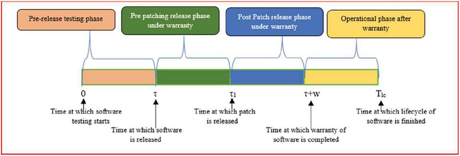
Figure 1 Lifecycle of software.
Testing cost: Testing cost refers to the complete cost of testing the software till it is released by the testing team. As development of numerous test cases and their implementation is required, this necessitates the efforts. Let us suppose c is the testing cost per unit testing effort. Hence, the testing cost associated with testing effort is denoted by and is represented as follows:
| (4) |
Market Opportunity Cost: The cost incurred due to the delayed entry of software into the market is known as market opportunity cost. This cost escalates with the delay in software release. We adopted the quadratic form of market opportunity cost as proposed by Jiang, Sarkar, and Jacob (2012). The market opportunity cost is denoted by and is expressed as follows:
| (5) |
Phase 1 (Pre-release testing phase): In this phase, the testing team identifies and reports faults to the development team. The total number of faults detected during this period is determined by aggregating the reported faults from the testing team and is given as follows:
| (6) |
The cost of detecting faults during this phase is calculated as follows:
| (7) |
Where is the rate at which software faults are detected in the interval .
Phase 2 (Pre patching release phase under warranty) : During this phase, referred to as the pre-patch-release phase, the development team addresses the unfixed bugs reported by users by developing patches. The patch is released at the end of this phase to fix the bugs. At time patch is released and is the time where patch is developed. The total number of faults detected during this interval is calculated as follows:
| (8) |
Where is the number of faults remained in the pre-release testing process and is the fault detection/removal rate in the interval . The cost incurred during this phase is calculated as follows:
| (9) |
Phase3 (Post Patch release phase under warranty) : During this interval, users may encounter failures due to bugs that were not addressed in previous phases. Consequently, these bugs are reported by users to the development team for further debugging processes. It is assumed that by the end of the warranty period, a patch will be released to address the remaining faults. The total number of faults detected or removed during this interval is calculated accordingly.
| (10) |
Where is the number of faults remained in the first and second phase and is the fault removal rate in the interval .
The cost incurred during this phase is calculated as follows:
| (11) |
Phase 4 (Operational phase after warranty) : In the post-warranty phase, any faults detected during this period are addressed after the warranty period has expired. The total number of faults identified during this phase is determined as follows:
| (12) |
Where is the number of faults remained in the first, second phase and third phase. is the fault removal rate in the interval .
The cost incurred during this phase is calculated as follows:
| (13) |
It should be noted that no patches are released to users over the last interval , as once the support cycle i.e., is completed, management will release a new version of the software. The total cost incurred is obtained by the combination of cost associated in every phase and is given below:
5 Numerical Illustration
To demonstrate the applicability of model, we have considered fault removal rate is represented by an exponential distribution. We have considered distinct fault detection rates for users and testers. The fault detection rate for testers is denoted as b, while for users, it is represented as . The mean value function of the SRGM is expressed as follows:
| (15) |
The Weibull distribution is utilized to define the effort function W(t) as follows:
| (16) |
Table 3 Data set (Obha (1984))
| Test Time | Cumulative Execution | Cumulative |
| (Weeks) | Time (CPU Hours) | Faults |
| 1 | 2.45 | 15 |
| 2 | 4.90 | 44 |
| 3 | 6.86 | 66 |
| 4 | 7.84 | 103 |
| 5 | 9.52 | 105 |
| 6 | 12.89 | 110 |
| 7 | 17.10 | 146 |
| 8 | 20.47 | 175 |
| 9 | 21.43 | 179 |
| 10 | 23.35 | 206 |
| 11 | 26.23 | 233 |
| 12 | 27.67 | 255 |
| 13 | 30.93 | 276 |
| 14 | 34.77 | 298 |
| 15 | 38.61 | 304 |
| 16 | 40.91 | 311 |
| 17 | 42.67 | 320 |
| 18 | 44.66 | 325 |
| 19 | 47.65 | 328 |
Further, we have estimated the model parameters of the effort function and mean value function using the dataset described in Table 3. The data set has 328 fault content that took 19 weeks and 47 hours of CPU time to fix. The fault detection rate is assumed to be equal in each phase i.e., bb and testing effort function is also assumed to have equal rate in each phase i.e., W(t)W(t). We have used SPSS 20.0 to estimate of parameters. The obtained results are: total testing effort consumed , shape parameter (k) 1.144967, scale parameter (v) 0.003546, fault detection rate (b) 0.013328, total number of faults (a) 571, software lifecycle T. This indicates that initially software has 571 number of faults and the fault detection rate to detect or remove the fault by a tester is 0.013328. Next, we’ll delve into the cumulative number of faults detected or removed in every phase, considering our assumptions, along with the associated costs in each phase.
The detected/removed faults in the phase is given by
| (17) |
Using Equation (7) for the cost associated in the phase to detect/remove the faults is
| (18) |
During the interval , the cumulative number of faults detected is given by
| (19) |
Using Equation (9) for the cost associated in the phase to detect the faults is described below:
The detected/removed faults in the phase is
| (20) |
The cost associated in the phase can be calculated by using Equation (11) and is described below:
| (21) |
The detected/removed faults in the phase is
| (22) |
The cost associated in the phase can be calculated by using Equation (13) and is given by:
| (23) |
The total cost is calculated by summing all the costs associated with each phase, including testing costs and market opportunity costs. Thus, the total cost is
| (24) |
5.1 Genetic Algorithm
In this section, Genetic Algorithm (GA) is used to optimize software release time and patch release times, minimizing overall costs given in Equation (5). GA is an efficient heuristic search and optimization technique. It gives the best result as compared to other metaheuristics problem-solving technique while considering large-scale problems. It is employed when traditional optimization approaches have difficulty in determining the optimal solution to a given problem. This algorithm is based on random searches Goldberg (1989). Kapur et al. (2009) optimized the cost function software testing by using genetic algorithm. Hsu and Huang (2014) proposed three weighted combinations i.e., weighted geometric, weighted harmonic combinations, and weighted arithmetic and investigated the application of weighted assignments to GA with several effective operators. Kim, Lee and Baik (2015) proposed an efficient technique for estimation of the parameters of SRGM by employing real-valued genetic algorithm. For the allocation of effort between detection and correction in the testing phase, Kumar et al. (2017) introduced an optimal control model and utilized GA to optimize detection and correction efforts. In their study (Kumar et al., 2019), they developed a decision model for defining warranty and pricing policies for a new product, employing GA to determine optimal values throughout the product’s lifecycle. The GA process involves generation, evaluation, and creation of an initial population of chromosomes selected randomly. After that, the fitness of the newly generated chromosomes is assessed. The following sub-processes are used to produce new chromosomes in the main process:
(1) Selection: Two parent chromosomes are selected.
(2) Crossover: Offspring are produced by crossing the parent chromosomes and have a crossover probability.
(3) Mutation: The offspring have distinct loci of mutation, and there is also a certain probability of mutation.
(4) Accepting: The population is expanded by including the new offspring.
(5) Replace: The next iteration is uses the next addition (if necessary)
(6) Test: As soon as the satisfactory result is given in the end condition, the process gets stopped and the optimal value is returned as an output.
(7) Loop: To find more solutions, the process is restarted.
The fitness function for cost minimization is outlined below, and Table 4 provides the parameters used in the Genetic algorithm.
| (25) |
| Parameters | Values |
| Population size | 50 |
| Selection tournament size | 2 |
| Reproduction crossover fraction | 0.8 |
| Crossover ratio | 1 |
| Migration fraction | 0.2 |
| Migration interval | 20 |
| Stopping criteria generations | 25 |
| Stopping stall generations | 100 |
Initially, we need to define the values of cost parameter before the optimization of above equation. We have used Genetic algorithm in MATLAB to get the optimal values. Let us assume the fault detection ratio r, r, r for the intervals , and respectively. Also we have assumed, the testing cost per unit time c, market opportunity cost c, the cost associated with testing team for detection/removal of faults before releasing software c, the cost associated with user for removal of faults after releasing software and before releasing patch c, the cost associated with user for removal of faults after releasing patch in the warranty period c, and the cost associated with user for removal of faults after warranty period c. Let us consider the software company has given the warranty i.e. (number of weeks). We have used the assumed values of cost parameters in Equation (5) and optimized by Genetic algorithm in MATLAB to find the optimal values of software release time and patch release time. The optimal result obtained for software release time weeks, software release time weeks and the total cost of software 3091.564. We have used the values mentioned above to summarise the phase-wise faults in Table 5 discovered by the tester and user. Out of 571 number of faults, 405 number of faults were removed by testing team before the release of software i.e. pre-release phase . Among, the remaining number of faults, 127 number of faults are removed in the before patching post release phase . Among, the remaining number of faults of faults, 24 faults are removed in the post patch release phase under warranty and 13 faults are removed in the post warranty phase .
Table 5 Phase wise description of removed faults
| Phase | Mean Value Function | Number of Faults Removed |
| Pre release phase | 405 | |
| Before patching post release phase | 126.907 (127 approx.) | |
| Post patch release phase under warranty | 24 | |
| Post warranty phase | 13 |
Table 6 Impact on cost and release time with the variation in r
| Software Release | Patch Release | ||||
| r | r | r | Time () | Time () | Cost |
| 0.21 | 0.3 | 0.4 | 20.489 | 24.004 | 3094.387 |
| 0.22 | 0.3 | 0.4 | 20.594 | 24.031 | 3093.567 |
| 0.23 | 0.3 | 0.4 | 20.689 | 24.303 | 3093.117 |
| 0.24 | 0.3 | 0.4 | 20.859 | 24.444 | 3092.276 |
| 0.25 | 0.3 | 0.4 | 20.983 | 24.5 | 3091.659 |
| 0.26 | 0.3 | 0.4 | 21.356 | 24.55 | 3090.747 |
| 0.27 | 0.3 | 0.4 | 21.507 | 24.553 | 3090.469 |
| 0.28 | 0.3 | 0.4 | 21.52 | 24.57 | 3090.279 |
| 0.29 | 0.3 | 0.4 | 21.55 | 24.58 | 3090.093 |
Table 7 Impact on cost and release time with the variation in r
| Software Release | Patch Release | ||||
| r | r | r | Time () | Time () | Cost |
| 0.2 | 0.31 | 0.4 | 20.05 | 23.028 | 3094.247 |
| 0.2 | 0.32 | 0.4 | 20.387 | 23.094 | 3089.698 |
| 0.2 | 0.33 | 0.4 | 20.746 | 24 | 3087.111 |
| 0.2 | 0.34 | 0.4 | 20.812 | 24.1 | 3085.006 |
| 0.2 | 0.35 | 0.4 | 21.13 | 24.212 | 3082.334 |
| 0.2 | 0.36 | 0.4 | 21.29 | 24.544 | 3080.771 |
| 0.2 | 0.37 | 0.4 | 21.401 | 24.753 | 3079.237 |
| 0.2 | 0.38 | 0.4 | 21.73 | 24.9 | 3077.929 |
| 0.2 | 0.39 | 0.4 | 22 | 25 | 3077.029 |
Table 8 Impact on cost and release time with the variation in r
| Software Release | Patch Release | ||||
| r | r | r | Time () | Time () | Cost |
| 0.2 | 0.3 | 0.41 | 21.764 | 24.009 | 3104.445 |
| 0.2 | 0.3 | 0.42 | 21.94 | 24.1 | 3117.376 |
| 0.2 | 0.3 | 0.43 | 22.081 | 24.1 | 3129.748 |
| 0.2 | 0.3 | 0.44 | 22.212 | 24.2 | 3141.855 |
| 0.2 | 0.3 | 0.45 | 22.346 | 24.231 | 3153.464 |
| 0.2 | 0.3 | 0.46 | 22.469 | 24.49 | 3165.08 |
| 0.2 | 0.3 | 0.47 | 22.58 | 24.51 | 3175.946 |
| 0.2 | 0.3 | 0.48 | 22.704 | 24.62 | 3186.629 |
| 0.2 | 0.3 | 0.49 | 22.815 | 24.71 | 3196.952 |
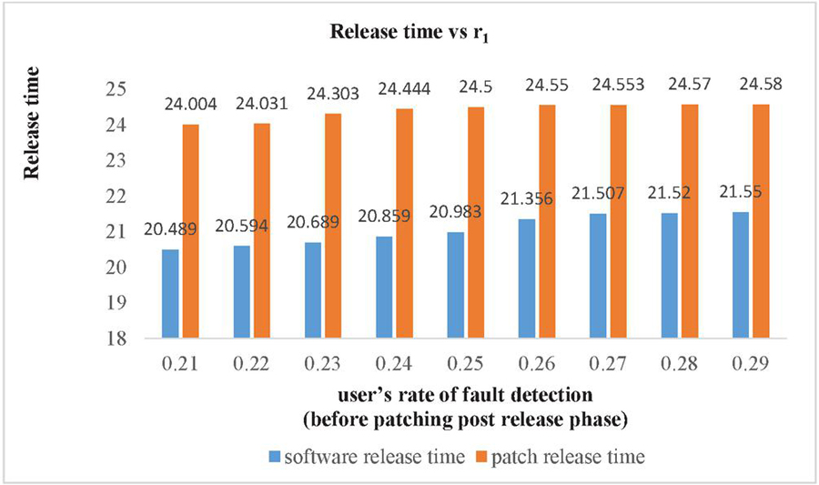
Figure 2 Impact on Software release time and patch release time of user’s fault detection rate after the release of Software.
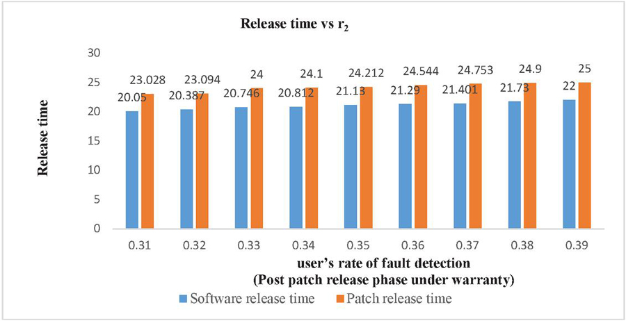
Figure 3 Impact on Software release time and patch release time of user’s fault detection rate after the release of patch.
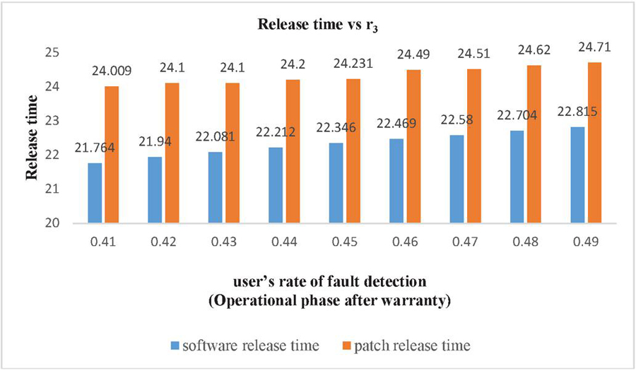
Figure 4 Impact on Software release time and patch release time of user’s fault detection rate in operational phase.

Figure 5 Impact on software’s total cost of user’s fault detection rate after the release of Software.
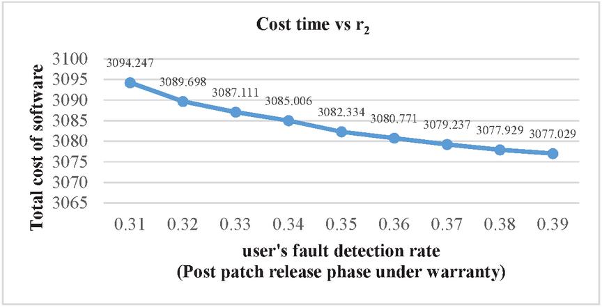
Figure 6 Impact on software’s total cost of user’s fault detection rate after the release of patch.
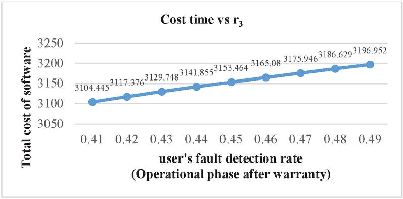
Figure 7 Impact on software’s total cost of user’s fault detection rate in operational phase.
6 Sensitivity Analysis
Sensitivity analysis is a measurement of determining how the objective function varies as the variable’s values change. The findings examine the impact of deviation in the values of variables on the software system that are varied under consideration and analyses the variable with the maximum impact on the system. The impact of change in parameters is evaluated and observed on testing cost, software release time and patch release time. We have used total number of faults (a) 571 and fault detection rate (b) 0.013328 in every case as estimated by SPSS 20.0 based on the above-mentioned dataset. We have used the same values of cost parameters for optimization of parameters and varied the values of r, r and r to perform the analysis. Consequently, Table 6 represents impact on cost and release time by varying the values of r in increasing order. It shows that with the increase in the value of r (i.e. user’s rate of fault detection in the interval ) while keeping the values of r (i.e. user’s rate of fault detection in the interval ) and r fixed (i.e. user’s rate of fault detection in the interval ), there is decrease in total testing cost with the increase in the software release time and patch release time. Similarly, the impact on cost and release time with the variation in r is shown in Table 7. In Table 7, we have fixed the values of r and r and varied the values of r in the increasing order which gave the expected result as there is decrease in the total testing cost and the increase in the software release time and patch release time. Whereas there is slightly different result obtained while varying the values of r and keeping the values of r and r fixed. Further, the impact on cost and release time with the variation in r is shown in Table 8. The result in Table 8 shows that there is increase in the release time as well as in the total cost. This is practically possible as, r is the user’s rate of fault detection in the interval . This is the post warranty period and a phase prior to the end of the lifecycle of a software product. In this phase after which software companies do not provide any assistance to remove any bug or fault. As it is considered a better option to release an updated version of software in place of removing the faults or bugs in the phase where a software is about to complete its life cycle. Since, a software is in its last phase of lifecycle may have more number of bugs or faults which will need a testing to remove them and hence testing cost will increase. The impact of change in the value of r, r and r on release times are shown in the Figures 2–4. While the impact of variation of r, r and r on the testing cost is shown in Figures 5–7.
7 Conclusion
Some of the most essential areas of policymaking in the software industries are decisions about the release and testing of software product. Generally, software industries release their product after investing a large amount of time in testing the software to attain the reliability of software so that there is reduction in the risk of software failure. However, a delay in software release leads in a loss of market opportunity cost. Now days, software firms release their product early to achieve a large market share and removes the faults by releasing patches. In this research, we address critical decision-making areas in the software industry concerning software release and testing. Traditionally, software firms invest significant time in testing to ensure reliability, aiming to mitigate the risk of software failure. However, delaying software release entails a loss in market opportunity. Today, many firms opt for early release strategies to capture a larger market share and address faults through subsequent patches. Our study develops a testing effort-based cost model within a warranty framework, considering four key phases of the software lifecycle: pre-release testing , pre-patch release , post-patch release under warranty , and operational phases . We utilize exponential distribution for modeling and employ Genetic Algorithm optimization to determine optimal software release and patch times, resulting in values of 20.278 weeks and 23.064 weeks, respectively. Across the phases, our model identifies and removes varying numbers of faults: 405 faults in pre-release testing, 127 faults in pre-patch release, 24 faults in post-patch release, and 13 faults in the post-warranty phase. While our research focuses on single patching, our model can be extended to accommodate multiple patches in the future. Additionally, future improvements may involve integrating budget and reliability considerations into the optimization process, as well as incorporating fuzzy logic and error generation for enhanced realism and accuracy.
References
Anand, A., M. Agarwal, Y. Tamura, and S. Yamada. (2017). Economic impact of software patching and optimal release scheduling. Quality and Reliability Engineering International 33(1):149–157. doi: \nolinkurl10.1002/qre.1997.
Anand, A., J. Kaur, and S. Inoue. 2020. Reliability modeling of multi-version software system incorporating the impact of infected patching. International Journal of Quality & Reliability Management 37(6/7): 1071–1085. doi: \nolinkurl10.1108/IJQRM-07-2019-0247.
Aggrawal, D., J. Kaur, and A. Anand. 2022. Modeling software patching process inculcating the impact of vulnerabilities discovered and disclosed. In System Assurances 143–153. doi: \nolinkurl10.1016/B978-0-323-90240-3.00009-6.
Bibyan, R., and S. Anand. 2022. Ranking of Multi-release Software Reliability Growth Model Using Weighted Distance-Based Approach. In Optimization Models in Software Reliability 355–373. doi: \nolinkurl10.1007/978-3-030-78919-0_16.
Dhavakumar, P., and N. P. Gopalan 2021. An efficient parameter optimization of software reliability growth model by using chaotic grey wolf optimization algorithm. Journal of Ambient Intelligence and Humanized Computing 12(2):3177–3188. doi: \nolinkurl10.1007/s12652-020-02476-z.
Goel, A. L., and K. Okumoto. 1979. Time-dependent error-detection rate model for software reliability and other performance measures. IEEE transactions on Reliability 28(3):206–211. doi: \nolinkurl10.1109/TR.1979.5220566.
Golberg, D. E. 1989. Genetic algorithms in search, optimization, and machine learning. Addion Wesley.
Hossain, S. A., and R. C. Dahiya. 1993. Estimating the parameters of a non-homogeneous Poisson-process model for software reliability. IEEE Transactions on Reliability 42(4):604–612. doi: \nolinkurl10.1109/24.273589.
Hsu, C. J., and C.Y. Huang. 2014. Optimal weighted combinational models for software reliability estimation and analysis. IEEE Transactions on Reliability 63(3):731–749. doi: \nolinkurl10.1109/TR.2014.2315966.
Huang, Y. S., K. C. Chiu, and W. M. Chen. 2022. A software reliability growth model for imperfect debugging. Journal of Systems and Software 188:111267. doi: \nolinkurl10.1016/j.jss.2022.111267.
Jiang, Z., and Sarkar. S. 2003. Optimal software release time with patching considered. In Workshop on Information Technologies and Systems. Seattle, WA, USA.
Jiang, Z., S. Sarkar, and V.S. Jacob. 2012. Postrelease testing and software release policy for enterprise-level systems. Information Systems Research 23(3-part-1): 635–657. doi: \nolinkurl10.2307/23276478.
Kaur, J., A. Anand, O. Singh, and V. Kumar 2021. Measuring software reliability under the influence of an infected patch. Yugoslav Journal of Operations Research 31(2):249–264. doi: \nolinkurl10.2298/YJOR200117005K.
Kapur, P. K., D.N. Goswami, A. Bardhan, and O. Singh. 2008. Flexible software reliability growth model with testing effort dependent learning process. Applied Mathematical Modelling 32(7):1298–1307. doi: \nolinkurl10.1016/j.apm.2007.04.002.
Kapur, P. K., A.G. Aggarwal, K. Kapoor, and G. Kaur. 2009. Optimal testing resource allocation for modular software considering cost, testing effort and reliability using genetic algorithm. International Journal of Reliability, Quality and Safety Engineering 16(06):495–508. doi: \nolinkurl10.1142/S0218539309003538.
Kapur, P. K., S. Panwar, O. Singh, and V. Kumar. 2019. Joint release and testing stop time policy with testing-effort and change point. In Risk based technologies 209–222. doi: \nolinkurl10.1007/978-981-13-5796-1_12.
Kansal, Y., G. Singh, U. Kumar, and P. K. Kapur. 2016. Optimal release and patching time of software with warranty. International Journal of System Assurance Engineering and Management 7(4):462–468. doi: \nolinkurl10.1007/s13198-016-0510-7.
Kim, T., K. Lee, and J. Baik. 2015. An effective approach to estimating the parameters of software reliability growth models using a real-valued genetic algorithm. Journal of Systems and Software 102:134–144. doi: \nolinkurl10.1016/j.jss.2015.01.001.
Kumar, V., P. Mathur, R. Sahni, and M. Anand 2016. Two-dimensional multi-release software reliability modeling for fault detection and fault correction processes. International Journal of Reliability, Quality and Safety Engineering 23(03):1640002. doi: \nolinkurl10.1142/S0218539316400027.
Kumar, V., R. Sahni, and A. K. Shrivastava. 2016. Two-dimensional multi-release software modelling with testing effort, time and two types of imperfect debugging. International Journal of Reliability and Safety 10(4):368–388. doi: \nolinkurl10.1504/IJRS.2016.10005347.
Kumar, V., P.K. Kapur, N. Taneja, and R. Sahni. 2017. On allocation of resources during testing phase incorporating flexible software reliability growth model with testing effort under dynamic environment. International Journal of Operational Research 30(4):523–539. doi: \nolinkurl10.1504/IJOR.2017.087829.
Kumar, V., V. B. Singh, A. Dhamija, and S. Srivastav. 2018. Cost-reliability-optimal release time of software with patching considered. International Journal of Reliability, Quality and Safety Engineering 25(04):1850018. doi: \nolinkurl10.1142/S0218539318500183.
Kumar, V., V.B. Singh, A. Garg, and G. Kumar. 2018. Selection of optimal software reliability growth models: a fuzzy DEA ranking approach. In Quality, IT and business operations 347–357. doi: \nolinkurl10.1007/978-981-10-5577-5_28.
Kumar, V., P.K. Kapur, R. Sahni, and A.K. Shrivastava. 2018. Testing time and effort-based successive release modeling of a software in the presence of imperfect debugging. In Quality, IT and Business Operations 421–434. doi: \nolinkurl10.1007/978-981-10-5577-5_33.
Kumar, V., B. Sarkar, A.N. Sharma, and M. Mittal. 2019. New product launching with pricing, free replacement, rework, and warranty policies via genetic algorithmic approach. International Journal of Computational Intelligence Systems 12(2):519. doi: \nolinkurl10.2991/ijcis.d.190401.001.
Kumar, V., P. Saxena, and H. Garg. 2021. Selection of optimal software reliability growth models using an integrated entropy–Technique for Order Preference by Similarity to an Ideal Solution (TOPSIS) approach. Mathematical Methods in the Applied Sciences doi: \nolinkurl10.1002/mma.7445.
Lee, D. H., I. H. Chang, and H. Pham. 2020. Software reliability model with dependent failures and SPRT. Mathematics 8(8):1366. doi: \nolinkurl10.3390/math8081366.
Li, X., M. Xie, and S.H. Ng. 2010. Sensitivity analysis of release time of software reliability models incorporating testing effort with multiple change-points. Applied Mathematical Modelling 34(11):3560–3570. doi: \nolinkurl10.1016/j.apm.2010.03.006.
Li, Q., and H. Pham. 2021. Software Reliability Modeling Incorporating Fault Detection and Fault Correction Processes with Testing Coverage and Fault Amount Dependency. Mathematics 10(1):60. doi: \nolinkurl10.3390/math10010060.
Lin, C. T., and C.Y. Huang. 2008. Enhancing and measuring the predictive capabilities of testing-effort dependent software reliability models. Journal of Systems and Software 81(6):1025–1038. doi: \nolinkurl10.1016/j.jss.2007.10.002.
Narang, S., P.K. Kapur, D. Damodaran, and A.K Shrivastava 2018. Bi-criterion problem to determine optimal vulnerability discovery and patching time. International Journal of Reliability, Quality and Safety Engineering 25(01):1850002. doi: \nolinkurl10.1142/S021853931850002X.
Ohba, M. 1984. Inflection S-shaped software reliability growth model. In Stochastic models in reliability theory Springer 144–162. doi: \nolinkurl10.1109/TR.1984.5221826.
Peng, R., Y.F. Li, W.J. Zhang, and Q.P. Hu. 2014. Testing effort dependent software reliability model for imperfect debugging process considering both detection and correction. Reliability Engineering & System Safety 126:37–43. doi: \nolinkurl10.1016/j.ress.2014.01.004.
Pham, H., and X. Zhang 1997. An NHPP software reliability model and its comparison. International Journal of Reliability, Quality and Safety Engineering 4(03):269–282. doi: \nolinkurl10.1142/S0218539397000199.
Pham, H. 2014. A new software reliability model with Vtub-shaped fault-detection rate and the uncertainty of operating environments. Optimization 63(10):1481–1490. doi: \nolinkurl10.1080/02331934.2013.854787.
Saxena, P., V. Kumar, and M. Ram, 2021. Ranking of Software Reliability Growth Models: A Entropy-ELECTRE Hybrid Approach. Reliability: Theory & Applications SI 2 (64):95–113.
Saxena, P., N. Singh, A.K. Shrivastava, and V. Kumar. 2021. Testing effort based SRGM and release decision under fuzzy environment. International Journal of Reliability and Safety 15(3):123–140. doi: \nolinkurl10.1504/IJRS.2021.123275.
Saxena, P., V. Kumar, and M. Ram. 2022. A novel CRITIC-TOPSIS approach for optimal selection of software reliability growth model (SRGM). Quality and Reliability Engineering International 38(5):2501–2520. doi: \nolinkurl10.1002/qre.3087.
Tian, Q., C. W. Yeh, and C. C. Fang. 2022. Bayesian Decision Making of an Imperfect Debugging Software Reliability Growth Model with Consideration of Debuggers’ Learning and Negligence Factors. Mathematics 10(10):1689. doi: \nolinkurl10.3390/math10101689.
Tickoo, A., P. K. Kapur, A. K. Shrivastava, and S. K. Khatri. 2016. Testing effort based modeling to determine optimal release and patching time of software. International Journal of System Assurance Engineering and Management 7(4):427–434. doi: \nolinkurl10.1007/s13198-016-0470-y.
Tickoo, A., P.K. Kapur, A.K. Shrivastava, and S.K. Khatri. 2018. Discrete-time framework for determining optimal software release and patching time. In Quality, IT and Business Operations 129–141. doi: \nolinkurl10.1007/978-981-10-5577-5_11.
Yamada, S., M. Ohba, and S. Osaki. 1983. S-shaped reliability growth modeling for software error detection. IEEE Transactions on reliability 32(5):475–484. doi: \nolinkurl10.1109/TR.1983.5221735.
Yamada, S., K. Tokuno, and S. Osaki. 1992. Imperfect debugging models with fault introduction rate for software reliability assessment. International Journal of Systems Science 23(12):2241–2252. doi: \nolinkurl10.1080/00207729208949452.
Zhang, C., Y. Yuan, W. Jiang, Z. Sun, Y. Ding, M. Fan, L. Wenyu, W. Yafei, S. Wen, and K. Liu. 2021. Software Reliability Model Related to Total Number of Faults Under Imperfect Debugging. In International Conference on Intelligent Automation and Soft Computing Springer, 48–60. doi: \nolinkurl10.1007/978-3-030-81007-8_7.
Biographies

Palak Saxena is a promising young researcher serving as a Research Scholar at the Department of Mathematics within the Amity Institute of Applied Sciences at Amity University Uttar Pradesh, Noida, India. She received her MSc degree in Mathematics from Kumaun University, India and PhD from Amity Institute of Applied Sciences, Amity University, Noida, India. Her research interest includes software reliability and mathematical modelling. She has published several research papers in the area of software reliability in international journals and conferences. Palak possesses a strong command over various software tools and programming languages, including SPSS, and MATLAB. Her expertise and dedication make her a valuable asset in his field of study.

Vijay Kumar received his MSc in Applied Mathematics and MPhil in Mathematics from Indian Institute of Technology (IIT), Roorkee, India in 1998 and 2000, respectively. He has completed his PhD from the Department of Operational Research, University of Delhi. Currently, he is a Professor in the Department of Mathematics, Amity Institute of Applied Sciences, Amity University, Noida, India. He is co-editor of two book and has published more than 70 research papers in the areas of software reliability, mathematical modelling and optimisation in international journals and conferences of high repute. His current research interests include software reliability growth modelling, optimal control theory and marketing models in the context of innovation diffusion theory. He has edited special issues of IJAMS and RIO journal. He is an editorial board member of IJSA, Springer. He is a life member of Society for Reliability Engineering, Quality and Operations Management (SREQOM).

Stuti Tandon is working as an Assistant Professor in School of Computer Applications at Manav Rachna International Institute of Research and Studies, India. Stuti received her MCA degree from VTU, Belgaum; India. MBA degree from Symbiosis University. She did her PhD in Information Technology from Amity University – Noida, India. She has published a number of papers in preferred Journals and chapters in books, and participated in a range of forums on software engineering. She also presented various academic as well as research-based papers at several national and international conferences. Her research activity is set to explore the developmental role for the software industry.

Kuldeep Chaudhary is an accomplished academic professional serving as an Assistant Professor at the Department of Mathematics, Amity Institute of Applied Sciences, Amity University Uttar Pradesh, Noida, India. With an impressive teaching and research career spanning his expertise lies in various research domains, including Mathematical modeling, optimization, software reliability, and Fuzzy theory, among others. He has published more than 30 research articles in the International Journals/book chapters/conferences.

Mangey Ram received the Ph.D. degree major in Mathematics and minor in Computer Science from G. B. Pant University of Agriculture and Technology, Pantnagar, India in 2008. He has been the Faculty Member for around 15 years and has taught several core courses in pure and applied mathematics at undergraduate, postgraduate, and doctorate levels. He is currently the Research Professor & Dean (Research Collaborations) at Graphic Era Deemed to be University, Dehradun, India. Before joining the Graphic Era University, he was the Deputy Manager (Probationary Officer) with Syndicate Bank for a short period.
Prof. Ram is Editor-in-Chief of International Journal of Mathematical, Engineering and Management Sciences; Journal of Reliability and Statistical Studies; Journal of Graphic Era University; Series Editor of six Book Series with Elsevier, CRC Press-A Taylor and Frances Group, Walter De Gruyter Publisher Germany, River Publishers, and the Guest Editor & Associate Editor with various journals. He has published 400 plus publications (journal articles/books/book chapters/conference articles) in IEEE, Taylor & Francis, Springer Nature, Elsevier, Emerald, World Scientific and many other national and international journals and conferences. Also, he has published more than 60 books (authored/edited) with international publishers like Elsevier, Springer Nature, CRC Press-A Taylor and Frances Group, Walter De Gruyter Publisher Germany, River Publisher. His fields of research are reliability theory and applied mathematics. Dr. Ram is a Senior Member of the IEEE, Senior Life Member of Operational Research Society of India, Society for Reliability Engineering, Quality and Operations Management in India, Indian Society of Industrial and Applied Mathematics, He has been a member of the organizing committee of several international and national conferences, seminars, and workshops.
He has been conferred with “Young Scientist Award” by the Uttarakhand State Council for Science and Technology, Dehradun, in 2009. He has been awarded the “Best Faculty Award” in 2011; “Research Excellence Award” in 2015; “Outstanding Researcher Award” in 2018 for his significant contribution in academics and research at Graphic Era Deemed to be University, Dehradun, India. Recently, he has been received the “Excellence in Research of the Year-2021 Award” by the Honourable Chief Minister of Uttarakhand State, India & “Emerging Mathematician of Uttarakhand-2022” award by the Director, Directorate of Higher Education Uttarakhand at Uttarakhand Open University, Haldwani, India.
Journal of Reliability and Statistical Studies, Vol. 17, Issue 1 (2024), 77–108.
doi: 10.13052/jrss0974-8024.1714
© 2024 River Publishers