A Study on One-Parameter Entropy-Transformed Exponential Distribution and Its Application

Mathew Stephen^1,*, David Ikwuoche John² and Yaska Mutah³

¹Department of Mathematics, Statistics and Computer Science, Kwararafa University Wukari, Wukari Nigeria
²Department of Mathematics and Statistics, Federal University Wukari, 200, Katsina-Ala Road, Wukari, Wukari, Nigeria
³Department of Mathematics and Statistics, The Federal Polytechnic Mubi, Adamawa State
E-mail: matsteve231@gmail.com
*Corresponding Author

Received 23 November 2023; Accepted 12 April 2024

Abstract

This study presents the Entropy-Transformed Exponential Distribution (EnTrED), in an attempt to enhancing the flexibility and applicability of the traditional exponential distribution. The study explores the statistical properties of the EnTrED, including mode, quantile function, reliability, moments, and hazard function. The parameters of the distribution were estimated using maximum likelihood estimation, and the stability of these estimates was thoroughly evaluated through extensive Monte Carlo simulation. The simulation results demonstrated that the maximum likelihood estimates of the model parameters were well-behaved. Additionally, Empirical assessments against alternative distributions underscores the robustness of the EnTrED as a superior model for analyzing life data.

Keywords: Entropy-transformed exponential distribution (EnTrED), memoryless property, hazard rate, survival analysis, reliability analysis, time-dependent hazard.

1 Introduction

Modeling real life data is integral in many areas of applied studies such as life sciences, biochemistry, geosciences, cosmology, statistical mechanics, social sciences, linguistics, biology, information technology, and even science fiction films. Considerable efforts have been done to construct new distributions for survival data. However, there still remain many problems involving real data, which are not contemplated by existing probability models (Percontini, Gomes-Silva, da Silva and Handique, 2021). Suppose a random variable c follow an exponential distribution and its probability density function (P.D.F) and cumulative distribution function (C.D.F) are given by;

$$f(c)=\phi e^{-\phi c}\text{and}F(c)=1-e^{-\phi c},\text{for all}c\ge 0\text{and}\phi >0$$

(1)

For this model, the probability of an event occurring is most likely independent of time i.e.,$P(C>c+dc/C>c)=P(C>dc)=e^{-\phi dc}$ which implies the memoryless property. This property may not hold in some practical scenarios. Also, for this model In (1), when dealing with systems that wear out or age over time, the exponential distribution may not accurately capture the increasing failure rate since $h(c)=\phi$ (Nelsen, 1987). In addressing the above challenges to make the exponential distribution more flexible and applicable to a wide range of real-life scenarios, several researches have proposed different transformation techniques. (Owoloko, Oguntunde and Adejumo, 2015) studied the “transmuted exponential distribution”, (El-Damrawy, Teamah and El-Shiekh, 2022) derived the “Truncated bivariate Kumaraswamy exponential distribution”, (Chesneau, Kumar, Khetan and Arshad, 2022) derived the “modified weighted exponential distribution”, (Ozkan and Golbasi, 2023) proposed the “Generalized Marshall-Olkin exponentiated exponential distribution” amongst others.

Dragan and Isaic-Maniu (2019) described the pseudo-entropic transformation also called entropy transformation by (Aziz, Husain, and Ahmed, 2021) which has some unique features. The transformation can be summarized with the expression in (2) (for more details see (Aziz, Husain, and Ahmed, 2021)).

$$f(c)=\frac{d}{dx}[R(c)]\log [R(c)]$$

(2)

where $R(c)$ is the survival function of a baseline probability distribution.

By incorporating both the rate of change of the reliability function and the logarithm of the reliability, which can be related to the hazard function, a more flexible exponential model that allow for time-varying hazard rates with memory effects can be created. This can lead to a more realistic and flexible exponential model for reliability analysis and survival data, especially when modeling systems or processes where the failure rate is not constant over time.

The aim of this research is to propose a novel distribution called the entropy transformed exponential distribution, to derive some of its properties, estimate its parameter using the method of maximum likelihood, validate through simulation the stability of the model and to demonstrate its applicability using real life data sets. The rest of this article is organized into sections as follows; In Section 2 the entropy transformed exponential distribution (EnTrED) is formally introduced, the statistical and reliability properties of the EnTrED and the maximum likelihood estimate (MLE) of the parameter of the parameter is derived and presented. In Section 3, the stability of the EnTrED was determined through a simulation study and the application of the EnTrED in modelling real-life data sets and the study concludes in Section 4.

2 Entropy Transformed Exponential Distribution

2.1 Exponential Distribution

The probability density function (PDF) and cumulative density function (CDF) of the exponential distribution is given by (1). By definition, the survival function is given by the equation

$$R(c)=1-F(c)=1-(1-e^{-\phi c})=e^{-\phi c};\exists c>0\text{and}\phi >0$$

(3)

2.1.1 Entropy transform exponential distribution

According to (Dragan and Isaic-Maniu, 2019), if a random variable c has an exponential distribution, then the random variable will have an entropy transformed (or the pseudo-entropic) exponential distribution if its PDF satisfies the equation;

$$f_{\mathit{new}}(c)={\int }_0^{\mathrm{\infty }}{R}^{\prime }(c)\log (R(c))\mathit{d}c=1$$

(4)

The survival function of the exponential distribution is given by;

$$R^{\prime }(c)=\frac{d}{dc}(e^{-\phi c})=-\phi e^{-\phi c}$$

and substituting the log of the survival function and its derivative into Equation (4) yields the following:

$$f_{\mathit{new}}(c)=-\phi e^{-\phi c}\log (e^{-\phi c})=-\phi e^{-\phi c}(-\phi c)={\phi }^{2}c{e}^{-\phi c}$$
$$f_{\mathit{new}}(c)={\phi }^{2}c{e}^{-\phi c}$$	(5)

$\exists c>0$ and $\phi >0$.

To validate the that (5) satisfies the condition in (4), it has to be shown that the integral over the range of (5) is unity.

$$f_{\mathit{new}}(c)={\int }_0^{\mathrm{\infty }}{\phi }^{2}c{e}^{-\phi c}\mathit{d}c=1$$

(6)

By using integration by parts, let

$$u=c;dc=e^{-\phi c}\Rightarrow c=\int e^{-\phi c}\mathit{d}c=-\frac{e^{-\phi c}}{\phi }.$$

(7)

On substituting into (6), and simplifying, it can easily be shown that

$$-\frac{c{e}^{-\phi c}}{\phi }-\int -\frac{e^{-\phi c}}{\phi }dc={(-\frac{c{e}^{-\phi c}}{\phi }+\frac{e^{-\phi c}}{{\phi }^2}]}_0^{\mathrm{\infty }}=1$$

satisfying the condition in (4) and validating the $f_{\mathit{new}}(c)$ model.

Definition 1: a random variable c is said to have an entropy transformed exponential distribution if it satisfies (5) $\exists c>0$ and $\phi >0$.

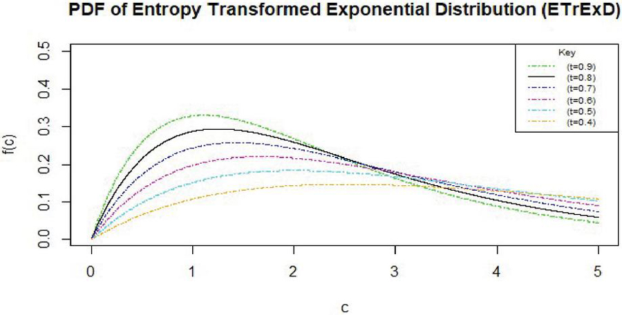
Figure 1 Plot (where $t=\phi$).

Figure 1 displays the of the EnTrED, revealing a right-skewed distribution.

By the fundamental theory of calculus the $\mathrm{Pr}(C\underset{¯}{<}c)$ represents the CDF of the random variable and can be obtained by solving the following;

$$F_{\mathit{new}}(c)={\int }_0^c{f}_{\mathit{new}}(c)\mathit{d}c$$

(8)

As it has been shown,

$$\int f_{\mathit{new}}(c)dc=-\frac{c{e}^{-\phi c}}{\phi }-\int -\frac{e^{-\phi c}}{\phi }dc=(-\frac{c{e}^{-\phi c}}{\phi }+\frac{e^{-\phi c}}{{\phi }^2}]$$

(9)

Since the definition the CDF is a function, whose output yields the $\mathrm{Pr}(C\le c)$, evaluating (9) will yield the CDF of $E_n{T}_{r}ED$. Thus,

$$F_{\mathit{new}}(c)=e^{-\phi c}(e^{-\phi c}-1-\phi c).$$

(10)

Definition 2: for a random variable c, the expression in equation (10) defines the CDF of the Entropy Transformed Exponential Distribution $(E_n{T}_{r}ED)$, $\exists c>0$ and $\phi >0$.

The CDF of the distribution is displayed in Figure 2, satisfying the condition that all $c>0$ and $\phi >0$.

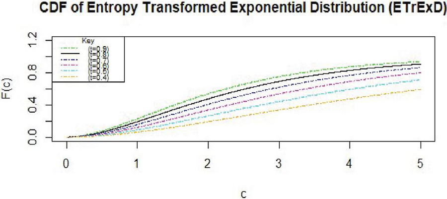
Figure 2 CDF plot (where $t=\phi$).

2.1.2 Asymptotic behaviour

The asymptotic behavior of the PDF provides insights into the tails or extreme values of the distribution. The limit of EnTrED as $c\to [0,\mathrm{\infty }]$ is 0.

$\underset{y\to [0]}{lim}[{\phi }^{2}c{e}^{-\phi c}]$	$={\phi }^{2}0e^{-\phi \mathrm{\hspace{0.17em}0}}=0\mathit{\hspace{1em}}\text{and}$
$\underset{y\to [\mathrm{\infty }]}{lim}[{\phi }^{2}c{e}^{-\phi c}]$	$={\phi }^2\mathrm{\infty }{e}^{-\phi \mathrm{\infty }}=\mathrm{\infty }{e}^{-\mathrm{\infty }}=0$	(11)

The limit of EnTrED in the tails is 0. This indicates that the probability of observing values in those tails is infinitesimally in the regions. This is consistent with the condition that the total probability over the entire range of possible values for a random variable is unity.

2.1.3 Properties of EnTrED

Quantile function (Q(C))

The EnTrED has the ability to generate random variates or random samples that follow the distribution’s characteristics since its quantile function can be expressed in terms of the Lambert W ($W(\cdot )$) function (Further details on the $W(\cdot )$ can be found in Corless et al. 1996).

Theorem 1: Let c be a random variable distributed with EnTrED. Then for every fixed $\phi >0$, and $0>k>1$, the quantile function is given as follows;

$$q_c=\frac{\log \left(\frac{W(k)e^{-1}-1}{k}\right)}{2\phi }$$

(12)

Proof To obtain the quantile function, the CDF of the random variable c must be inverted.

$$q_c=F_{\mathit{new}}^{-1}(c)$$
$$F_{\mathit{new}}(c)=e^{-\phi c}(e^{-\phi c}-1-\phi c)$$
$$k=e^{-\phi c}(e^{-\phi c}-1-\phi c)$$
$$k{e}^{\phi c}=e^{-\phi c}-1-\phi c;\Rightarrow k{e}^{\phi c}-e^{-\phi c}=-1-\phi c$$
$$e^{-\phi c}-k{e}^{\phi c}=1+\phi c;\Rightarrow e^{-\phi c}(1-k{e}^{-1})=1+\phi c$$
$$(1-k{e}^{2\phi c})=\frac{1+\phi c}{e^{-\phi c}};\Rightarrow (1-k{e}^{2\phi c})=e^{\phi c}(1+\phi c)$$	(13)

Let $h=1+\phi c$; $\Rightarrow c=\frac{h-1}{\phi }$, then, on substitution into (13), we have that

$1-k{e}^{2\phi c}$	$=e^{\phi \left(\frac{h-1}{\phi }\right)}\left(1+\phi \left({\displaystyle \frac{h-1}{\phi }}\right)\right)$
	$=e^{\phi \left(\frac{h-1}{\phi }\right)}\left(1+\phi \left({\displaystyle \frac{h-1}{\phi }}\right)\right)=h{e}^h{e}^{-1}$	(14)

Using Lambert’s function, $W{e}^w=W$, Equation (2.1.3) can be written as

$$1-k{e}^{2\phi c}=W(k)e^{-1}$$

$$k{e}^{2\phi c}=W(k)e^{-1}+1$$

$$2\phi c=\log \left(\frac{W(k)e^{-1}+1}{k}\right)$$

$$c=\frac{\log \left(\frac{W(k)e^{-1}+1}{k}\right)}{2\phi }$$

Therefore,

$$q_c=\frac{\log \left(\frac{W(k)e^{-1}+1}{k}\right)}{2\phi }$$

(15)

Which ends the proof.

The graphical plot for the quantile function is presented in Figure 3.

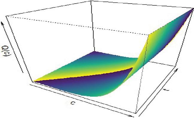
Figure 3 Quantile function plot (where $t=\phi$).

Raw moments

For a random variable c, the raw moment is a quantitative measure that characterizes various aspects of its probability distribution. The moment function of the random variable is used to study many important properties of distribution such as dispersion, tendency, skewness and kurtosis.

Theorem 2: Let a random variable $c\sim EnTrED(\phi )$, then, the raw moment is given by the equation;

$$r^{th}={\left(\frac{1}{\phi }\right)}^r\mathrm{\Gamma }(r+2)$$

(16)

Proof

For any continuous random variable with a valid PDF $f(c)$, the $r^{th}$ moment ${\mathrm{\Xi }}_r$ is given by:

$r^{th}$	$=E[c^r]={\displaystyle {\int }_0^{\mathrm{\infty }}}{c}^r{f}_{\mathit{new}}(c)\mathit{d}c$
$r^{th}$	$={\displaystyle {\int }_0^{\mathrm{\infty }}}{c}^r{\phi }^{2}c{e}^{-\phi c}\mathit{d}c;r^{th}={\displaystyle {\int }_0^{\mathrm{\infty }}}{c}^{r+1}{\phi }^2{e}^{-\phi c}\mathit{d}c$	(17)

By transformation, let

$$b=\phi c;c=\frac{b}{\phi };\frac{db}{dc}=\phi ;\Rightarrow dc=\frac{1}{\phi }db$$

On substituting into Equation (2.1), the following is obtained;

$r^{th}$	$={\displaystyle {\int }_0^{\mathrm{\infty }}}{\left({\displaystyle \frac{b}{\phi }}\right)}^{r+1}{\phi }^2{e}^{-b}{\displaystyle \frac{1}{\phi }}\mathit{d}b$
$r^{th}$	$={\left({\displaystyle \frac{1}{\phi }}\right)}^{r+1-1}{\displaystyle {\int }_0^{\mathrm{\infty }}}{(b)}^{r+1}{e}^{-b}\mathit{d}b.$	(18)

Since gamma of z is expressed as $\mathrm{\Gamma }(z)={\int }_0^{\mathrm{\infty }}{x}^{z-1}{e}^{-x}\mathit{d}x$, Equation (2.1) can be transformed into

$$r^{th}={\left(\frac{1}{\phi }\right)}^r\mathrm{\Gamma }(r+2)$$

(19)

Therefore, the $r^{th}$ of a random variable c with entropy transformed exponential distribution is expressed as shown in Equation (19), which completes the proof.

Probability weighted moments

Probability Weighted Moments $(P_M^W)$ are expressed as expectations of functions of a random variable, premise on the condition that the ordinary moments of the random variable exist. For a random variable C the probability weighted moments is defined by the expression;

$$P_M^W={\int }_0^{\mathrm{\infty }}{c}^r{F}_{\mathit{new}}^s(c)f_{\mathit{new}}(c)\mathit{d}c$$

(20)

Theorem 3: Let a random variable $c\sim EnTrED(\phi )$, then, the $(P_M^W)$ of EnTrED is given by;

$$P_M^W=\varphi \mathrm{\Gamma }(r+2+k)$$

(21)

Proof

To obtain the $P_M^W$ for EnTrED, we make the substitution of Equation (6) for $f_{\mathit{new}}(c)$ and (10) for $F_{\mathit{new}}(c)$ into (20). Thus;

$P_M^W$	$={\displaystyle {\int }_0^{\mathrm{\infty }}}{c}^r{(e^{-\phi c}(e^{-\phi c}-1-\phi c))}^s({\phi }^{2}c{e}^{-\phi c})\mathit{d}c$	(22)
$P_M^W$	$={\displaystyle {\int }_0^{\mathrm{\infty }}}{\phi }^2{c}^{r+1}{(e^{-\phi c}-1-\phi c)}^s{e}^{-\phi c(s+1)}\mathit{d}c$
$P_M^W$	$={\displaystyle {\int }_0^{\mathrm{\infty }}}{\phi }^2{c}^{r+1}{(e^{-\phi c}-A)}^s{e}^{-\phi c(s+1)}\mathit{d}c$	(23)

Where; $A=1-\phi c$

${(a+b)}^n$	$={\displaystyle \sum _{i=0}^{\mathrm{\infty }}}\left({\displaystyle \genfrac{}{}{0pt}{}{n}{k}}\right)(a^{n-k}{b}^k);{(1-y)}^{b-1}$
	$={\displaystyle \sum _{i=0}^{\mathrm{\infty }}}{b}_i{y}^i;b_i={(-1)}^i\left({\displaystyle \genfrac{}{}{0pt}{}{b-1}{i}}\right)$	(24)

Using the Binomial sum of a series presented in Equation (2.1), it can be shown that

$${(e^{-\phi c}-A)}^s=\sum _{j=0}^{\mathrm{\infty }}\left(\genfrac{}{}{0pt}{}{s}{j}\right){(-1)}^j{A}^j{e}^{-\phi c(n-j)}$$

(25)

Thus,

$P_M^W$	$={\displaystyle {\int }_0^{\mathrm{\infty }}}{\phi }^2{c}^{r+1}{\displaystyle \sum _{j=0}^s}\left({\displaystyle \genfrac{}{}{0pt}{}{s}{j}}\right){(-1)}^j{A}^j{e}^{-\phi c(n-j)}{e}^{-\phi c(s+1)}dc$	(26)
$P_M^W$	$={\displaystyle {\int }_0^{\mathrm{\infty }}}{\phi }^2{c}^{r+1}{\displaystyle \sum _{j=0}^s}\left({\displaystyle \genfrac{}{}{0pt}{}{s}{j}}\right){(-1)}^j{(1-\phi c)}^j{e}^{-\phi c(n-j)}{e}^{-\phi c(s+1)}dc$	(27)

Also, by expanding using Binomial sum of a series in (2.1), it can be shown that,

$${(1-\phi c)}^j=\sum _{k=0}^{\mathrm{\infty }}{(-1)}^j\left(\genfrac{}{}{0pt}{}{j}{k}\right){(\phi c)}^k$$

(28)

Substitute (28) into (27). Then we have that;

$P_M^W$	$={\displaystyle {\int }_0^{\mathrm{\infty }}}{\phi }^2{c}^{r+1}{\displaystyle \sum _{j=0}^s}\left({\displaystyle \genfrac{}{}{0pt}{}{s}{j}}\right){(-1)}^j{\displaystyle \sum _{k=0}^{\mathrm{\infty }}}{(-1)}^k$
	$\mathrm{\hspace{1em}}\times \left({\displaystyle \genfrac{}{}{0pt}{}{j}{k}}\right){(\phi c)}^k{e}^{-\phi c(n-j)}{e}^{-\phi c(s+1)}dc$
$P_M^W$	$={\displaystyle {\int }_0^{\mathrm{\infty }}}\mathrm{\Theta }{\phi }^{2+k}{c}^{r+1+k}{e}^{-\phi c(n-j)}{e}^{-\phi c(s+1)}\mathit{d}c$

Where;

$\mathrm{\Theta }$	$={\displaystyle \sum _{j=0}^s}\left({\displaystyle \genfrac{}{}{0pt}{}{s}{j}}\right){(-1)}^{j+k}{\displaystyle \sum _{k=0}^{\mathrm{\infty }}}\left({\displaystyle \genfrac{}{}{0pt}{}{j}{k}}\right)$
$P_M^W$	$={\displaystyle {\int }_0^{\mathrm{\infty }}}\mathrm{\Theta }{\phi }^{2+k}{c}^{r+1+k}{e}^{-\phi c(n-j)-\phi c(s+1)}\mathit{d}c$	(29)
$P_M^W$	$=\mathrm{\Theta }{\phi }^{2+k}{\displaystyle {\int }_0^{\mathrm{\infty }}}{c}^{r+1+k}{e}^{-\phi c(n-j-s-1)}\mathit{d}c$	(30)

By transformation, let;

$$u=\phi c(n-j-s-1);c=\frac{u}{\phi (n-j-s-1)};\frac{du}{dc}=\phi (n-j-s-1);$$
$$dc=\frac{du}{\phi (n-j-s-1)}$$	(31)

Substitute (31) into (30).

$P_M^W$	$=\mathrm{\Theta }{\phi }^{2+k}{\displaystyle {\int }_0^{\mathrm{\infty }}}{\left({\displaystyle \frac{u}{\phi (n-j-s-1)}}\right)}^{r+1+k}{e}^{-u}{\displaystyle \frac{du}{\phi (n-j-s-1)}}$
$P_M^W$	$=\mathrm{\Theta }{\phi }^{2+k}{\left({\displaystyle \frac{1}{\phi (n-j-s-1)}}\right)}^{r+1+k}$
	$\mathrm{\hspace{1em}}\times {\displaystyle {\int }_0^{\mathrm{\infty }}}{u}^{r+1+k}{e}^{-u}{\displaystyle \frac{du}{\phi (n-j-s-1)}}$	(33)
$P_M^W$	$=\mathrm{\Theta }{\phi }^{2+k}{(\phi (n-j-s-1))}^{-(r+2+k)}{\displaystyle {\int }_0^{\mathrm{\infty }}}{u}^{r+1+k}{e}^{-u}\mathit{d}u$	(34)
$P_M^W$	$=\mathrm{\Theta }{\phi }^{2+k}{(\phi (n-j-s-1))}^{-(r+2+k)}{\displaystyle {\int }_0^{\mathrm{\infty }}}{u}^{r+1+k}{e}^{-u}\mathit{d}u$	(35)
$P_M^W$	$=\mathrm{\Theta }{\phi }^{2+k}{(\phi (n-j-s-1))}^{-(r+2+k)}{\displaystyle {\int }_0^{\mathrm{\infty }}}{u}^{(r+2+k)-1}{e}^{-u}\mathit{d}u$	(36)
$P_M^W$	$=\varphi \mathrm{\Gamma }(r+2+k)$	(37)

Where; $\varphi =\mathrm{\Theta }{\phi }^{2+k}{(\phi (n-j-s-1))}^{-(r+2+k)}$

Conditional moment

A useful tool for understanding the distributional properties of random variables is the conditional moments $(M_q)$. Assume that C is a random variable, or an event, such that $X=C>c$, then the expected value of $C^r$ given the condition $X$ is represented by the conditional moment of order $r$, which is written as $E[C^r/X]$. For the random variable $c$ with EnTrED, the conditional moment is derived by;

$$M_q=\frac{[\phi t^{r+1}{e}^{-\phi t}-e^{-\phi t}]}{S(c)}$$

(38)

Proof

The conditional moment of a random variable with continuous distribution is given by;

$$M_q=E[C^r/X]=\frac{1}{S(c)}{\int }_t^{\mathrm{\infty }}{c}^r{f}_{\mathit{new}}(c)\mathit{d}c$$

(39)

For $c\sim EnTrED(\phi )$, make the substitution of Equation (6) for the PDF of the EnTrED in Equation (39).

$M_q$	$=E[C^r/X]={\displaystyle \frac{1}{S(c)}}{\displaystyle {\int }_t^{\mathrm{\infty }}}{c}^r{\phi }^{2}c{e}^{-\phi c}\mathit{d}c$
$M_q$	$=E[C^r/C>c]={\displaystyle \frac{{\phi }^2}{S(c)}}{\displaystyle {\int }_t^{\mathrm{\infty }}}{c}^{r+1}{e}^{-\phi c}dc$

By using integration by parts, let

$$u=c;dc=e^{-\phi c}\Rightarrow c=\int e^{-\phi c}\mathit{d}c=-\frac{e^{-\phi c}}{\phi }.$$

This implies that

$M_q$	$={\displaystyle \frac{{\phi }^2}{S(c)}}\left(-{\displaystyle \frac{c^{r+1}{e}^{-\phi c}}{\phi }}-{\displaystyle \int }-{\displaystyle \frac{e^{-\phi c}}{\phi }}dc\right)$
	$={\displaystyle \frac{1}{S(c)}}{(-\phi c^{r+1}{e}^{-\phi c}+e^{-\phi c}]}_t^{\mathrm{\infty }}$
$M_q$	$={\displaystyle \frac{1}{S(c)}}{(-\phi c^{r+1}{e}^{-\phi c}+e^{-\phi c}]}_t^{\mathrm{\infty }}$
	$={\displaystyle \frac{1}{S(c)}}[-\phi \cdot {\mathrm{\infty }}^{r+1}{e}^{-\phi \cdot \mathrm{\infty }}+e^{-\phi \cdot \mathrm{\infty }}+\phi t^{r+1}{e}^{-\phi t}-e^{-\phi t}]$
$M_q$	$={\displaystyle \frac{[\phi t^{r+1}{e}^{-\phi t}-e^{-\phi t}]}{S(c)}}$	(40)

Where $S(c)$ is the survival function of EnTrED (as defined in Equation (48)), thus completing the proof.

Mean

Theorem 4: The mean of a random variable $c\sim EnTrED(\phi )$ is expressed as follows.

$$r^1={\left(\frac{1}{\phi }\right)}^1\mathrm{\Gamma }(1+2)=\left(\frac{1}{\phi }\right)\mathrm{\Gamma }(3)$$

(41)

Proof

The mean of a random variable c with EnTrED can be obtained as the first moment. This can be derived by substituting unity into the ${\mathrm{\Xi }}_r$ moment in (19).

$$r^1={\left(\frac{1}{\phi }\right)}^1\mathrm{\Gamma }(1+2)=\left(\frac{1}{\phi }\right)\mathrm{\Gamma }(3)$$

(42)

Which completes the proof.

Harmonic mean (Har.M)

Theorem 5: the harmonic mean of a random variable $c\sim EnTrED(\phi )$ is expressed as follows.

$$Har.M=\frac{1}{c}{\int }_0^{\mathrm{\infty }}{\phi }^2{e}^{-\phi c}\mathit{d}c=-{\frac{1}{c}\phi c{e}^{-\phi c}|}_0^{\mathrm{\infty }}=\phi$$

(43)

Proof

The harmonic mean of a random variable c with $E_n{T}_{r}ED$ can be obtained by solving the expression given below.

$Har.M$	$=E\left[{\displaystyle \frac{1}{c}}\right]={\displaystyle {\int }_0^{\mathrm{\infty }}}{\displaystyle \frac{1}{c}}{f}_{\mathit{new}}(c)\mathit{d}c$	(44)
$Har.M$	$={\displaystyle {\int }_0^{\mathrm{\infty }}}{\displaystyle \frac{1}{c}}{\phi }^{2}c{e}^{-\phi c}\mathit{d}c$
$Har.M$	$={\displaystyle \frac{1}{c}}{\displaystyle {\int }_0^{\mathrm{\infty }}}{\phi }^2{e}^{-\phi c}\mathit{d}c=-{{\displaystyle \frac{1}{c}}\phi c{e}^{-\phi c}|}_0^{\mathrm{\infty }}=\phi$	(45)

Which ends the proof.

Mode (Md)

Theorem 6: the mode of a random variable $c\sim EnTrED(\phi )$ is defined as follows.

$$Md=\frac{1}{\phi }$$

(46)

Proof

The mode of a random variable

$$\frac{d}{dc}(\log (f_{\mathit{new}}(c)))=0$$
$$\frac{d}{dc}(\log ({\phi }^{2}c{e}^{-\phi c}))=0$$
$$\frac{d}{dc}(\log ({\phi }^{2}c)-\phi c)=0$$
$$\frac{1}{c}-\phi =0;\Rightarrow c=\frac{1}{\phi }$$
$$Md=\frac{1}{\phi }$$	(47)

Which ends the proof.

Survival function (S(c))

Survival function can be defined as the probability that an event happened after time, $t$. It models time to-an-event and takes note of the time it takes for an event to occur. Given the CDF of a probability function, the survival function is the probability of survival beyond time $c$ and is defined by;

$$S(c)=1-F_{\mathit{new}}(c)=1-e^{-\phi c}(e^{-\phi c}-1-\phi c)$$

(48)

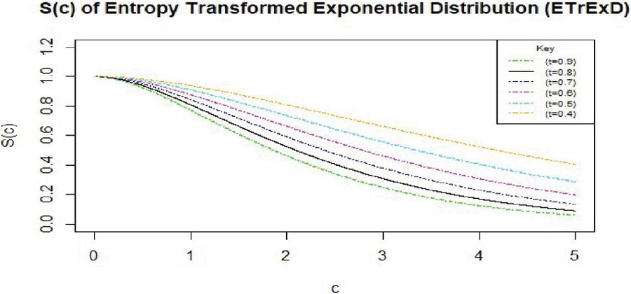
Figure 4 Survival function plot (where $t=\phi$).

The survival function of the EnTrED is presented in Figure 4. This depicts the probability that an event has not occurred by time ($c$). The function is characterized by a gradual decrease from $1-0$ as $c$ increases, thus, signifying a diminishing likelihood of no event occurrence over time. Ultimately, as $c$ increases, the survival function value approaches 0, suggesting that the event is almost certain to occur after a sufficiently long time.

Hazzard function (H(c))

The hazard function is also known as the failure rate is defined as the conditional probability of failure of an item/device given that the item has survived to the time, t. The hazard rate function of a random variable $c$ is the ratio of the PDF, $f_{\mathit{new}}(c)$ to the survival function, and is given by:

$$H(c)=\frac{f_{\mathit{new}}(c)}{S_{\mathit{new}}(c)}=\frac{{\phi }^{2}c{e}^{-\phi c}}{1-e^{-\phi c}(e^{-\phi c}-1-\phi c)}$$

(49)

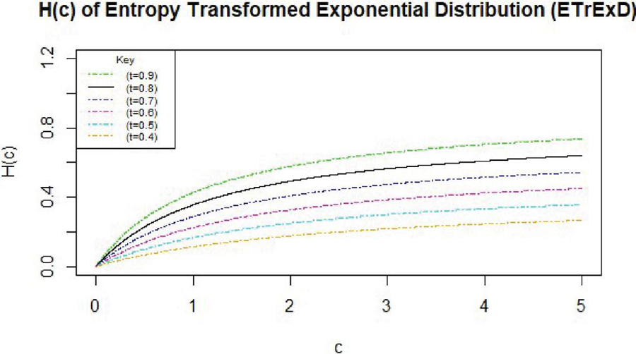
Figure 5 Hazzard function plot (where $t=\phi$).

The hazard function provided represents the instantaneous risk of event occurrence for model EnTrED as a function of $c$ with $\phi$ as a parameter. As shown in Figure 5, the function increases gradually with c, showing a linear-like behavior. However, as $c$ increases, the hazard function reaches a peak and becomes asymptotically constant. The behavior is influenced by the parameter $\phi$, where higher values result in steeper increases in the hazard rate.

Characteristic function

This characteristics function is useful and has some properties which gives it a genuine role in mathematical statistics. It is used for generating moments, characterization of distributions and in analysis of linear combination of independent random variables.

Theorem 6: the characteristic function of a random variable $c\sim EnTrED(\phi )$ is defined by the following equation.

$Q_c(t)$	$={\displaystyle \sum _{i=0}^n}{\displaystyle \frac{{(-1)}^n{(t)}^{2n}}{2n!}}\left({\left({\displaystyle \frac{1}{\phi }}\right)}^{(2n)}\mathrm{\Gamma }(2n+2)\right)$
	$\mathrm{\hspace{1em}}+i{\displaystyle \sum _{i=0}^n}{\displaystyle \frac{{(-1)}^n{(t)}^{2n+1}}{(2n+1)!}}\left({\left({\displaystyle \frac{1}{\phi }}\right)}^{(2n+1)}\mathrm{\Gamma }(2n+3)\right)$	(50)

Proof

The characteristics function of a random variable $c$ is given by;

$$Q_c(t)=E[e^{itc}]={\int }_0^{\mathrm{\infty }}{e}^{itc}{f}_{\mathit{new}}(c)\mathit{d}c$$

(51)

Expressing $e^{itc}$ in trigonometric form, we have that

$$e^{itc}=\cos (tc)+i\sin (tc)$$
$$E[e^{itc}]=E[\cos (tc)+i\sin (tc)]$$
$$E[e^{itc}]=E[\cos (tc)]+E[i\sin (tc)]$$	(52)

Using the power series expansion, it can be shown that

$\sin (tc)$	$={\displaystyle \sum _{i=0}^n}{\displaystyle \frac{{(-1)}^n{(tc)}^{2n+1}}{\left(2n+1\right)!}}\mathit{\hspace{1em}}\text{and}$
$\cos (tc)$	$={\displaystyle \sum _{i=0}^n}{\displaystyle \frac{{(-1)}^n{(tc)}^{2n}}{2n!}}$	(53)

This implies that

$E[e^{itc}]$	$=E\left[{\displaystyle \sum _{i=0}^n}{\displaystyle \frac{{(-1)}^n{(tc)}^{2n}}{2n!}}+i{\displaystyle \sum _{i=0}^n}{\displaystyle \frac{{(-1)}^n{(tc)}^{2n+1}}{(2n+1)!}}\right]$
	$={\displaystyle \sum _{i=0}^n}{\displaystyle \frac{{(-1)}^n{(t)}^{2n}}{2n!}}E[c^{2n}]+i{\displaystyle \sum _{i=0}^n}{\displaystyle \frac{{(-1)}^n{(t)}^{2n+1}}{(2n+1)!}}E[c^{(2n+1)}]$
$Q_c(t)$	$={\displaystyle \sum _{i=0}^n}{\displaystyle \frac{{(-1)}^n{(t)}^{2n}}{2n!}}{r}^{2n}+i{\displaystyle \sum _{i=0}^n}{\displaystyle \frac{{(-1)}^n{(t)}^{2n+1}}{(2n+1)!}}{r}^{(2n+1)}$	(54)

Where $r^{(2n)}$ and $r^{(2n+1)}$ are the moments of the random variable $c$ for $r=2n$ and $r=2n+1$ respectively.

As obtained in Equation (19), $E[c^r]=r^{th}={(\frac{1}{\phi })}^r\mathrm{\Gamma }(r+2)$.

It follows that

$r^{(2n)}$	$={\left({\displaystyle \frac{1}{\phi }}\right)}^{(2n)}\mathrm{\Gamma }(2n+2)={\left({\displaystyle \frac{1}{\phi }}\right)}^{(2n)}\mathrm{\Gamma }(2n+2)$
$r^{(2n+1)}$	$={\left({\displaystyle \frac{1}{\phi }}\right)}^{(2n+1)}\mathrm{\Gamma }(2n+1+2)={\left({\displaystyle \frac{1}{\phi }}\right)}^{(2n+1)}\mathrm{\Gamma }(2n+3)$
$Q_c(t)$	$={\displaystyle \sum _{i=0}^n}{\displaystyle \frac{{(-1)}^n{(t)}^{2n}}{2n!}}\left({\left({\displaystyle \frac{1}{\phi }}\right)}^{(2n)}\mathrm{\Gamma }(2n+2)\right)$
	$\mathrm{\hspace{1em}}+i{\displaystyle \sum _{i=0}^n}{\displaystyle \frac{{(-1)}^n{(t)}^{2n+1}}{(2n+1)!}}\left({\left({\displaystyle \frac{1}{\phi }}\right)}^{(2n+1)}\mathrm{\Gamma }(2n+3)\right)$	(55)

Thus, completing the proof.

Order statistic

Order statistics are essential for describing the distribution and behavior of random variables because they provide the sorted values of observations taken from a sample. Given a random sample of size $k$, the order statistics are denoted as $X_{(1)},X_{(2)},\mathrm{\dots },X_{(k)}$, where $X_{(1)}$ represents the smallest observation, $X_{(2)}$ the second smallest, to $X_{(k)}$, which denotes the largest observation. The $k^{th}$ order statistic of a random variable is given as;

$f_{(k,n)}(c)={\displaystyle \frac{n!}{(k-1)!(n-k)!}}{f}_{\mathit{new}}(c){[F_{\mathit{new}}(c)]}^{k-1}{[1-F_{\mathit{new}}(c)]}^{n-k}$

Expanding ${[1-F_{\mathit{new}}(c)]}^{n-k}$ using the Binomial theorem, we have

$${[1-F_{\mathit{new}}(c)]}^{n-k}=\sum _{p=0}^{\mathrm{\infty }}\left(\genfrac{}{}{0pt}{}{n-k}{p}\right){(-1)}^p{[F_{\mathit{new}}(c)]}^p$$

(57)

Therefore, equation (57) becomes;

$$f_{(k,n)}(c)=\sum _{p=0}^{\mathrm{\infty }}\left(\genfrac{}{}{0pt}{}{n-k}{p}\right)\frac{n!}{(k-1)!(n-k)!}{(-1)}^p{f}_{\mathit{new}}(c){[F_{\mathit{new}}(c)]}^{p+k-1}$$

(58)

Theorem 8: The $k^{th}$ order statistic of a random variable with EnTrED is given by;

$$f_{(k,n)}(c)=\omega ({\phi }^{2}c{e}^{-\phi c}){[e^{-\phi c}(e^{-\phi c}-1-\phi c)]}^{p+k-1}$$

(59)

Proof

To obtain the $k^{th}$ order statistic of the EnTrED, we make the substitution (6) for $f_{\mathit{new}}(c)$ and (10) for $F_{\mathit{new}}(c)$ in Equation (58). Therefore,

$f_{(k,n)}(c)$	$={\displaystyle \sum _{p=0}^{\mathrm{\infty }}}\left({\displaystyle \genfrac{}{}{0pt}{}{n-k}{p}}\right){\displaystyle \frac{n!}{(k-1)!(n-k)!}}{(-1)}^p({\phi }^{2}c{e}^{-\phi c})$
	$\mathrm{\hspace{1em}}\times {[e^{-\phi c}(e^{-\phi c}-1-\phi c)]}^{p+k-1}$	(60)
$f_{(k,n)}(c)$	$=\omega ({\phi }^{2}c{e}^{-\phi c}){[e^{-\phi c}(e^{-\phi c}-1-\phi c)]}^{p+k-1}$	(61)

Where;

$$\omega =\sum _{p=0}^{\mathrm{\infty }}\left(\genfrac{}{}{0pt}{}{n-k}{p}\right)\frac{n!{(-1)}^p}{(k-1)!(n-k)!}.$$

Information measures

In information theory, information measures are numbers that are used to quantify different characteristics of information, uncertainty, and entropy. These metrics have been applied in a variety of domains, such as statistics, machine learning, communication theory, and cryptography, where it is essential to comprehend and quantify uncertainty and information. This subsection will develop the Renyi entropy and associated Arimoto measure for the EnTrED.

1. Renyi entropy

The Rényi entropy measures bear the name of the mathematician Alfréd Rényi. It generalizes the concept of Shannon entropy, providing a parameterized family of entropy measures. This can be defined as follows;

$$E_R(k)=\frac{1}{1-k}\log {\int }_0^{\mathrm{\infty }}{f}_{\mathit{new}}^k(c)\mathit{d}c;\mathrm{for}k>1,k\ne 1$$

(62)

Suppose a random variable $c\sim EnTrED(\phi )$, then the degree of uncertainty can be obtained by substituting (6) for $f_{\mathit{new}}(c)$ in equation in Equation (62) as follows;

$E_R(k)$	$={\displaystyle \frac{1}{1-k}}\log {\displaystyle {\int }_0^{\mathrm{\infty }}}{({\phi }^{2}c{e}^{-\phi c})}^k\mathit{d}c$	(63)
$E_R(k)$	$={\displaystyle \frac{1}{1-k}}\log \left[{\phi }^{2k}{\displaystyle {\int }_0^{\mathrm{\infty }}}{c}^k{e}^{-\phi ck}\mathit{d}c\right]$	(64)

From (16), ${\int }_0^{\mathrm{\infty }}{c}^k{e}^{-\phi ck}\mathit{d}c$ is equivalent to the moment of the density function. Thus, on substituting into (64), we obtain the following;

$$E_R(k)=\frac{\log [{\phi }^{2k}{r}^{th}]}{1-k}$$

(65)

2. Arimoto measure of entropy

A means of comparing the uncertainty or disorder in probability distributions is the Arimoto measure of entropy, which is often referred to as the “information divergence entropy” or the “information radius entropy.” The following formula defines this:

$A_K(c)$	$={\displaystyle \frac{k}{1-k}}\left[{(E_k(\theta ))}^{\frac{1}{k}}-1\right]$
	$={\displaystyle \frac{k}{1-k}}\left({\displaystyle {\int }_0^{\mathrm{\infty }}}{(f_{\mathit{new}}^k(c)dc)}^{\frac{1}{k}}-1\right);\mathrm{for}k>1,k\ne 1$	(66)

If $c\sim EnTrED(\phi )$, then on substituting (6) into (66), the Arimoto measure of entropy is derived as follows;

$A_K(c)$	$={\displaystyle \frac{k}{1-k}}\left({\left({\displaystyle {\int }_0^{\mathrm{\infty }}}{\phi }^{2}c{e}^{-\phi c}\mathit{d}c\right)}^{\frac{1}{k}}-1\right)$	(67)
$A_K(c)$	$={\displaystyle \frac{k}{1-k}}\left(\left({\phi }^{\frac{2}{k}}{\displaystyle {\int }_0^{\mathrm{\infty }}}{c}^{\frac{1}{k}}{e}^{-\frac{\phi c}{k}}\mathit{d}c\right)-1\right)$	(68)

On substituting the transformation in (7) into (68), we have that,

$$A_K(c)=\frac{k}{1-k}\left(\left({\phi }^{\frac{2}{k}-\frac{1}{k}}{\int }_0^{\mathrm{\infty }}{b}^{\frac{1}{k}}{e}^{-\frac{b}{k}}\frac{1}{\phi }\mathit{d}b\right)-1\right)$$

which can be transformed using the gamma function as;

$$A_K(c)=\frac{k}{1-k}\left(k^{\frac{1-k}{k}}{\phi }^{\frac{k+1}{k}}\mathrm{\Gamma }\left(\frac{1}{k}\right)\right)$$

(69)

Method of parameter estimation adopted

To estimate the parameter of the EnTrED, using the maximum likelihood method, let $c_1,c_2,\mathrm{\dots },c_n$ be independent identically distributed of size (n) with probability function EnTrED, then, the likelihood function $L(\varphi )$ for EnTrED is given below

$L(\varphi )$	$={\displaystyle \prod _{i=1}^n}{f}_{\mathit{new}}(c)={\displaystyle \prod _{i=1}^n}{\phi }^{2}c{e}^{-\phi c}={\phi }^{2n}{e}^{-\phi {\sum }_{i=1}^{n}c}{\displaystyle \sum _{i=1}^n}c$	(70)
$\log (L(\varphi ))$	$=\log \left({\phi }^{2n}{e}^{-\phi {\sum }_{i=1}^{n}c}{\displaystyle \sum _{i=1}^n}c\right)$
	$=2n\log (\phi )-\phi {\displaystyle \sum _{i=1}^n}c+{\displaystyle \sum _{i=1}^n}\log (c)$

The likelihood equation in (70) is partially differentiated with respect to phi and equating to zero, we have

${\displaystyle \frac{\partial (\log (L(\varphi )))}{\partial \varphi }}$	$={\displaystyle \frac{\partial (2n\log (\phi ))}{\partial \phi }}-{\displaystyle \frac{\partial (\phi {\sum }_{i=1}^{n}c)}{\partial \phi }}$
	$\mathrm{\hspace{1em}}+{\displaystyle \frac{\partial \left({\sum }_{i=1}^n\log (c)\right)}{\partial \phi }}=0$
${\displaystyle \frac{(2n)}{\phi }}-\phi {\displaystyle \sum _{i=1}^n}c$	$=0;\Rightarrow \phi =2n{\left({\displaystyle \sum _{i=1}^n}c\right)}^{-1}$

Therefore, the MLE for the parameter of $E_n{T}_{r}ED$ is given as;

$$\phi =2n{\left(\sum _{i=1}^{n}c\right)}^{-1}$$

(71)

3 Stability Analysis

3.1 Simulation

This part uses Monte-Carlo simulation to assess the stability of the EnTrED probability model’s MLE by increasing the sample size. A random sample of sizes 30, 100, 500 and 750 was generated and using the quantile function shown in Equation (10) with the parameter values fixed at 0.3, 0.4, 0.6, and 0.9. The bias (AvAB), variance (Var), standard deviation (SD), mean square error (MSE), root mean square error (RMSE) and coefficient of variation (CV) were the metrics utilized to evaluate the stability. The calculations were done using the following formula;

$$\mathbf{\text{MSE}}=\sum _{q=1}^Q{({\stackrel{⌢}{u}}_q-u)}^2/q\mathbf{\text{RMSE}}=\sqrt{\mathbf{\text{MSE}}}AvAB=\sum _{i=1}^k|b-\widehat{b}|/k-1;$$
$$Var=\sum _{i=1}^k{(b-\widehat{b})}^2/k-1;CV=⟨(b-\widehat{b})/\widehat{b}⟩\times 100\%SD=\sqrt{Var};$$	(72)

Table 1 Simulation results and measures of accuracy

Sample
Size	Parameter	MLE	Bias	Var	SD	MSE	RMSE	CoV
30	0.3	2.7808	2.4808	22.0374	4.6944	28.1918	5.3096	168.8142
100	0.3	1.9742	1.6742	15.7767	3.9720	18.5795	4.3104	201.1996
500	0.3	0.5759	0.2759	0.6880	0.8294	0.7641	0.8741	144.0315
750	0.3	0.4604	0.1604	0.0755	0.2748	0.1012	0.3182	59.6916
30	0.4	0.4331	0.0331	0.1419	0.3766	0.1429	0.3781	86.9586
100	0.4	0.5137	0.1137	0.0094	0.0971	0.0224	0.1495	18.8955
500	0.4	0.5137	0.1137	0.0021	0.0455	0.0150	0.1225	8.8559
750	0.4	0.2728	-0.1272	0.0030	0.0552	0.0192	0.1387	20.2369
30	0.8	0.6893	-0.1107	0.0008	0.0279	0.0130	0.1142	4.0525
100	0.8	0.6506	-0.1494	0.0867	0.2944	0.1090	0.3302	45.2557
500	0.8	0.7674	-0.0326	0.0181	0.1346	0.0192	0.1385	17.5453
750	0.8	0.6873	-0.1127	0.0000	0.0055	0.0127	0.1129	0.8032
30	0.9	0.6705	-0.2295	0.0006	0.0248	0.0533	0.2308	3.7032
100	0.9	0.7790	-0.1210	0.0001	0.0086	0.0147	0.1213	1.1077
500	0.9	0.7790	-0.1210	0.0000	0.0040	0.0147	0.1211	0.5191
750	0.9	0.6687	-0.2313	0.0000	0.0049	0.0535	0.2314	0.7338

A simulation was performed and the results presented in Table 1 presents the sample size, true and MLE parameter estimates for the new model. Testing the behavior of the distribution with the aid of variance, standard deviation and standard error revealed as the sample sizes increases. The observed trend in the simulation results was as anticipated: as the sample sizes grew larger and larger, the values of the adequacy metrics (variance, standard deviation, and standard error) decreasing. This trend displayed in Figure 6 aligns with expectations for a well-fitting density model. In statistical modeling, an adequate model should ideally demonstrate reduced variability and increased precision as more data becomes available for estimation.

Therefore, the decreasing values of these adequacy metrics as the sample sizes increased can be interpreted as a positive sign. This result supports the conclusion that the EnTrED model behaves as a well-behaved density function, which is indicative of its suitability for modeling real-life data sets. In essence, the simulation results, as summarized in Table 1, indicate that the EnTrED model is a statistically sound and appropriate choice for modeling data in various applications.

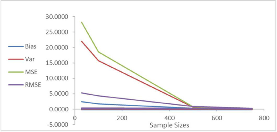
Figure 6 Measures of stability.

3.2 Empirical Application

This section uses three actual datasets to show the applicability and flexibility of the EnTrE distribution. Additionally, this part offers a comparison to other competing models and an assessment of the distribution’s goodness of fit. The models that were compared included the Sine Exponential distribution, Exponential distribution, Ram Awadh distribution and Prakaamy distribution respectively. The Kolmogrov Smirnov (KS), AIC, BIC, HQIC, and CAIC are among the adequacy metrics used. The better the model, the lower these measures’ values should be.

In this section, the empirical applicability and flexibility of the newly introduced entropy-transformed exponential distribution (EnTrED) are thoroughly examined using real-world datasets. This analysis aims to showcase the practical utility of the EnTrED model in handling diverse data scenarios. Moreover, it includes a comparative assessment of the EnTrED model against several alternative statistical distributions to assess the goodness of fit and overall performance. The datasets chosen for this evaluation are actual, real-world datasets, which adds an element of authenticity and relevance to the analysis. These datasets represent different domains or fields of study, making them suitable for assessing the versatility of the EnTrED model across various applications. To determine how well the EnTrED model performs in comparison to other statistical models, a comprehensive set of competing models is considered. These competing models include:

Table 2 Competing models

Models	PDF	Domain	Sources
Sine Exponential (SE)	$f(x;\kappa )={\displaystyle \frac{\pi }{2}}{e}^{-\kappa x}\cos \left({\displaystyle \frac{\pi }{2}}(-1e^{-\kappa x})\right)$	For $\kappa ,x>0$	(Isa, Bashiru, Ali, and Adepoju, 2022)
Exponential (E)	$f(x;\kappa )=\kappa e^{-\kappa x}$	For $\kappa ,x>0$
Ram Awadh (RA)	$f(x;\kappa )={\displaystyle \frac{{\kappa }^6}{{\kappa }^6+120}}(\kappa +x^5)e^{-\kappa x}$	For $\kappa ,x>0$	(Shukla, 2018).
Prakaamy (P)	$f(x;\kappa )={\displaystyle \frac{{\kappa }^3}{{\kappa }^3+\kappa +2}}(1+x+x^2)e^{-\kappa x}$	For $\kappa ,x>0$	(Shukla, 2018)

The first dataset was based on (Tashkandy, Nagy, Akbar, Mahmood and Gemeay, 2023) and covered the intervals between 64 successive eruptions of the Kiama Blowhole. The following is the dataset’s content: 83, 51, 87, 60, 28, 95, 8, 27, 15, 10, 18, 16, 29, 54, 91, 8, 17, 55, 10, 35, 47, 77, 36, 17, 21, 36, 18, 40, 10, 7, 34, 27, 28, 56, 8, 25, 68, 146, 89, 18, 73, 69, 9, 37, 10, 82, 29, 8, 60, 61, 61, 18, 169, 25, 8, 26, 11, 83, 11, 42, 17, 14, 9, 12

Table 3 Adequacy measures for fits using first dataset

Models	AIC	BIC	CAIC	HQIC	MLE	KS	P val	Rank
EnTrED	595.594	597.753	595.659	596.445	0.050	0.162	0.070	1
SE	599.937	602.096	600.002	600.788	0.014	0.152	0.105	2
E	601.625	603.784	601.690	602.476	0.025	0.164	0.063	3
RA	1105.328	1108.149	1105.361	1106.474	0.150	109748	2.2e-16	5
P	695.421	697.580	695.486	696.272	0.151	109743	2.2e-16	4

Table 4 95% Confidence interval estimates for first dataset

Models	MLE	SE_MLE	95% Lower CI	95% Upper CI
EnTrED	0.050	0.000	0.050	0.051
SE	0.014	0.000	0.014	0.014
E	0.025	0.000	0.025	0.025
RA	0.151	0.000	0.150	0.151
P	0.151	0.000	0.150	0.151

The second dataset, which details the number of COVID-19 cases during the first wave in Nepal in December 2020, was published by (Dhungana and Kumar, 2022). The data is shown as follows: 2, 2, 2, 2, 2, 2, 3, 2, 3, 3, 4, 2, 5, 5, 3, 2, 4, 4, 8, 4, 4, 3, 2, 3, 7, 6, 6, 11, 9, 3, 8, 7, 11, 8, 12, 12, 14, 7, 11, 12, 6, 14, 9, 9, 11, 6, 6, 5, 5, 14, 9, 15, 11, 8, 4, 7, 11, 10, 16, 2, 7, 17, 6, 8, 10, 4, 10, 7, 11, 11, 8, 7, 19, 9, 15, 12, 10, 14, 22, 9, 18, 12, 19, 21, 12, 12, 18, 8, 26, 21, 17, 13, 5, 15, 14, 11, 17, 16, 17, 23, 24, 20, 30, 18, 18, 17, 21, 18, 22, 26, 15, 13, 13, 6, 9, 17, 12, 17, 22, 7, 16, 16, 24, 28, 23, 23,19, 25, 29, 21, 9, 13, 16, 10, 17, 20, 23, 14, 12, 11, 15, 9, 18, 14, 13, 6, 16, 12, 11, 7, 3, 5, 5.

Table 5 Adequacy measures for fits using second dataset

Models	AIC	BIC	CAIC	HQIC	MLE	KS	P val	Ranks
EnTrED	1004.982	1008.012	1005.009	1006.213	0.172	0.101	0.091	1
SE	1048.172	1051.202	1048.198	1049.403	0.047	0.161	0.001	2
E	1058.388	1061.419	1058.415	1059.619	0.086	0.188	4.1e-05	3
RA	1087.025	1090.055	1087.051	1088.256	0.516	10612	2.2e-16	4
P	1087.025	1090.055	1087.051	1088.256	0.516	10595	2.2e-16	5

Table 6 95% Confidence interval estimates for second dataset

Models	Estimate	SE	95% Lower CI	95% Upper CI
EnTrED	0.172	0.001	0.170	0.174
SE	0.049	0.000	0.048	0.049
E	0.086	0.001	0.085	0.087
RA	0.517	0.003	0.510	0.523
P	0.517	0.003	0.510	0.523

The third dataset can be found in (Banerjee and Bhunia, 2022), and it details the survival periods (in days) of guinea pigs that were given various amounts of tubercle bacilli. The dataset includes the following: 12, 15, 22, 24, 24, 32, 32, 33, 34, 38, 38, 43, 44, 48, 52, 53, 54, 54, 55, 56, 57, 58, 58, 59, 60, 60, 60, 60, 61, 62, 63, 65, 65, 67, 68, 70, 70, 72, 73, 75, 76, 76, 81, 83, 84, 85, 87, 91, 95, 96, 98, 99, 109, 110, 121, 127, 129, 131, 143, 146, 146, 175, 175, 211, 233, 258, 258, 263, 297, 341, 341, 376.

Table 7 Adequacy measures for fits using third dataset

Models	AIC	BIC	CAIC	HQIC	MLE	KS	P val	Rank
EnTrED	790.567	792.843	790.624	791.473	0.020	0.134	0.153	1
SE	805.941	808.217	805.998	806.847	0.006	0.193	0.009	2
E	808.884	811.161	808.941	809.791	0.010	0.211	0.003	3
RA	856.749	859.026	856.806	857.655	0.060	59703	2.2e-16	4
P	1752.437	1754.714	1752.494	1753.343	0. 060	3.05e+11	2.2e-16	5

Table 8 95% Confidence interval estimates for third dataset

Models	Estimates	SE	95% Lower CI	95% Upper CI
EnTrED	0.0200	0.0000	0.0200	0.0201
SE	0.0057	0.0000	0.0057	0.0057
E	0.0100	0.0000	0.0100	0.0100
RA	0.0601	0.0001	0.0600	0.0602
P	0.0601	0.0001	0.0600	0.0602

As presented in Tables 3, 5 and 7, the results on the application of the EnTrED to real dataset compared to six other models revealed the applicability of the new model. It can be observed that the EnTrED has the smallest of all the information criterions (i.e., AIC, BIC, CAIC and HQIC). The profound implication of these findings is the EnTrED model’s supremacy in terms of adequacy and goodness of fit. The exceptional performance of the model is expressed in the consistently lower AIC, BIC, CAIC, and HQIC values, irrespective of dataset characteristics and shows its versatility and adaptability. This remarkable ability to capture the underlying data generation mechanisms more effectively positions the EnTrED as a formidable tool for researchers across diverse scientific areas. Its statistical flexibility and adequacy are invaluable assets in modelling complex data structures, offering researchers an advanced and dependable distribution for intricate statistical modeling and analysis tasks.

Results in Tables 4, 6 and 8 summarizes the parameter estimates along with their, standard errors and 95% confidence intervals for the models across the three data sets. The results presented provides insights into the precision of the estimates and the range within which the true parameter values are likely to fall with a specified level of confidence. As observed, the parameter estimates all fell within the 95th percent confidence interval and the difference between the upper and lower CI showed that EnTrED, SE, and E had the smallest value, thus indicating that they provide a better fit for the data sets.

4 Conclusion

In this study, ErTrED is proposed. Various statistical and reliability attributes of EnTrED, including moments, moment generating function, quantile function, hazard rate function, and mean, as well as order statistics, were examined and derived. Additionally, a rigorous simulation study was executed to assess the stability of the Maximum Likelihood Estimates (MLE) for EnTrED’s parameters, revealing their robust behavior as sample sizes increased.

To demonstrate the flexibility and adequacy of the EnTrED distribution, an empirical data analysis was carried out. The goodness of fit of the EnTrED model was scrutinized using three distinct datasets as test cases. A comparative analysis ensued, fitting the EnTrED against competing distributions, including the Sine Exponential, Exponential, Ram Awadh and Prakaamy distributions. The results of this extensive empirical data analysis pointed to the EnTrED exhibiting better fitting capabilities across the datasets. This compelling outcome underscores the potential of EnTrED as the distribution with the most adequate fit, affirming its position as a valuable tool for researchers and practitioners alike. Parameter estimation methods influences parameter estimates of a density function. In this study, we utilized the Maximum Likelihood Estimation (MLE) method. As a suggestion for future research, we recommend exploring alternative estimation methods for the EnTrED. This exploration can provide valuable insights into the robustness and accuracy of parameter estimation in diverse modeling scenarios.

References

Aziz, A., Husain, Q., and Ahmed, M. (2021). The Entropy Transformed Rayleigh Distribution: Properties and Applications. In Journal of Physics, 1818(1), 1–12.

Banerjee, P., and Bhunia, S. (2022). Exponential Transformed Inverse Rayleigh Distribution: Statistical Properties and Different Methods of Estimation. Austrian Journal of Statistics., 51(14), 60–75.

Chesneau, C., Kumar, V., Khetan, M., and Arshad, M. (2022). On a modified weighted exponential distribution with applications. Mathematical and Computational Applications., 27(1), 17.

Dhungana, G. P., and Kumar, V. (2022). Exponentiated Odd Lomax Exponential distribution with application to COVID-19 death cases of Nepal. PloS one, 17(6), e0269450.

Dragan, I., and Isaic-Maniu, A. (2019). An innovative model of reliability—The pseudo-entropic model. Entropy, 21(9), 846.

El-Damrawy, H., Teamah, A., and El-Shiekh, B. (2022). Truncated bivariate Kumaraswamy exponential distribution. J. Stat. Appl. Pro., 11, 461–469.

Isa, A., Bashiru, S., Ali, B., and Adepoju, A. (2022). Sine-Exponential Distribution: Its Mathematical Properties and Application to Real Dataset. UMYU Scientifica., 1(1), 127–131.

Nelsen, B. R. (1987). Consequences of the memoryless property for random variables. The American Mathematical Monthly,, 94(10), 981–984.

Owoloko, E., Oguntunde, P., and Adejumo, A. (2015). Performance rating of the transmuted exponential distribution: an analytical approach. SpringerPlus., 4, 1–5.

Ozkan, E., and Golbasi, G. S. (2023). Generalized Marshall-Olkin exponentiated exponential distribution: Properties and applications. PLoS One., 18(1), e0280349.

Percontini, A., Gomes-Silva, F., da Silva, R., and Handique. (2021). The McDonald Lindley-Poisson Distribution. Pakistan Journal of Statistics and Operation Research., 3(1), 1095–1112.

Shukla, K. (2018). Prakaamy distribution with properties and applications. JAQM, 30–38.

Tashkandy, K., Nagy, M., Akbar, M., Mahmood, Z., and Gemeay, A. (2023). The Exponentiated Cotangent Generalized Distributions: Characteristics and Applications Patients of Chemotherapy Treatments Data. IEEE Access., 13.

Biographies

Mathew Stephen earned his Diploma and B.Sc. in Statistics from The Federal Polytechnic Mubi, Adamawa State, and Federal University Wukari, Taraba State, Nigeria, in 2014 and 2018, respectively. He later completed an MSc in Statistics at Federal University Wukari, Taraba State, Nigeria, and currently works as an Assistant Lecturer at Kwararafa University, Wukari, Taraba State, Nigeria.

David Ikwuoche John obtained his B.Sc. and M.Sc. in 2009 and 2012 respectively, from the Department of Mathematics, Ahmadu Bello University, Zaria-Nigeria. In 2021 he obtained his Ph.D in Statistics from the Department of Statistics, Ahmadu Bello University, Zaria-Nigeria. Currently he is a Senior Lecturer and Departmental Postgraduate Co-ordinator for Mathematics and Statistics programs in the Department of Mathematics and Statistics, Federal University Wukari, Nigeria.

Yaska Mutah is affiliated with The Federal Polytechnic Mubi and holds a Bachelor of Science degree in Statistics from the University of Maiduguri, a Master of Science degree in Statistics from Modibbo Adama University of Technology, Yola, and a Postgraduate Diploma in Education from Usman Danfodio University of Sokoto. He is currently pursuing a PhD in Statistics at Modibbo Adama University, Yola. Additionally, he is an active member of professional organizations such as the Nigerian Statistical Association (NSA), the Mathematical Association of Nigeria (MAN), and the Teachers Registration Council of Nigeria (TRCN). His contributions include numerous publications in reputable journals and conferences.

Journal of Reliability and Statistical Studies, Vol. 17, Issue 1 (2024), 17–44.
doi: 10.13052/jrss0974-8024.1712
© 2024 River Publishers