District-level Study of Uttar Pradesh Based on the MCDM Approach
Sumedha Sharma1, Jitendra Kumar2,*, Niraj Kumar Singh1 and Anup Kumar3
1Department of Statistics, AIAS, Amity University, Noida, Uttar Pradesh
2Vellore Institute of Technology, Vellore, Tamil Nadu, India
3Department of Biostatistics and Health Informatics, SGPGIMS, Lucknow, Uttar Pradesh
E-mail: sumedhasharma18@gmail.com; jitendra.kumar@vit.ac.in
*Corresponding Author
Received 07 February 2024; Accepted 14 July 2024
Abstract
Development and population are two crucial and complex areas of study for the researchers. They depend on many variables such as demography, economic status, nutritional status of the child and women, etc. This research aims to determine the best districts by evaluating them against eight specific criteria that reflect the demographic composition of women and children in Uttar Pradesh (UP).
The identification of the criteria of the variables is determined by various factors such as education, security & threat, gender equality, and health dimensions within the districts of UP, India. To achieve this we attempted to implement the multiple criteria decision-making (MCDM) methods comprehensibly. This study has presented an impartial assessment of the performance of 75 districts in UP. The methodology included a technique for order preference by similarity to ideal solution (TOPSIS) and multi-objective optimization based on ratio analysis (MOORA). Data on demographic and educational parameters were collected from the most recent published report of the national family health survey (NFHS-5) and various online portals & platforms of the government of UP. Also, we made an attempt to validate the techniques using a non-parametric statistical test known as Wilcoxon sign rank test. TOPSIS and MOORA were identified as two most popular MCDM techniques for demography research. Interestingly, we found districts namely, (Agra, Kanpur Nagar, Moradabad), Lucknow and Shrawasti as outliers with respect to variables area, CAW and TFR respectively that need to be dealt with careful attention and effective measures has to be taken. The study provides useful information on the demographic characteristics of districts in UP and possibly provide the basis to our policymakers for designing the targeted interventions to improve the social and economic indicators of the State.
Keywords: MCDM, TOPSIS, MOORA, Wilcoxon signed-rank test, CAW, TFR.
1 Introduction
Government policy and planning are designed to create conditions for sustainable, inclusive, and intelligent growth goals. To achieve this, it is important for planning strategies to consider the preferences of the public before implementation. One way to obtain public preferences, which has recently attracted researchers, is to rank available resources.
MCDM is a field of study that deals with making decisions when multiple criteria need to be considered. Howard and Coat 1960 et al. have established the MCDM technique as a field of study. Their studies helped establish the principles of MCDM and played a key role in its development. In the 21st century, MCDM has continued to evolve with the advent of new techniques such as fuzzy logic, genetic algorithms, and neural networks [1, 2]. Knowledge about the dynamics of demographic composition is almost a requirement for balanced planning to develop a State. The study has considered district-level observations on various demographic characteristics to understand the problem and its nature at the grassroots level. The MCDM approach is a decision-making tool that is widely used in social and economic analyses. Various fields of study applied the MCDM approach, such as the financial performance of fourteen large-scale conglomerates listed on the ISE (Istanbul Stock Exchange) between 2009 and 2011 using the Criteria Importance through Intercriteria Correlation (CRITIC)-TOPSIS method [3]. The CRITIC method has consistently been a popular tool for examining the robustness of various MCDM methods. It established their potential for stable criteria weights and ranks with larger decision matrices, while also pioneered the use of a distance correlation test to compare different weighting methods [4]. To analyse the data, their study used TOPSIS, a method of analysis that involves multiple criteria for decision-making. The study has evaluated and ranked the relative performance of competing companies considering multiple financial ratios as criteria [5]. Saxena et al. worked on an integrated CRITIC-TOPSIS approach to illustrate two real-time failure data sets. They compared the result with another MCDM method, namely Additive Ratio Assessment (ARAS) [6]. These techniques allow decision-makers to tackle even more complex problems and make more informed decisions in a wider range of contexts. The TOPSIS, MOORA, and VIKOR methods are used for the evaluation of the Nomenclature of Units for Territorial Statistics (NUTS) [7].
The present study has employed this approach to identify the key factors that influence the demographic characteristics of each district in the UP. The district-level study of UP based on the MCDM approach is a comprehensive analysis of various indicators across districts. As the most populous State in India, UP have significant implications for the overall demographic patterns of the country.
The study provides insight into the demographic trends and patterns of districts, highlighting the factors that contribute to these trends. The level of health of women and children in a particular district can be indicated by demographic characteristics such as the total fertility rate (TFR) and the infant mortality rate (IMR). Additionally, the gender ratio at birth and female education can reflect changes in societal development in that district.
The security parameters can be measured by the number of police stations and incidents of crime against women. The infrastructure of the district may be influenced by its total population and area. These demographic characteristics have been classified into two criteria: endogenous variables and exogenous variables. To select endogenous and exogenous variables, the availability of data and the 17 sustainable development goals were considered, with a focus on good health and well-being, quality education, and gender equality. Data from the NFHS-5 and official district websites was used to gather this information. This information’s may be helpful for policy makers and planners to develop targeted strategies and address the demographic challenges faced by different districts in the State. The study also assesses the relative performance of each district based on different demographic indicators, providing a comparative analysis of demographic conditions throughout the State.
Overall, this study provides a valuable resource for researchers, policymakers, and practitioners interested in understanding the demographic characteristics of various districts and developing evidence-based strategies to promote sustainable demographic development in the State.
1.1 Objectives
We are aiming at the following objectives:
(i) Develop an understanding of demographic characteristics in the UP.
(ii) Develop a district-wise consistency ranking based on demographic attributes.
(iii) Perform a descriptive analysis of various attributes under the study.
(iv) Derive inferences for highlighting the current demographic scenarios in the UP.
Our basic goal is to understand the intrinsic and extrinsic pattern of the basic demographic bedrock because understanding the basic demographic structure is important for a State or country’s holistic growth. Here, by development, we mean social, cultural, and economic progress.
1.2 Review of the Literature
The district-level study of UP based on the MCDM approach in demography has been a topic of interest for researchers in recent years. However, there has been a scarcity of research conducted in the field of demography using the MCDM approach. The purpose of this review of the literature is to provide a comprehensive overview of the existing literature on this technique. To rank districts according to their characteristics, various methods may be employed, viz. TOPSIS, VIKOR, SWOT AHP, PROMETHEE, MOORA, and ELECTER, drawing from recommendations in the literature. For instance, (Esangbedo and Wei et al., 2023) [8] addressed the issue of uncertainty in multi-criteria decision-making, specifically focusing on the normalization process. Although previous research has examined uncertainty in aspects such as performance values and weighting criteria, the impact of different normalization methods has not been thoroughly explored. TOPSIS methodology used and reviewed an up-to-date analysis of the existing literature, to design and develop the taxonomies for the current and emerging topics. They examined 266 academic papers and published them in 103 different journals [9]. For implementation of TOPSIS methodology they attempted to assign unique ranks for alternative phase change materials and provided entropy weights to the selected materials [10]. An attempt has been made for streamlining the progress of EU (European Union) members during EU-2020 and various strategies using TOPSIS and VIKOR methods has been experimented to achieve the success [11]. Also, we observe that a combination of CRITIC-TOPSIS and CRITIC-GRA methodology being adopted to analyse the performance of Indian private sector banks. To verify the ranks obtained, the Wilcoxon signed rank test was performed [12]. The research investigation was conducted to assess the efficacy of the machinery through the utilization of the MOORA technique, leading to the determination that it is a viable option for experimental scenarios [13, 14]. Some integrated techniques have been used based on TOPSIS and CRITIC method to determine the optimal software reliability growth model and an attempt has been made to compare the computed results with additive ratio assessment values [6]. Meanwhile, in yr. 2021 TOPSIS and entropy methodology were used to rank smart cities in the context of energy/ power distribution across the world except the continent of Africa [15]. With the entropy and TOPSIS integrated approach, the study ranked software reliability growth models (SRGMs) and underscored the challenges associated with selecting suitable SRGMs [16].
A separate study, employed Kaiser Criteria and principle factor analysis (PCA) based on Eigen-vectors and Eigen-value to rank 640 districts and 36 States / UTs in India [17]. The present work aimed at developing the district-wise consistency ranking based on existing demographic parameters in the State of UP, using MCDM methods to assess the comparative status of various districts, whereas, TOPSIS and MOORA methods are used to develop respective rankings. Achieving this goal we will be able to frame suitable policies and directed to design an effective strategy for its successful implementation within a given timeline.
Meshram et al. (2017) [18] Aims to evaluate the ranking of districts in Andhra Pradesh based on health and nutritional indicators using the TOPSIS method, which can serve as a tool to evaluate the development of the district regarding maternal health indicators in the State. MCDM methods have become increasingly popular in modelling COVID-19 problems owing to the multidimensionality of this crisis and the complexity of health and socioeconomic systems [19]. We found that MCDM involves AHP (Analytical Hierarchy Process) including fuzzy AHP as one of the most preferred and widely popular methods followed by TOPSIS and VIKOR. (Saleh et al., 2023) [20] Analysed to determine the optimal supplier of medical equipment according to the standards set by the Emergency Care Research Institute (ECRI). This analysis involved the use of the SAW (Simple Additive Weighting), TOPSIS, and MOORA methods, in conjunction with three distinct approaches for weighting criteria.
The district-level study of UP based on the MCDM approach in demography has been an active area of research. The review of the study demonstrates the usefulness of the MCDM approach in evaluating demographic performance and development of districts in UP. The findings of these studies can provide valuable insight to policymakers and programme implementers in formulating viable policies and evolving suitable strategies to improve the demographic indicators for further success.
2 Methodology
2.1 Study Area
India is a country that consists of a wide array of variations such as socioeconomic, cultural, linguistic, geological, lifestyle’s, and genetic diversity within its population. Among its States, UP is recognized as the State having the largest population and the fourth largest in area. As per the 2011 Census, UP represents 75 districts out of 707 districts of India, and encompassed a significant portion of India’s geographical landscape, serving 17% of its total population, located in the north-central region of the country. As such, UP signifies a pivotal position in India.
2.2 Data Source
The data sets used in this analysis were obtained from the NFHS-5 (https:/dhsprogram.com), which was conducted by the International Institute of Population Sciences between 2019 and 2021 [21]. The data covers 707 districts in 28 States and 8 union territories in India and is representative of the main demographic characteristics. The sampling frame for the selection of villages and households in each district was based on the 2011 census. All women between the ages of 15 and 49 years of age, who lived in the selected households, were invited to participate in the survey. The total sample size was 101,839 for men and 724,115 for women. The higher number of women respondents reflects the focus of the NFHS-5 on maternal and child health. Computer-Assisted Personal Interviewing (CAPI) was used to collect data on mini notebook computers by trained interviewers, which ensures better data quality, fewer inconsistencies, and missing cases. The fieldwork for NFHS-5 in some States/UTs was split into two halves due to the COVID-19 pandemic and lockdowns. In UP, for example, the fieldwork was conducted by the Academy of Management Studies (AMS) and Research and Development Initiative (RDI) Pvt. Ltd., in all 75 districts of the State from 13 January 2020 to 21 March 2020 before the lockdown and from 28 November 2020 to 19 April 2021 after the lockdown. Information was collected from 12,043 males, 93,124 women and 70,710 families.
2.3 CRITIC Method
The CRITIC method is a problem-solving approach used in decision-making and problem-solving that involves evaluating potential solutions or decisions based on their feasibility and desirability [22]. One of the most prevalent approaches to computing the weight of criteria is the CRITIC method. Criteria-weighting approaches are classified into three types: objective methods, subjective methods, and integrated methods [23].
2.3.1 The CRITIC method involves the following steps
Step 1. To normalize the decision matrix we use Equation (1) as shown below
| (1) |
Where, denote decision matrix of observations and denote the attributes.
For exogenous variables, the minimum value is the best value and the maximum value is the worst. Similarly, for endogenous variables, the maximum value is the best value and the minimum value is the worst.
Step 2. Calculate the standard deviation ; (.
Step 3. Determine the symmetric matrix of n n with r, where r is the linear correlation coefficient between the vectors, P and P.
| (2) |
Step 4. Calculate the measure of the conflict created by criterion j for the decision situation defined by the rest of the criteria as shown in Equation (3)
| (3) |
Step 5. Determine the amount of information about each criterion.
| (4) |
Where, denote the amount of information about each criterion.
Step 6. Determine the objective weights
| (5) |
Where, denote the objective weights.
2.3.2 TOPSIS method
TOPSIS is a method used to evaluate and rank a set of alternatives based on a set of attributes. This study has considered various demographic characteristics mentioned below as our attributes [24].
TOPSIS is a multiple-criterion method for identifying solutions from a finite collection of alternatives based on the simultaneous minimization of distance from an ideal point and maximisation of distance from a nadir point. The TOPSIS method is based on the idea that the best alternative is the one that has the shortest distance to the positive ideal solution (PIS) and the longest distance to the negative ideal solution (NIS). The PIS is the alternative that has the best performance for each attribute, and NIS is the alternative that has the worst performance for each attribute.
2.3.3 Steps involved in TOPSIS methods:
Step 1: Construct a decision matrix where each row represents an alternative and each column represents attributes. The matrix (m x n), contains the performance scores of each alternative for each attribute.
Step 2: Normalize the matrix to eliminate the effects of different units and scales as shown by Equation (6)
| (6) |
Where, denote normalized matrix.
Step 3: Multiply the normalized matrix by the weights assigned to each criterion as shown in Equation (7)
| (7) |
Where, ,
Step 4: Calculate the PIS and NIS for the weighted normalized decision matrix.
| (8) |
Where, J is related to endogenous criteria/attribute, is related to exogeneous attributes.
Step 5: Calculate the Euclidean distance between each alternative and the PIS and NIS as shown by and .
| (9) |
Step 6: Calculate the relative closeness of each alternative to the PIS by dividing the distance to the NIS by the sum of the distances from the PIS and the NIS.
| (10) |
where, denote relative closeness
Step 7: Rank the alternatives based on their relative closeness to the PIS.
2.4 MOORA Method
The MOORA method is a decision-making technique used to evaluate alternatives that are characterized by multiple criteria. It is a popular multi-criteria decision-making method. The MOORA method uses ratio analysis to convert the evaluation criteria into a common unit, and finally, we calculate a score for each alternative based on how well it performs on each criterion. The scores are then combined to produce an overall ranking of the alternatives. A superior alternative receives the maximum score; while the worst alternative receives the lowest score [25].
2.4.1 The MOORA method involves the following steps
Step 1: Identify the criteria that will be used to evaluate the alternatives in the form of a decision matrix.
Step 2: Normalize the data for each criteria to bring it to a common scale, using either the Min-Max method or the sum-of-squares method.
| (11) |
Where, denotes the normalized value computed using MOORA method.
Step 3: Multiply each score of the criteria by its weight to get the weighted score for each alternative.
Step 4: Estimation of Assessment values (), where is computed using Equation (12)
| (12) |
Step 5: Rank the alternatives according to their total weighted scores.
2.5 Spearman Rank Correlation ()
Spearman’s rank correlation coefficient , as shown in Equation (13), is a non-parametric measure of linear association between two ranked variables. It estimates the relationship between the ranks assigned by both methods (TOPSIS and MOORA). This method is even suitable for variables that may not have a linear relationship but still exhibit a monotonic relation.
| (13) |
Where, difference between the two ranks assigned by two different aforesaid methods, and n denote the number of districts in UP.
2.6 Demographic Characteristics
Female literacy rate (endogenous variable)
Female ratio at birth (endogenous variable)
Area of districts (endogenous variable)
Number of police stations in a district (endogenous variable)
Crime against women per district (exogenous variable)
Total fertility rate (exogenous variable)
Infant mortality rate (exogenous variable)
Total population (exogenous variable)
2.7 Hypothesis Testing
The Wilcoxon signed-rank test, a non-parametric test, was utilized to validate the results obtained from the TOPSIS and MOORA analysis methods. The formulation and setting of null and alternative hypotheses is shown below:
; There is no significant difference between the individual ranks obtained by TOPSIS and MOORA analysis, against
; There is a significant difference between the individual ranks obtained by TOPSIS and MOORA analysis.
Where, and denotes respective ranks used for TOPSIS and MOORA.
2.8 Flow Diagram
Figure 1, presents the organisational flow diagram of the methodology being implemented.

Figure 1 Methodology of the study.
3 Result and Discussion
3.1 Descriptive Statistics
Table 1 Summary statistics of attributes
| Statistics | A | A | A | A | A | A | A | A |
| Mean | 65.10 | 935.80 | 3541.89 | 20.1 | 658.11 | 2.39 | 48.32 | 2643447.65 |
| Median | 65.70 | 930.00 | 3021 | 20.0 | 574.00 | 2.37 | 50.78 | 2496970.00 |
| Standard Deviation | 9.53 | 92.19 | 2008.77 | 7.87 | 437.08 | 0.44 | 18.94 | 1145907.16 |
| Coefficient of Variation | 14.64 | 9.85 | 56.71 | 39.1 | 66.41 | 18.37 | 39.20 | 43.35 |
| Kurtosis | 0.27 | -0.17 | 5.34 | 1.03 | 7.69 | 1.59 | -0.34 | -0.28 |
| Skewness | -0.67 | 0.47 | 2.02 | 0.86 | 2.14 | 0.90 | 0.03 | 0.39 |
| Minimum | 38.69 | 786.00 | 1015 | 7.00 | 88.00 | 1.62 | 10.17 | 127988.00 |
| Maximum | 81.48 | 1191.0 | 10863 | 43.0 | 2847.0 | 3.75 | 93.96 | 5954000.00 |
| Confidence Level | 2.19 | 21.21 | 462.18 | 1.81 | 100.56 | 0.10 | 4.36 | 263649.29 |
Table 1 presents tabulated summary statistics providing valuable insights into the nature of data distribution, its degree of symmetricity, variable characteristics and degree of sharpness of the curve generated for analytical purposes. The mean literacy rate ( across districts under study is 65.10 per cent. The average sex ratio ( across the State is 936 females per 1000 males. Each district has an average of approximately 20 police stations () per district. The mean number of Crimes against Women (CAW) as denoted by ( per district is approximately 658. The average TFR (is recorded at 2.39 children per woman. The mean IMR () is approximately 48 deaths per 1000 live births. The average population ( in the districts is approximately 2,643,447.
Most attributes exhibit medians that closely align with their means, indicating a relatively symmetrical distribution, except the variable area ( and CAW (, which display positively skewed nature. The high standard deviations reflect district wise variability suggesting possible heterogeneity in the State. The Coefficient of Variation (CV) assesses the consistency in the performance of variables within the study. A consistency ranking has been assigned to assess the prevalent volatility among the variables. Attributes such as CAW ( and Area () demonstrate relatively higher ranking indicating the significant disparities across various districts of the State.
The high kurtosis observed in Area ( (5.34) and CAW ( (7.69) indicates heavy tails, implying a prevalence of more extreme values compared to a normal distribution.
Narrow confidence intervals for literacy rate ( (2.19) and TFR ( (0.10) indicate reliable average estimates, while wider intervals for Area ( (462.18) and CAW ( (100.56) reflect increased uncertainty in these averages due to high variability.
The substantial variation in area size and crime rates highlights an unequal distribution of resources and the challenges encountered by districts. The raw data has been processed to be normalized using z-score as shown in Appendix 4, to identify the outlier’s presence in the data set and ensure the smoothness of available information’s.
It is important to highlight the names of certain computed outliers districts for different variables and requires special investigation to find the underlying causes for each of the variables under the study as shown in Appendix 4.
3.2 CRITIC Method
Appendix 1 represents the normalized decision matrix. In the process of min-max normalization, the data points undergo linear scaling to be accommodated within the interval [0, 1] using a specific mathematical expression. The normalization is achieved by adjusting the original values concerning the minimum and maximum values in the dataset. The outcome of the correlation coefficient matrix reveals that literacy rates and TFR are significantly correlated, with a correlation coefficient of 0.7601, suggesting a robust positive correlation. Similarly, the correlation coefficient for number of police station and Total population is 0.8388, indicating a strong negative correlation. The correlation coefficient between gender ratio at birth and CAW is 0.2140, signifying a weak negative correlation.
Table 2 Correlation coefficient of attributes
| A | A | A | A | A | A | A | A | |
| 1.0000 | -0.1522 | -0.1397 | 0.2432 | -0.1571 | 0.7601 | 0.2476 | -0.1314 | |
| -0.1522 | 1.0000 | 0.0766 | 0.1721 | -0.2140 | -0.1042 | -0.1117 | -0.2889 | |
| -0.1397 | 0.0766 | 1.0000 | 0.5498 | -0.3666 | 0.0196 | -0.1332 | -0.4738 | |
| 0.2432 | 0.1721 | 0.5498 | 1.0000 | -0.7423 | 0.3217 | 0.0880 | -0.8388 | |
| -0.1571 | -0.2140 | -0.3666 | -0.7423 | 1.0000 | -0.2047 | 0.1409 | 0.6741 | |
| 0.7601 | -0.1042 | 0.0196 | 0.3217 | -0.2047 | 1.0000 | 0.4542 | -0.1498 | |
| 0.2476 | -0.1117 | -0.1332 | 0.0880 | 0.1409 | 0.4542 | 1.0000 | -0.0074 | |
| -0.1314 | -0.2889 | -0.4738 | -0.8388 | 0.6741 | -0.1498 | -0.0074 | 1.0000 |
The CRITIC method is used to determine the weights of each attribute, and the results are presented in Table 3. It can be inferred from Table 3 that the attributes A and A have the least weights with the same value, while A and A hold the least significance. The criteria weights are then calculated using Equations (4) and (5).
| 1.40952 | 1.73495 | 1.52317 | 1.57561 | 1.24672 | 1.21528 | 1.42928 | 1.61598 | |
| 0.11995 | 0.14765 | 0.12963 | 0.13409 | 0.10610 | 0.10342 | 0.12164 | 0.13752 |
3.3 TOPSIS Method
The TOPSIS method analyses and ranks the data based on positive and negative ideal solutions. Then, positive and negative ideal solutions were determined based on the results.
Table 4 Positive and negative ideal solutions
| Ideal solution type | ||||||||
| V+ | 0.0170 | 0.0215 | 0.0397 | 0.0306 | 0.0014 | 0.0079 | 0.0026 | 0.0007 |
| V– | 0.00809 | 0.0142 | 0.0037 | 0.0049 | 0.0442 | 0.0184 | 0.0254 | 0.0328 |
3.4 MOORA Method
We have attempted to normalize the data at hand using Equation (11) and multiply them by the weights to obtain the weighted normalized matrix. The assessed values will range between 0 and 1, with higher values indicating better performance. Based on the assessed values, we ranked the alternatives or attributes from highest to lowest. The alternative with the highest value is considered the best choice. According to this method, districts such as Kanpur Nagar, Lalitpur, Jalaun, Sonbhadra, Agra and Hamirpur are top performers with relatively higher ranking scores.
3.5 Comparative Analysis
Annexure-4 provides an intriguing presentation that reveals a robust correlation coefficient between two sets of rankings. Consequently, one can postulate that an elevated MOORA ranking of a certain district is associated with a corresponding higher ranking anticipated through the TOPSIS methodology. The two methods produced almost identical results with more or less similar rankings for best performing districts. We used the Wilcoxon signed rank test to evaluate the similarity between the rankings generated by TOPSIS and MOORA as presented in Table 5.
Table 5 Wilcoxon signed ranks test
| N | Mean Rank | Sum of Ranks | TOPSIS-MOORA | |
| Negative Ranks | 33 | 37.77 | 1246.50 | Z 0.379 |
| Positive Ranks | 39 | 35.42 | 1381.50 | Asymp. Sig. (2-tailed) 0.705 |
| Ties | 3 | a. Wilcoxon signed ranks test | ||
| Total | 75 | b. Based on negative ranks |
Table 5, presents the output of the Wilcoxon signed rank test, implemented at level of significance. The results indicate that the difference between the ranks obtained by the two methods appears to be statistically insignificant (Z 0.379, p 0.705). Therefore, we do not find enough evidence against the null hypothesis and subsequently, we fail to reject the null hypothesis H as illustrated in sub-section 2.7. Thus, it can be inferred that there is no significant difference between the ranks obtained by TOPSIS and MOORA methods in this particular study. In other words, the ranks obtained by these two methods seem to be unidirectional.
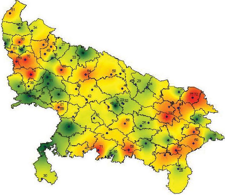
Figure 2(a): TOPSIS method ranking visualization map.
3.6 Visualization of Ranked Districts
It is interesting to observe that MCDM methods provide almost similar ranking for top twenty districts, there is a significant variation is being observed in the ranking of remaining districts. It might be because of the fact that different tools emphasises different criteria. This study found that the Spearman rank correlation coefficient for various pairs of tools is statistically significant with a value of . This implies the relevance of both approaches of ranking. This means the two methods of ranking are highly significant.
Figures 2(a) and 2(b) shows the visualization map of rank districts using the aforesaid methods TOPSIS and MOORA.
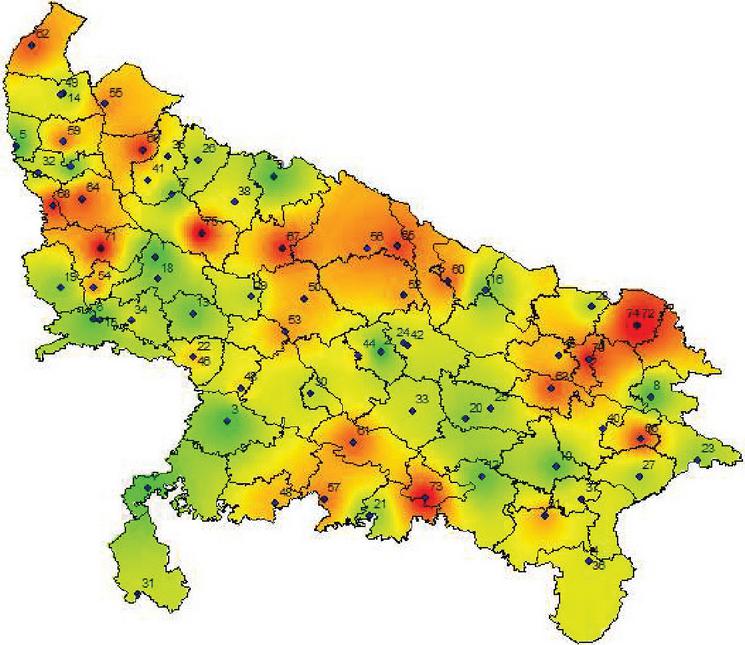
Figure 2(b): MOORA method ranking visualization map.
In the above figures, red colour indicates higher ranked and relatively more vulnerable districts, orange colour indicates districts with moderate vulnerability, yellow colour indicates districts with relatively weaker vulnerability and green colour indicates districts with almost no vulnerability (safe zone).
4 Conclusion
By considering demographic characteristics such as district-wise population, area, female literacy rate, female birth rate and health indicators based on child mortality rate and fertility rates, we motivated to assess the overall performance of different districts in UP and particularly aimed at identifying the districts with significant rankings to bring future improvements. We found the following top ten districts with relatively higher order namely, Sonbhadra, Lalitpur, Jaluan, Agra, Kanpur Nagar, Jhansi, Moradabad, Mirzapur and Hamirpur and the following districts with relatively poorer rankings namely, Bareilly, Sitapur, Allahbad, Aligarh and Lucknow. Though, the TOPSIS method is expected to identify the best-performing districts, whereas, the MOORA method enables us to determine the districts’ optimal ranking based on multiple objectives, in the present scenario both tools become unidirectional. The study revealed that certain districts in UP have excelled in terms of these criteria, while others lag behind. It also highlights the need for targeted interventions and policies in lagging dis to address the underlying challenges and promote inclusive development. It is important to highlight the name of computed outlier’s districts for each of the variables under study as shown in Appendix 4, and requires special investigation to find the underlying causes. In this paper, we statistically evaluated the progress of districts using various demographic indicators filtered through TOPSIS and MOORA methods. It is essential to emphasize the identification of specific outlier districts calculated for different variables under the study, necessitating a thorough examination to uncover the root causes of variability, as depicted in Appendix 4. (Agra, Kanpur Nagar, Moradabad), Lucknow, Shrawasti and are the districts declared outliers in respect to variables like, area, CAW, and TFR respectively. It is interesting to present our researchers, policy and decision-makers and all related stakeholders including common people of the State to bring focused attention and timely intervention to reduce the heterogeneity that persists across all seventy-five districts of UP that is one of the fastest evolving States of India in terms of increasing investment destination, improving laws and order State, a hotspot of religious tourism, and witnessed as one of the fastest growing States of India.
5 Limitations
However, it is important to acknowledge the limitations of the study. The first notifiable limitation is the secondary data source, which was acquired deliberately to ensure the authenticity and reliability of the data set. But, at the same, it didn’t provide us enough scope for survey-based experimentation. The second limitation refers to the methods using TOPSIS and MOORA. As the number of criteria and alternatives increases, there is a corresponding escalation in the computational intricacy and time needed to conduct the analysis. TOPSIS and MOORA approaches necessitate a substantial volume of data to ensure precision in the analysis, a resource that may not be consistently accessible or effortlessly procured.
6 Future Scope
The present work may provide good insight and show the roadmap to future researchers for carrying out the micro-level analysis that consists of relatively smaller geographical units of research namely, sub-divisions, blocks and villages for bringing in-depth investigation and achieving relatively higher precisions. The present work provides a unique understanding of challenges, threats and opportunities in each district of UP. Furthermore, MCDM methodologies such as CRITIC, AHP, MOORA and TOPSIS implementations to evaluate district-specific factors need to be investigated at micro geographical units (sub-divisions, blocks, and villages) of research. Employ information derived from the Census of India, the National Sample Survey Office (NSSO), and various other governmental sources to access current demographic and socio-economic data. In the future, additional demographic variables sourced from existing data could potentially be integrated. As UP is the most populous state of India, the assurance of data availability and reliability at the district level may present challenges arising from discrepancies or deficiencies in data collection and reporting. The varied geographical terrain of UP could potentially give rise to logistical hurdles in the process of data collection and fieldwork.
7 Competing Interests and Funding
The authors declare that they have no conflict of interest and that there is no funding for this research article.
Appendix
Appendix 1: Weighted Normalized Matrix by TOPSIS method
| S.N. | Districts | ||||||||
| 1 | Saharanpur | 0.01496 | 0.01844 | 0.01347 | 0.01566 | 0.01182 | 0.01111 | 0.01442 | 0.01909 |
| 2 | Bijnor | 0.01525 | 0.01716 | 0.01479 | 0.01566 | 0.01403 | 0.01066 | 0.01346 | 0.02027 |
| 3 | Rampur | 0.01193 | 0.01747 | 0.00864 | 0.01210 | 0.00656 | 0.01309 | 0.01866 | 0.01286 |
| 4 | Jyotiba Phule Nagar | 0.01276 | 0.01552 | 0.00821 | 0.00926 | 0.00658 | 0.01307 | 0.01434 | 0.01013 |
| 5 | Meerut | 0.01629 | 0.01671 | 0.00946 | 0.02136 | 0.01218 | 0.01194 | 0.01366 | 0.01896 |
| 6 | Baghpat | 0.01591 | 0.01476 | 0.00482 | 0.00783 | 0.00622 | 0.01165 | 0.01158 | 0.00717 |
| 7 | Gautam Buddha Nagar | 0.01655 | 0.01619 | 0.00527 | 0.01495 | 0.01203 | 0.00792 | 0.01577 | 0.00907 |
| 8 | Bulandshahr | 0.01473 | 0.01518 | 0.01590 | 0.02065 | 0.01969 | 0.01257 | 0.01823 | 0.01926 |
| 9 | Aligarh | 0.01374 | 0.01859 | 0.01333 | 0.02136 | 0.02483 | 0.01215 | 0.01626 | 0.02022 |
| 10 | Mahamaya Nagar | 0.01376 | 0.01785 | 0.00672 | 0.00783 | 0.00708 | 0.01117 | 0.01576 | 0.00861 |
| 11 | Mathura | 0.01335 | 0.01678 | 0.01220 | 0.01566 | 0.01744 | 0.01266 | 0.01468 | 0.01402 |
| 12 | Agra | 0.01288 | 0.01628 | 0.03967 | 0.02848 | 0.01578 | 0.01158 | 0.01890 | 0.02432 |
| 13 | Firozabad | 0.01493 | 0.01572 | 0.00863 | 0.01495 | 0.01417 | 0.01173 | 0.02004 | 0.01375 |
| 14 | Mainpuri | 0.01543 | 0.01510 | 0.01008 | 0.00997 | 0.00891 | 0.01136 | 0.02273 | 0.01197 |
| 15 | Bareilly | 0.01105 | 0.01956 | 0.01504 | 0.02065 | 0.01837 | 0.01041 | 0.01375 | 0.02449 |
| 16 | Pilibhit | 0.01126 | 0.01469 | 0.01278 | 0.01068 | 0.01054 | 0.00982 | 0.01039 | 0.00070 |
| 17 | Shahjahanpur | 0.01190 | 0.01920 | 0.01671 | 0.01638 | 0.01348 | 0.01570 | 0.02367 | 0.01655 |
| 18 | Kheri | 0.01186 | 0.01626 | 0.02804 | 0.01638 | 0.01805 | 0.01205 | 0.02015 | 0.02214 |
| 19 | Sitapur | 0.01122 | 0.01824 | 0.02097 | 0.02065 | 0.01873 | 0.01362 | 0.02162 | 0.02468 |
| 20 | Hardoi | 0.01153 | 0.01980 | 0.02187 | 0.01780 | 0.00959 | 0.01455 | 0.02327 | 0.02253 |
| 21 | Unnao | 0.01341 | 0.01732 | 0.01664 | 0.01495 | 0.01417 | 0.01088 | 0.01555 | 0.01711 |
| 22 | Lucknow | 0.01602 | 0.01770 | 0.00923 | 0.03061 | 0.04418 | 0.00798 | 0.00681 | 0.02527 |
| 23 | Farrukhabad | 0.01321 | 0.01424 | 0.00796 | 0.00997 | 0.00568 | 0.01345 | 0.01653 | 0.01038 |
| 24 | Kannauj | 0.01363 | 0.01873 | 0.00764 | 0.00641 | 0.00776 | 0.01365 | 0.01761 | 0.00757 |
| 25 | Etawah | 0.01605 | 0.01442 | 0.00844 | 0.01495 | 0.00459 | 0.01166 | 0.01577 | 0.00871 |
| 26 | Auraiya | 0.01566 | 0.01588 | 0.00736 | 0.00783 | 0.00712 | 0.01086 | 0.01548 | 0.00759 |
| 27 | Kanpur Dehat | 0.01472 | 0.01853 | 0.01103 | 0.01210 | 0.01156 | 0.01068 | 0.01524 | 0.00989 |
| 28 | Kanpur Nagar | 0.01704 | 0.01473 | 0.03967 | 0.02990 | 0.02385 | 0.00818 | 0.00739 | 0.02522 |
| 29 | Jalaun | 0.01385 | 0.01438 | 0.01659 | 0.01566 | 0.00566 | 0.00898 | 0.00405 | 0.00930 |
| 30 | Jhansi | 0.01459 | 0.01673 | 0.01667 | 0.01851 | 0.01016 | 0.00807 | 0.01145 | 0.01100 |
| 31 | Lalitpur | 0.01157 | 0.01801 | 0.01840 | 0.01068 | 0.00171 | 0.01021 | 0.00275 | 0.00672 |
| 32 | Hamirpur | 0.01456 | 0.01592 | 0.01505 | 0.00997 | 0.00481 | 0.01027 | 0.01408 | 0.00608 |
| 33 | Mahoba | 0.01369 | 0.01906 | 0.01053 | 0.00712 | 0.00321 | 0.01196 | 0.01158 | 0.00482 |
| 34 | Banda | 0.01203 | 0.01752 | 0.01610 | 0.01282 | 0.00763 | 0.01194 | 0.01591 | 0.00991 |
| 35 | Chitrakoot | 0.01167 | 0.01604 | 0.01155 | 0.00712 | 0.00331 | 0.01175 | 0.01222 | 0.00546 |
| 36 | Fatehpur | 0.01301 | 0.01606 | 0.01516 | 0.01424 | 0.00953 | 0.01301 | 0.01409 | 0.01449 |
| 37 | Pratapgarh | 0.01552 | 0.01866 | 0.01362 | 0.01566 | 0.01578 | 0.01048 | 0.01211 | 0.01767 |
| 38 | Kaushambi | 0.01228 | 0.01754 | 0.00650 | 0.00997 | 0.00585 | 0.01336 | 0.01242 | 0.00881 |
| 39 | Allahabad | 0.01383 | 0.02149 | 0.02002 | 0.02919 | 0.02711 | 0.01154 | 0.01528 | 0.03278 |
| 40 | Bara Banki | 0.01173 | 0.01716 | 0.01421 | 0.01638 | 0.01136 | 0.01309 | 0.01509 | 0.01795 |
| 41 | Faizabad | 0.01538 | 0.01597 | 0.00921 | 0.01282 | 0.01212 | 0.01054 | 0.00809 | 0.01360 |
| 42 | Ambedkar Nagar | 0.01591 | 0.01476 | 0.00858 | 0.01353 | 0.00711 | 0.00851 | 0.00940 | 0.01320 |
| 43 | Bahraich | 0.00814 | 0.01530 | 0.01715 | 0.01638 | 0.01424 | 0.01784 | 0.01653 | 0.01920 |
| 44 | Shrawasti | 0.00809 | 0.01752 | 0.00711 | 0.00498 | 0.00436 | 0.01836 | 0.01167 | 0.00614 |
| 45 | Balrampur | 0.00881 | 0.01866 | 0.01223 | 0.01139 | 0.00542 | 0.01800 | 0.01648 | 0.01183 |
| 46 | Gonda | 0.01201 | 0.01754 | 0.01462 | 0.01210 | 0.00934 | 0.01202 | 0.00926 | 0.01890 |
| 47 | Siddharthnagar | 0.01010 | 0.01538 | 0.01057 | 0.01282 | 0.00537 | 0.01520 | 0.00449 | 0.01409 |
| 48 | Basti | 0.01325 | 0.01615 | 0.00982 | 0.01210 | 0.00523 | 0.01134 | 0.00907 | 0.01357 |
| 49 | Sant Kabir Nagar | 0.01282 | 0.01507 | 0.00601 | 0.00641 | 0.00447 | 0.01160 | 0.00722 | 0.00940 |
| 50 | Mahrajganj | 0.01287 | 0.01684 | 0.01078 | 0.01424 | 0.00650 | 0.01048 | 0.00814 | 0.01478 |
| 51 | Gorakhpur | 0.01427 | 0.01617 | 0.01272 | 0.01994 | 0.01390 | 0.01019 | 0.01148 | 0.02445 |
| 52 | Kushinagar | 0.01309 | 0.01949 | 0.01061 | 0.01353 | 0.00784 | 0.01216 | 0.00814 | 0.01962 |
| 53 | Deoria | 0.01490 | 0.01808 | 0.00928 | 0.01638 | 0.00137 | 0.00985 | 0.00457 | 0.01707 |
| 54 | Azamgarh | 0.01593 | 0.01514 | 0.01480 | 0.01851 | 0.01182 | 0.01071 | 0.01318 | 0.02539 |
| 55 | Mau | 0.01498 | 0.01693 | 0.00626 | 0.00854 | 0.00808 | 0.00965 | 0.01444 | 0.01214 |
| 56 | Ballia | 0.01461 | 0.01916 | 0.01089 | 0.02207 | 0.00574 | 0.00948 | 0.00560 | 0.01783 |
| 57 | Jaunpur | 0.01598 | 0.01621 | 0.01475 | 0.01994 | 0.00791 | 0.01010 | 0.00385 | 0.02474 |
| 58 | Ghazipur | 0.01510 | 0.01754 | 0.01233 | 0.01922 | 0.01080 | 0.01051 | 0.00559 | 0.01993 |
| 59 | Chandauli | 0.01473 | 0.01583 | 0.00907 | 0.01139 | 0.00362 | 0.01123 | 0.00814 | 0.01075 |
| 60 | Varanasi | 0.01644 | 0.01597 | 0.00561 | 0.01994 | 0.01680 | 0.00866 | 0.00558 | 0.02024 |
| 61 | Bhadohi | 0.01439 | 0.01514 | 0.00371 | 0.00641 | 0.00304 | 0.01259 | 0.00814 | 0.00869 |
| 62 | Mirzapur | 0.01460 | 0.01465 | 0.01651 | 0.01353 | 0.00445 | 0.01156 | 0.01132 | 0.01375 |
| 63 | Sonbhadra | 0.01275 | 0.01758 | 0.02479 | 0.01566 | 0.00427 | 0.01381 | 0.01161 | 0.01025 |
| 64 | Etah | 0.01405 | 0.01812 | 0.01624 | 0.01282 | 0.00622 | 0.01252 | 0.01562 | 0.00977 |
| 65 | Kanshiram Nagar | 0.01186 | 0.01799 | 0.00728 | 0.00783 | 0.01165 | 0.01535 | 0.01900 | 0.00791 |
| 66 | Amethi | 0.01323 | 0.01523 | 0.00851 | 0.01068 | 0.00486 | 0.01250 | 0.02543 | 0.01028 |
| 67 | Budaun | 0.01018 | 0.01570 | 0.01546 | 0.01566 | 0.00948 | 0.01325 | 0.01600 | 0.01722 |
| 68 | Ghaziabad | 0.01667 | 0.02133 | 0.00378 | 0.01495 | 0.00919 | 0.00872 | 0.00997 | 0.01875 |
| 69 | Hapur | 0.01544 | 0.01418 | 0.00408 | 0.00783 | 0.00286 | 0.01177 | 0.01631 | 0.00737 |
| 70 | Moradabad | 0.01365 | 0.01844 | 0.03967 | 0.01424 | 0.01724 | 0.01100 | 0.01595 | 0.01875 |
| 71 | Muzaffarnagar | 0.01519 | 0.01561 | 0.01092 | 0.01495 | 0.00704 | 0.01037 | 0.00418 | 0.01558 |
| 72 | Rae Bareli | 0.01310 | 0.01572 | 0.01476 | 0.01353 | 0.01088 | 0.01046 | 0.00947 | 0.01598 |
| 73 | Sambhal | 0.01073 | 0.01696 | 0.00896 | 0.00926 | 0.00757 | 0.01397 | 0.01815 | 0.01207 |
| 74 | Shamli | 0.01361 | 0.01857 | 0.00426 | 0.00570 | 0.00433 | 0.01220 | 0.01492 | 0.00723 |
| 75 | Sultanpur | 0.01494 | 0.01799 | 0.00976 | 0.01353 | 0.00967 | 0.01045 | 0.01132 | 0.01339 |
Appendix 2: Normalized Matrix for MOORA
| S.N. | Districts | ||||||||
| 1 | Saharanpur | 0.12559 | 0.12551 | 0.10478 | 0.11762 | 0.11160 | 0.10784 | 0.11860 | 0.13911 |
| 2 | Bijnor | 0.12800 | 0.11679 | 0.11501 | 0.11762 | 0.13240 | 0.10343 | 0.11071 | 0.14775 |
| 3 | Rampur | 0.10014 | 0.11888 | 0.06723 | 0.09089 | 0.06195 | 0.12707 | 0.15351 | 0.09371 |
| 4 | Jyotiba Phule Nagar | 0.10711 | 0.10561 | 0.06388 | 0.06950 | 0.06210 | 0.12690 | 0.11798 | 0.07383 |
| 5 | Meerut | 0.13671 | 0.11372 | 0.07357 | 0.16039 | 0.11497 | 0.11593 | 0.11239 | 0.13817 |
| 6 | Baghpat | 0.13353 | 0.10045 | 0.03752 | 0.05881 | 0.05873 | 0.11309 | 0.09527 | 0.05228 |
| 7 | Gautam Buddha Nagar | 0.13892 | 0.11016 | 0.04096 | 0.11227 | 0.11351 | 0.07687 | 0.12970 | 0.06612 |
| 8 | Bulandshahr | 0.12358 | 0.10328 | 0.12364 | 0.15504 | 0.18586 | 0.12205 | 0.14993 | 0.14039 |
| 9 | Aligarh | 0.11533 | 0.12649 | 0.10367 | 0.16039 | 0.23433 | 0.11795 | 0.13379 | 0.14740 |
| 10 | Mahamaya Nagar | 0.11550 | 0.12145 | 0.05226 | 0.05881 | 0.06679 | 0.10837 | 0.12960 | 0.06278 |
| 11 | Mathura | 0.11204 | 0.11421 | 0.09487 | 0.11762 | 0.16462 | 0.12285 | 0.12075 | 0.10219 |
| 12 | Agra | 0.10809 | 0.11077 | 0.30855 | 0.21385 | 0.14895 | 0.11242 | 0.15547 | 0.17728 |
| 13 | Firozabad | 0.12531 | 0.10696 | 0.06709 | 0.11227 | 0.13372 | 0.11382 | 0.16482 | 0.10023 |
| 14 | Mainpuri | 0.12948 | 0.10279 | 0.07840 | 0.07485 | 0.08407 | 0.11030 | 0.18693 | 0.08726 |
| 15 | Bareilly | 0.09276 | 0.13312 | 0.11702 | 0.15504 | 0.17341 | 0.10101 | 0.11307 | 0.17847 |
| 16 | Pilibhit | 0.09451 | 0.09996 | 0.09939 | 0.08019 | 0.09945 | 0.09533 | 0.08549 | 0.00513 |
| 17 | Shahjahanpur | 0.09991 | 0.13066 | 0.12995 | 0.12296 | 0.12727 | 0.15238 | 0.19474 | 0.12062 |
| 18 | Kheri | 0.09956 | 0.11065 | 0.21814 | 0.12296 | 0.17033 | 0.11691 | 0.16575 | 0.16133 |
| 19 | Sitapur | 0.09414 | 0.12416 | 0.16312 | 0.15504 | 0.17678 | 0.13217 | 0.17787 | 0.17990 |
| 20 | Hardoi | 0.09679 | 0.13472 | 0.17011 | 0.13366 | 0.09051 | 0.14120 | 0.19141 | 0.16421 |
| 21 | Unnao | 0.11250 | 0.11789 | 0.12947 | 0.11227 | 0.13372 | 0.10560 | 0.12788 | 0.12471 |
| 22 | Lucknow | 0.13448 | 0.12047 | 0.07181 | 0.22989 | 0.41697 | 0.07743 | 0.05605 | 0.18415 |
| 23 | Farrukhabad | 0.11087 | 0.09689 | 0.06195 | 0.07485 | 0.05360 | 0.13055 | 0.13597 | 0.07563 |
| 24 | Kannauj | 0.11435 | 0.12747 | 0.05945 | 0.04812 | 0.07323 | 0.13250 | 0.14486 | 0.05520 |
| 25 | Etawah | 0.13469 | 0.09812 | 0.06564 | 0.11227 | 0.04335 | 0.11321 | 0.12971 | 0.06346 |
| 26 | Auraiya | 0.13141 | 0.10807 | 0.05726 | 0.05881 | 0.06722 | 0.10538 | 0.12735 | 0.05535 |
| 27 | Kanpur Dehat | 0.12358 | 0.12612 | 0.08581 | 0.09089 | 0.10911 | 0.10364 | 0.12534 | 0.07206 |
| 28 | Kanpur Nagar | 0.14302 | 0.10021 | 0.30855 | 0.22454 | 0.22511 | 0.07936 | 0.06082 | 0.18380 |
| 29 | Jalaun | 0.11621 | 0.09788 | 0.12907 | 0.11762 | 0.05346 | 0.08719 | 0.03335 | 0.06780 |
| 30 | Jhansi | 0.12244 | 0.11384 | 0.12966 | 0.13900 | 0.09593 | 0.07833 | 0.09417 | 0.08018 |
| 31 | Lalitpur | 0.09711 | 0.12256 | 0.14313 | 0.08019 | 0.01611 | 0.09913 | 0.02265 | 0.04901 |
| 32 | Hamirpur | 0.12220 | 0.10831 | 0.11705 | 0.07485 | 0.04540 | 0.09970 | 0.11586 | 0.04430 |
| 33 | Mahoba | 0.11493 | 0.12968 | 0.08192 | 0.05346 | 0.03032 | 0.11606 | 0.09527 | 0.03514 |
| 34 | Banda | 0.10098 | 0.11924 | 0.12521 | 0.09623 | 0.07206 | 0.11591 | 0.13084 | 0.07219 |
| 35 | Chitrakoot | 0.09791 | 0.10917 | 0.08987 | 0.05346 | 0.03120 | 0.11406 | 0.10056 | 0.03979 |
| 36 | Fatehpur | 0.10916 | 0.10930 | 0.11793 | 0.10693 | 0.08993 | 0.12632 | 0.11588 | 0.10563 |
| 37 | Pratapgarh | 0.13022 | 0.12698 | 0.10595 | 0.11762 | 0.14895 | 0.10174 | 0.09962 | 0.12875 |
| 38 | Kaushambi | 0.10308 | 0.11937 | 0.05056 | 0.07485 | 0.05521 | 0.12970 | 0.10215 | 0.06418 |
| 39 | Allahabad | 0.11603 | 0.14626 | 0.15571 | 0.21920 | 0.25586 | 0.11202 | 0.12570 | 0.23888 |
| 40 | Bara Banki | 0.09842 | 0.11679 | 0.11053 | 0.12296 | 0.10721 | 0.12702 | 0.12410 | 0.13082 |
| 41 | Faizabad | 0.12908 | 0.10868 | 0.07164 | 0.09623 | 0.11438 | 0.10231 | 0.06651 | 0.09914 |
| 42 | Ambedkar Nagar | 0.13356 | 0.10045 | 0.06675 | 0.10158 | 0.06708 | 0.08263 | 0.07732 | 0.09620 |
| 43 | Bahraich | 0.06831 | 0.10414 | 0.13341 | 0.12296 | 0.13445 | 0.17314 | 0.13600 | 0.13993 |
| 44 | Shrawasti | 0.06790 | 0.11924 | 0.05534 | 0.03742 | 0.04115 | 0.17823 | 0.09600 | 0.04472 |
| 45 | Balrampur | 0.07391 | 0.12698 | 0.09513 | 0.08554 | 0.05111 | 0.17466 | 0.13557 | 0.08621 |
| 46 | Gonda | 0.10081 | 0.11937 | 0.11370 | 0.09089 | 0.08817 | 0.11666 | 0.07616 | 0.13777 |
| 47 | Siddharthnagar | 0.08475 | 0.10463 | 0.08223 | 0.09623 | 0.05067 | 0.14756 | 0.03697 | 0.10268 |
| 48 | Basti | 0.11122 | 0.10991 | 0.07635 | 0.09089 | 0.04936 | 0.11010 | 0.07464 | 0.09888 |
| 49 | Sant Kabir Nagar | 0.10759 | 0.10254 | 0.04675 | 0.04812 | 0.04218 | 0.11258 | 0.05937 | 0.06847 |
| 50 | Mahrajganj | 0.10804 | 0.11458 | 0.08385 | 0.10693 | 0.06137 | 0.10168 | 0.06695 | 0.10773 |
| 51 | Gorakhpur | 0.11977 | 0.11003 | 0.09893 | 0.14970 | 0.13123 | 0.09894 | 0.09440 | 0.17817 |
| 52 | Kushinagar | 0.10984 | 0.13263 | 0.08254 | 0.10158 | 0.07396 | 0.11805 | 0.06695 | 0.14301 |
| 53 | Deoria | 0.12501 | 0.12305 | 0.07215 | 0.12296 | 0.01289 | 0.09564 | 0.03757 | 0.12441 |
| 54 | Azamgarh | 0.13365 | 0.10303 | 0.11515 | 0.13900 | 0.11160 | 0.10392 | 0.10841 | 0.18504 |
| 55 | Mau | 0.12568 | 0.11519 | 0.04866 | 0.06416 | 0.07631 | 0.09366 | 0.11874 | 0.08847 |
| 56 | Ballia | 0.12262 | 0.13042 | 0.08467 | 0.16574 | 0.05419 | 0.09198 | 0.04607 | 0.12998 |
| 57 | Jaunpur | 0.13415 | 0.11028 | 0.11470 | 0.14970 | 0.07469 | 0.09806 | 0.03163 | 0.18031 |
| 58 | Ghazipur | 0.12672 | 0.11937 | 0.09592 | 0.14435 | 0.10194 | 0.10200 | 0.04600 | 0.14524 |
| 59 | Chandauli | 0.12364 | 0.10770 | 0.07058 | 0.08554 | 0.03412 | 0.10899 | 0.06695 | 0.07835 |
| 60 | Varanasi | 0.13799 | 0.10868 | 0.04360 | 0.14970 | 0.15861 | 0.08409 | 0.04591 | 0.14752 |
| 61 | Bhadohi | 0.12074 | 0.10303 | 0.02883 | 0.04812 | 0.02871 | 0.12215 | 0.06695 | 0.06332 |
| 62 | Mirzapur | 0.12254 | 0.09972 | 0.12841 | 0.10158 | 0.04203 | 0.11216 | 0.09311 | 0.10018 |
| 63 | Sonbhadra | 0.10701 | 0.11961 | 0.19281 | 0.11762 | 0.04028 | 0.13404 | 0.09551 | 0.07473 |
| 64 | Etah | 0.11789 | 0.12330 | 0.12628 | 0.09623 | 0.05873 | 0.12154 | 0.12846 | 0.07119 |
| 65 | Kanshiram Nagar | 0.09951 | 0.12244 | 0.05661 | 0.05881 | 0.10999 | 0.14903 | 0.15625 | 0.05764 |
| 66 | Amethi | 0.11105 | 0.10365 | 0.06616 | 0.08019 | 0.04584 | 0.12132 | 0.20922 | 0.07493 |
| 67 | Budaun | 0.08544 | 0.10684 | 0.12027 | 0.11762 | 0.08949 | 0.12856 | 0.13165 | 0.12554 |
| 68 | Ghaziabad | 0.13989 | 0.14516 | 0.02937 | 0.11227 | 0.08670 | 0.08461 | 0.08203 | 0.13665 |
| 69 | Hapur | 0.12961 | 0.09652 | 0.03170 | 0.05881 | 0.02695 | 0.11422 | 0.13414 | 0.05368 |
| 70 | Moradabad | 0.11456 | 0.12551 | 0.30855 | 0.10693 | 0.16272 | 0.10677 | 0.13122 | 0.13665 |
| 71 | Muzaffarnagar | 0.12744 | 0.10623 | 0.08496 | 0.11227 | 0.06649 | 0.10069 | 0.03440 | 0.11353 |
| 72 | Rae Bareli | 0.10995 | 0.10696 | 0.11484 | 0.10158 | 0.10267 | 0.10153 | 0.07786 | 0.11649 |
| 73 | Sambhal | 0.09003 | 0.11544 | 0.06968 | 0.06950 | 0.07147 | 0.13556 | 0.14927 | 0.08798 |
| 74 | Shamli | 0.11423 | 0.12637 | 0.03316 | 0.04277 | 0.04086 | 0.11841 | 0.12274 | 0.05270 |
| 75 | Sultanpur | 0.12541 | 0.12244 | 0.07592 | 0.10158 | 0.09124 | 0.10141 | 0.09311 | 0.09755 |
Appendix 3: Presents a normalized matrix evaluated using Equation (11)
| S.N. | Districts | TOPSIS | MOORA |
| 1 | Agra | 4 | 6 |
| 2 | Aligarh | 74 | 71 |
| 3 | Allahabad | 73 | 63 |
| 4 | Ambedkar Nagar | 25 | 20 |
| 5 | Amethi | 55 | 69 |
| 6 | Auraiya | 41 | 43 |
| 7 | Azamgarh | 59 | 46 |
| 8 | Baghpat | 37 | 40 |
| 9 | Bahraich | 65 | 75 |
| 10 | Ballia | 10 | 5 |
| 11 | Balrampur | 29 | 60 |
| 12 | Banda | 15 | 23 |
| 13 | Bara Banki | 46 | 52 |
| 14 | Bareilly | 71 | 57 |
| 15 | Basti | 23 | 24 |
| 16 | Bhadohi | 33 | 38 |
| 17 | Bijnor | 58 | 45 |
| 18 | Budaun | 34 | 55 |
| 19 | Bulandshahr | 70 | 64 |
| 20 | Chandauli | 18 | 17 |
| 21 | Chitrakoot | 16 | 21 |
| 22 | Deoria | 12 | 8 |
| 23 | Etah | 11 | 18 |
| 24 | Etawah | 21 | 22 |
| 25 | Faizabad | 43 | 29 |
| 26 | Farrukhabad | 44 | 61 |
| 27 | Fatehpur | 26 | 34 |
| 28 | Firozabad | 69 | 68 |
| 29 | Gautam Buddha Nagar | 53 | 32 |
| 30 | Ghaziabad | 60 | 27 |
| 31 | Ghazipur | 24 | 16 |
| 32 | Gonda | 31 | 39 |
| 33 | Gorakhpur | 63 | 47 |
| 34 | Hamirpur | 9 | 11 |
| 35 | Hapur | 40 | 50 |
| 36 | Hardoi | 39 | 54 |
| 37 | Jalaun | 3 | 3 |
| 38 | Jaunpur | 19 | 10 |
| 39 | Jhansi | 6 | 7 |
| 40 | Jyotiba Phule Nagar | 42 | 53 |
| 41 | Kannauj | 54 | 58 |
| 42 | Kanpur Dehat | 35 | 30 |
| 43 | Kanpur Nagar | 5 | 1 |
| 44 | Kanshiram Nagar | 68 | 73 |
| 45 | Kaushambi | 32 | 42 |
| 46 | Kheri | 50 | 56 |
| 47 | Kushinagar | 36 | 31 |
| 48 | Lalitpur | 2 | 2 |
| 49 | Lucknow | 75 | 74 |
| 50 | Mahamaya Nagar | 47 | 48 |
| 51 | Mahoba | 14 | 13 |
| 52 | Mahrajganj | 20 | 19 |
| 53 | Mainpuri | 62 | 66 |
| 54 | Mathura | 66 | 59 |
| 55 | Mau | 57 | 51 |
| 56 | Meerut | 52 | 35 |
| 57 | Mirzapur | 8 | 14 |
| 58 | Moradabad | 7 | 9 |
| 59 | Muzaffarnagar | 17 | 12 |
| 60 | Pilibhit | 13 | 15 |
| 61 | Pratapgarh | 56 | 33 |
| 62 | Rae Bareli | 27 | 26 |
| 63 | Rampur | 51 | 62 |
| 64 | Saharanpur | 49 | 41 |
| 65 | Sambhal | 61 | 70 |
| 66 | Sant Kabir Nagar | 28 | 36 |
| 67 | Shahjahanpur | 64 | 67 |
| 68 | Shamli | 45 | 49 |
| 69 | Shrawasti | 38 | 65 |
| 70 | Siddharthnagar | 22 | 28 |
| 71 | Sitapur | 72 | 72 |
| 72 | Sonbhadra | 1 | 4 |
| 73 | Sultanpur | 30 | 25 |
| 74 | Unnao | 48 | 44 |
| 75 | Varanasi | 67 | 37 |
Appendix 4: Z-Scores of the variables
| S.N. | District | A | A | A | A | A | A | A | A |
| 1 | Saharanpur | 0.677 | 0.935 | 0.073 | 0.237 | 0.238 | -0.276 | 0.261 | 0.719 |
| 2 | Bijnor | 0.821 | 0.165 | 0.252 | 0.237 | 0.563 | -0.487 | 0.074 | 0.907 |
| 3 | Rampur | -0.845 | 0.349 | -0.585 | -0.398 | -0.538 | 0.646 | 1.088 | -0.268 |
| 4 | Jyotiba Phule Nagar | -0.428 | -0.822 | -0.644 | -0.906 | -0.536 | 0.638 | 0.246 | -0.701 |
| 5 | Meerut | 1.342 | -0.106 | -0.474 | 1.254 | 0.290 | 0.112 | 0.114 | 0.699 |
| 6 | Baghpat | 1.152 | -1.278 | -1.106 | -1.160 | -0.588 | -0.024 | -0.292 | -1.170 |
| 7 | Gautam Buddha Nagar | 1.474 | -0.421 | -1.045 | 0.110 | 0.267 | -1.760 | 0.524 | -0.869 |
| 8 | Bulandshahr | 0.557 | -1.028 | 0.404 | 1.126 | 1.398 | 0.405 | 1.003 | 0.747 |
| 9 | Aligarh | 0.063 | 1.022 | 0.054 | 1.254 | 2.155 | 0.209 | 0.621 | 0.899 |
| 10 | Mahamaya Nagar | 0.074 | 0.577 | -0.847 | -1.160 | -0.462 | -0.250 | 0.522 | -0.941 |
| 11 | Mathura | -0.133 | -0.063 | -0.101 | 0.237 | 1.066 | 0.443 | 0.312 | -0.084 |
| 12 | Agra | -0.369 | -0.367 | 3.645 | 2.524 | 0.821 | -0.056 | 1.135 | 1.549 |
| 13 | Firozabad | 0.660 | -0.703 | -0.587 | 0.110 | 0.583 | 0.011 | 1.356 | -0.127 |
| 14 | Mainpuri | 0.910 | -1.072 | -0.389 | -0.779 | -0.192 | -0.158 | 1.881 | -0.409 |
| 15 | Bareilly | -1.286 | 1.608 | 0.288 | 1.126 | 1.203 | -0.603 | 0.130 | 1.575 |
| 16 | Pilibhit | -1.181 | -1.321 | -0.021 | -0.652 | 0.048 | -0.875 | -0.524 | -2.195 |
| 17 | Shahjahanpur | -0.858 | 1.391 | 0.514 | 0.364 | 0.483 | 1.859 | 2.066 | 0.317 |
| 18 | Kheri | -0.880 | -0.378 | 2.060 | 0.364 | 1.155 | 0.159 | 1.379 | 1.202 |
| 19 | Sitapur | -1.204 | 0.816 | 1.096 | 1.126 | 1.256 | 0.890 | 1.666 | 1.606 |
| 20 | Hardoi | -1.045 | 1.749 | 1.218 | 0.618 | -0.092 | 1.323 | 1.987 | 1.265 |
| 21 | Unnao | -0.105 | 0.263 | 0.506 | 0.110 | 0.583 | -0.383 | 0.481 | 0.406 |
| 22 | Lucknow | 1.209 | 0.490 | -0.505 | 2.905 | 5.008 | -1.733 | -1.222 | 1.699 |
| 23 | Farrukhabad | -0.203 | -1.592 | -0.677 | -0.779 | -0.668 | 0.812 | 0.673 | -0.662 |
| 24 | Kannauj | 0.005 | 1.109 | -0.721 | -1.414 | -0.362 | 0.906 | 0.883 | -1.106 |
| 25 | Etawah | 1.221 | -1.484 | -0.613 | 0.110 | -0.828 | -0.018 | 0.524 | -0.926 |
| 26 | Auraiya | 1.025 | -0.605 | -0.760 | -1.160 | -0.456 | -0.394 | 0.468 | -1.103 |
| 27 | Kanpur Dehat | 0.557 | 0.989 | -0.259 | -0.398 | 0.199 | -0.477 | 0.421 | -0.739 |
| 28 | Kanpur Nagar | 1.719 | -1.300 | 3.645 | 2.778 | 2.011 | -1.640 | -1.109 | 1.691 |
| 29 | Jalaun | 0.116 | -1.506 | 0.499 | 0.237 | -0.671 | -1.265 | -1.760 | -0.832 |
| 30 | Jhansi | 0.489 | -0.095 | 0.509 | 0.745 | -0.007 | -1.690 | -0.318 | -0.563 |
| 31 | Lalitpur | -1.026 | 0.675 | 0.745 | -0.652 | -1.254 | -0.693 | -2.014 | -1.241 |
| 32 | Hamirpur | 0.474 | -0.584 | 0.288 | -0.779 | -0.796 | -0.666 | 0.196 | -1.343 |
| 33 | Mahoba | 0.040 | 1.304 | -0.328 | -1.287 | -1.032 | 0.118 | -0.292 | -1.542 |
| 34 | Banda | -0.795 | 0.382 | 0.431 | -0.271 | -0.380 | 0.111 | 0.551 | -0.737 |
| 35 | Chitrakoot | -0.978 | -0.508 | -0.188 | -1.287 | -1.018 | 0.022 | -0.167 | -1.441 |
| 36 | Fatehpur | -0.306 | -0.497 | 0.304 | -0.017 | -0.101 | 0.610 | 0.196 | -0.009 |
| 37 | Pratapgarh | 0.954 | 1.065 | 0.094 | 0.237 | 0.821 | -0.568 | -0.189 | 0.494 |
| 38 | Kaushambi | -0.669 | 0.393 | -0.877 | -0.779 | -0.643 | 0.772 | -0.129 | -0.911 |
| 39 | Allahabad | 0.105 | 2.768 | 0.966 | 2.651 | 2.491 | -0.076 | 0.429 | 2.889 |
| 40 | Bara Banki | -0.948 | 0.165 | 0.174 | 0.364 | 0.169 | 0.643 | 0.391 | 0.539 |
| 41 | Faizabad | 0.885 | -0.551 | -0.508 | -0.271 | 0.281 | -0.541 | -0.974 | -0.150 |
| 42 | Ambedkar Nagar | 1.153 | -1.278 | -0.593 | -0.144 | -0.458 | -1.484 | -0.718 | -0.214 |
| 43 | Bahraich | -2.748 | -0.952 | 0.575 | 0.364 | 0.595 | 2.854 | 0.673 | 0.737 |
| 44 | Shrawasti | -2.772 | 0.382 | -0.793 | -1.669 | -0.863 | 3.097 | -0.275 | -1.334 |
| 45 | Balrampur | -2.413 | 1.065 | -0.096 | -0.525 | -0.707 | 2.926 | 0.663 | -0.432 |
| 46 | Gonda | -0.805 | 0.393 | 0.230 | -0.398 | -0.128 | 0.147 | -0.745 | 0.690 |
| 47 | Siddharthnagar | -1.765 | -0.909 | -0.322 | -0.271 | -0.714 | 1.628 | -1.674 | -0.073 |
| 48 | Basti | -0.182 | -0.443 | -0.425 | -0.398 | -0.735 | -0.167 | -0.781 | -0.156 |
| 49 | Sant Kabir Nagar | -0.399 | -1.093 | -0.944 | -1.414 | -0.847 | -0.049 | -1.143 | -0.817 |
| 50 | Mahrajganj | -0.373 | -0.030 | -0.294 | -0.017 | -0.547 | -0.571 | -0.964 | 0.037 |
| 51 | Gorakhpur | 0.329 | -0.432 | -0.029 | 0.999 | 0.544 | -0.702 | -0.313 | 1.569 |
| 52 | Kushinagar | -0.265 | 1.564 | -0.317 | -0.144 | -0.350 | 0.213 | -0.964 | 0.804 |
| 53 | Deoria | 0.642 | 0.718 | -0.499 | 0.364 | -1.304 | -0.860 | -1.660 | 0.399 |
| 54 | Azamgarh | 1.159 | -1.050 | 0.255 | 0.745 | 0.238 | -0.464 | 0.019 | 1.718 |
| 55 | Mau | 0.682 | 0.024 | -0.910 | -1.033 | -0.314 | -0.955 | 0.264 | -0.382 |
| 56 | Ballia | 0.499 | 1.369 | -0.279 | 1.381 | -0.659 | -1.036 | -1.459 | 0.520 |
| 57 | Jaunpur | 1.188 | -0.410 | 0.247 | 0.999 | -0.339 | -0.744 | -1.801 | 1.615 |
| 58 | Ghazipur | 0.744 | 0.393 | -0.082 | 0.872 | 0.087 | -0.556 | -1.460 | 0.852 |
| 59 | Chandauli | 0.560 | -0.638 | -0.526 | -0.525 | -0.973 | -0.221 | -0.964 | -0.603 |
| 60 | Varanasi | 1.418 | -0.551 | -0.999 | 0.999 | 0.972 | -1.414 | -1.462 | 0.902 |
| 61 | Sant Ravidas Nagar (Bhadohi) | 0.387 | -1.050 | -1.258 | -1.414 | -1.057 | 0.410 | -0.964 | -0.930 |
| 62 | Mirzapur | 0.495 | -1.343 | 0.487 | -0.144 | -0.849 | -0.069 | -0.343 | -0.128 |
| 63 | Sonbhadra | -0.434 | 0.414 | 1.616 | 0.237 | -0.877 | 0.980 | -0.287 | -0.681 |
| 64 | Etah | 0.217 | 0.740 | 0.450 | -0.271 | -0.588 | 0.381 | 0.495 | -0.758 |
| 65 | Kanshiram Nagar | -0.882 | 0.664 | -0.771 | -1.160 | 0.213 | 1.698 | 1.153 | -1.053 |
| 66 | Amethi | -0.192 | -0.996 | -0.604 | -0.652 | -0.790 | 0.370 | 2.409 | -0.677 |
| 67 | Budaun | -1.723 | -0.714 | 0.345 | 0.237 | -0.108 | 0.717 | 0.570 | 0.424 |
| 68 | Ghaziabad | 1.532 | 2.671 | -1.248 | 0.110 | -0.151 | -1.389 | -0.606 | 0.666 |
| 69 | Hapur | 0.917 | -1.625 | -1.208 | -1.160 | -1.085 | 0.030 | 0.629 | -1.139 |
| 70 | Moradabad | 0.018 | 0.935 | 3.645 | -0.017 | 1.036 | -0.327 | 0.560 | 0.666 |
| 71 | Muzaffarnagar | 0.788 | -0.768 | -0.274 | 0.110 | -0.467 | -0.619 | -1.735 | 0.163 |
| 72 | Rae Bareli | -0.258 | -0.703 | 0.249 | -0.144 | 0.098 | -0.578 | -0.705 | 0.227 |
| 73 | Sambhal | -1.449 | 0.046 | -0.542 | -0.906 | -0.389 | 1.053 | 0.988 | -0.393 |
| 74 | Shamli | -0.002 | 1.011 | -1.182 | -1.541 | -0.867 | 0.231 | 0.359 | -1.160 |
| 75 | Sultanpur | 0.666 | 0.664 | -0.433 | -0.144 | -0.080 | -0.584 | -0.343 | -0.185 |
References
[1] A. W., and P. D. Coat, “Decision analysis: A Bayesian approach, Journal of the Royal Statistical Society,” Journal of the Royal Statistical Society, 29(2), 207–224, 1960.
[2] C. A. Howard, “Dynamic programming and Markov processes,” John Wiley, 1960.
[3] H. Kazan and O. Ozdemir, “Financial Performance Assessment of Large Scale Conglomerates Via Topsis and Critic Methods,” International Journal of Management and Sustainability, vol. 3, no. 4, pp. 203–224, Mar. 2014, doi: 10.18488/journal.11/2014.3.4/11.4.203.224.
[4] A. R. Krishnan, M. M. Kasim, R. Hamid, and M. F. Ghazali, “A modified critic method to estimate the objective weights of decision criteria,” Symmetry (Basel), vol. 13, no. 6, Jun. 2021, doi: 10.3390/sym13060973.
[5] H. Deng, C.-H. Yeh, and R. J. Willis, “Inter-company comparison using modified TOPSIS with objective weights,” 2000.
[6] P. Saxena, V. Kumar, and M. Ram, “A novel CRITIC-TOPSIS approach for optimal selection of software reliability growth model (SRGM),” Qual Reliab Eng Int, vol. 38, no. 5, pp. 2501–2520, Jul. 2022, doi: 10.1002/qre.3087.
[7] O. Önay and B. Fatih Yıldırım, “Evaluation of NUTS Level 2 Regions of Turkey by TOPSIS, MOORA and VIKOR 1,” 2016. [Online]. Available: www.ijhssnet.com.
[8] M. O. Esangbedo and J. Wei, “Grey hybrid normalization with period based entropy weighting and relational analysis for cities rankings,” Sci Rep, vol. 13, no. 1, Dec. 2023, doi: 10.1038/s41598-023-40954-4.
[9] M. Behzadian, S. Khanmohammadi Otaghsara, M. Yazdani, and J. Ignatius, “A state-of the-art survey of TOPSIS applications,” Expert Systems with Applications, vol. 39, no. 17. Elsevier Ltd, pp. 13051–13069, Dec. 01, 2012. doi: 10.1016/j.eswa.2012.05.056.
[10] C. Oluah, E. T. Akinlabi, and H. O. Njoku, “Selection of phase change material for improved performance of Trombe wall systems using the entropy weight and TOPSIS methodology,” Energy Build, vol. 217, Jun. 2020, doi: 10.1016/j.enbuild.2020.109967.
[11] H. Ture, S. Dogan, and D. Kocak, “Assessing Euro 2020 Strategy Using Multi-criteria Decision Making Methods: VIKOR and TOPSIS,” Soc Indic Res, vol. 142, no. 2, pp. 645–665, Apr. 2019, doi: 10.1007/s11205-018-1938-8.
[12] H. R. Sama, S. V. K. Kosuri, and S. Kalvakolanu, “Evaluating and ranking the Indian private sector banks—A multi-criteria decision-making approach,” J Public Aff, vol. 22, no. 2, May 2022, doi: 10.1002/pa.2419.
[13] L. Pérez-Domínguez, K. Y. Sánchez Mojica, L. C. Ovalles Pabón, and M. C. Cordero Diáz, “Application of the MOORA method for the evaluation of the industrial maintenance system,” in Journal of Physics: Conference Series, Institute of Physics Publishing, Dec. 2018. doi: 10.1088/1742-6596/1126/1/012018.
[14] L. Pérez-Domínguez, L. A. Rodríguez-Picón, A. Alvarado-Iniesta, D. Luviano Cruz, and Z. Xu, “MOORA under Pythagorean Fuzzy Set for Multiple Criteria Decision Making,” Complexity, vol. 2018, Apr. 2018, doi: 10.1155/2018/2602376.
[15] S. Hajduk and D. Jelonek, “A decision-making approach based on topsis method for ranking smart cities in the context of urban energy,” Energies (Basel), vol. 14, no. 9, May 2021, doi: 10.3390/en14092691.
[16] V. Kumar, P. Saxena, and H. Garg, “Selection of optimal software reliability growth models using an integrated entropy–Technique for Order Preference by Similarity to an Ideal Solution (TOPSIS) approach,” in Mathematical Methods in the Applied Sciences, John Wiley and Sons Ltd, 2021. doi: 10.1002/mma.7445.
[17] “Population Dynamics and Health Issues in India-Final 20-6-22 GO Print ke liye (1).” [Online]. Available: https:/www.researchgate.net/publication/362018745.
[18] I. I. Meshram, N. Kumar Boiroju, V. Kodali, and N. B. Kumar, “Ranking of districts in Andhra Pradesh using women and children nutrition and health indicators by topsis method Corresponding Author Citation Article Cycle,” 2017.
[19] A. Sotoudeh-Anvari, “The applications of MCDM methods in COVID-19 pandemic: A state of the art review,” Applied Soft Computing, vol. 126. Elsevier Ltd, Sep. 01, 2022. doi: 10.1016/j.asoc.2022.109238.
[20] N. Saleh, M. N. Gaber, M. A. Eldosoky, and A. M. Soliman, “Vendor evaluation platform for acquisition of medical equipment based on multi-criteria decision-making approach,” Sci Rep, vol. 13, no. 1, Dec. 2023, doi: 10.1038/s41598-023-38902-3.
[21] “National Family Health Survey (NFHS), 2021, https:/dhsprogram.com.”
[22] D. Diakoulaki, G. Mavrotas, and L. Papayannakis, “Determining Objective Weights in Multiple Criteria Problems: The Critic Method,” 1995.
[23] Hongtao Shi, Yifan Li, Zhongnan Jiang, and Jia Yan, “Comprehensive Evaluation of Power Quality for Microgrid Based on CRITIC Method,” in International Conference on Power Electronics and Motion Control (IPEMC), Nanjing, China.
[24] C. L. Hwang and K. Yoon, “Methods for Multiple Attribute Decision Making. In: Multiple Attribute Decision Making,” Economics and Mathematical Systems.
[25] A. Alinezhad and J. Khalili, “International Series in Operations Research & Management Science New Methods and Applications in Multiple Attribute Decision Making (MADM).” [Online]. Available: http://www.springer.com/series/6161.
Biographies

Sumedha Sharma is pursuing Ph. D. in Statistics from Amity University Uttar Pradesh (AUUP), Noida and also working as a visiting faculty of statistical sciences in the same department. She had rendered services to ICMR Community Cervical Cancer project named “Screening for Cancer of Cervix by Aided-Visual and HPV Tests in a Rural Community” as Assistant Statistician and worked with MoHUPA as a Research Analyst. She gave training with DES, State/UTs on building permit data.

Jitendra Kumar [PhD(Statistics), M.Sc.(Statistics), M. Tech. CSE(AI & ML), FRSS(UK)] is the Associate Professor of Mathematical Statistics, Statistical Sciences and Computational Intelligence (Scientific Computing, Artificial Intelligence, Machine Learning & Quantum Computing), in the Department of Mathematics, School of Advanced Sciences (SAS), Vellore Institute of Technology, Vellore, Tamil Nadu, India(Since Nov 30, 2018 till date). He has been credited to have over 25 years of experiences in academics, research and industry. He had served various organizations namely Prophecy Technology, Gurugram, Datanet India Pvt. Ltd., New Delhi, CSC Pvt. Ltd., New Delhi, Bio Informatics Institute of India, Noida, Caechet Pharmaceutical Pvt. Ltd, Bhiwadi, Rajasthan and some other establishments as Consultant Technical Analyst and Statistician. He had served Amity University Uttar Pradesh (AUUP), Noida (ABS & AIAS) for 13 years (From Jan 13, 2006 to Nov 27, 2018) including Amity University, Dubai Campus (in Yr. 2013) as Assistant Professor (Gr. III.). Dr. Kumar has authored and co-authored few books & contributed many book chapters, over 50 publications, guided over 200 students dissertations & master thesis, supervising six research scholars, reviewed more than 100 research article’s published in reputed Scopus indexed journals, delivered over hundred talks besides being the members of many national and international organizations.

Niraj Kumar Singh has received his Ph. D. in Statistics from Banaras Hindu University in 2012. Presently he is working in Amity University, Noida as an Assistant Professor. He has been credited with 30 publications in mathematical demography and applied statistics. He has served as a reviewer for many peers reviewed and reputed journals.

Anup Kumar had pursued Ph. D. in Statistics from Banaras Hindu University, Varanasi, India. He has worked in Stochastic Modelling of Human fertility (Mathematical Demography). After teaching in the core department of Statistics at Central University of Rajasthan and Allahabad University, switched to Biostatistics Department, SGPGIMS, Lucknow. Dr. Anup has published more than 30 research articles in the area of Mathematical demography and Biostatistics. He has served as reviewer for many peer reviewed and reputed journals.
Journal of Reliability and Statistical Studies, Vol. 17, Issue 1 (2024), 191–222.
doi: 10.13052/jrss0974-8024.1718
© 2024 River Publishers