Incorporating Honey Badger Algorithm in Estimating Gamma Distribution With Application to Stock Price Modelling
Hamza Abubakar1, 2,*, Amani Idris Ahmed Sayed3 and Kamarun Hizam bin Mansor1
1School of Quantitative Sciences, Universiti Utara Malaysia. 06010 Sintok Kedah DarulAman, Malaysia
2Department of Mathematics, Isa Kaita College of Education, Dutsin-ma, Katsina
3Department of Mathematics, Jazan University, 45142 Jizan, Saudi Arabia
E-mail: zeeham4u2c@yahoo.com
*Corresponding Author
Received 23 March 2024; Accepted 02 July 2024
Abstract
This study evaluates the performance of various estimation methods in stock price analysis across diverse parameters, focusing on the Honey Badger Algorithm (HBA). The purpose is to determine the most accurate and reliable method for parameter estimation. Methodologically, we analyze data spanning eight years from publicly traded Malaysian property companies, employing financial metrics such as Mean Absolute Error (MAE) and Root Mean Square Error (RMSE). Our findings highlight HBA’s consistent precision in parameter estimation, with values closely aligning with initial parameters across different stock sizes. For example, HBA-Gamma model achieves an MAE of 0.0592 and an RMSE of 0.8458 for 13 stocks, demonstrating its proficiency in capturing stock price distributions in dynamic markets. In contrast, the Artificial Immune System (AIS) provides reasonable estimates but with higher variability. The Regression Method exhibits mixed outcomes, displaying accuracy in some cases but notable variability and reduced precision, especially with larger datasets. The Moment Method, while adequate, shows slightly higher variance compared to both HBA and AIS. Further analysis using Log Likelihood values confirms HBA’s superior fit to the data, consistently surpassing AIS, Regression Method, and Moment Method in likelihood maximization across various stock numbers. Specifically, HBA exhibits lower MAE and RMSE values of 0.1034 and 0.06723, respectively, for 26 stocks, further validating its effectiveness in parameter estimation and stock price prediction. These findings underscore the importance of integrated approaches that account for market nuances rather than relying solely on individual model forecasts. The results affirm HBA’s potential for informed investment decision-making, emphasizing its robust performance and enhanced predictive capabilities compared to alternative methodologies. However, further research is needed to assess the generalizability of these findings to other markets and contexts.
Keywords: Honey badger algorithm, artificial immune system, stock price, gamma distribution, moment method, regression method.
1 Introduction
In the field of statistical modeling, the ability to identify pivotal data that underpins accurate predictions is crucial (Darrah et al., 2017). With the proliferation of extensive datasets in modern research, scholars are increasingly challenged to construct models and forecast outcomes across diverse real-world contexts. This task is further complicated by the need to sift through noise and extract meaningful patterns that drive decision-making processes.
Fortunately, a broad spectrum of analytical techniques spanning multiple disciplines offers invaluable solutions to researchers seeking profound insights from their data. These techniques include traditional statistical methods, machine learning algorithms, and advanced data mining approaches (Gregova et al., 2020; Jiang, 2020; Mannering et al., 2020; Rajula et al., 2020). Each method brings unique strengths, allowing researchers to tailor their analyses to the specific characteristics and complexities of their datasets.
Stock price prediction and forecasting are pivotal in financial markets, providing essential insights for investors, traders, and financial analysts (Abubakar and Sabri, 2023; Rouf et al., 2021). These tools are indispensable for market participants navigating investment decisions, risk management, and portfolio optimization. Accurate forecasting empowers stakeholders to make informed decisions based on reliable projections, enabling them to seize opportunities, hedge risks effectively, and enhance overall portfolio performance (Harel and Harpaz, 2021; Mondal et al., 2014)
In the dynamic and often unpredictable landscape of financial markets, the importance of precise predictions cannot be overstated (Sornette, 2003).. Market participants rely on these predictions to capitalize on market trends, identify potential pitfalls, and strategically allocate resources. Accurate stock price forecasts provide a strategic advantage, allowing investors to maximize returns and minimize losses in a rapidly changing environment (Figlewski, 1997; Plummer, 2009; Siegel, 2021).
The significance of stock price prediction spans several domains for informed decision-making process, investors rely on stock price forecasts to guide decisions about buying, selling, or holding stocks (Rao and Hossain, 2024). Accurate predictions shape investment strategies and portfolio management. In risk and portfolio management is use for forecasting stock prices helps investors assess and mitigate risks associated with their investments (Abubakar and Muhammad Sabri, 2021; Abubakar and Sabri, 2022). Predictive models enable investors to optimize their portfolios by identifying opportunities for diversification and asset allocation, enhancing returns while minimizing risk (Abubakar and Sabri, 2021; Paiva et al., 2019). In the market efficiency and economic analysis, stock price prediction contributes to market efficiency by ensuring asset prices reflect all available information (S. Ali et al., 2018). Accurate forecasts reduce inefficiencies in asset pricing and promote market liquidity. They also offer insights into broader economic trends, serving as leading indicators of economic activity and sentiment (Schindele et al., 2020).
Traditional modeling techniques often struggle to capture the intricacies of financial systems, leading to suboptimal predictions. Recently, metaheuristic algorithms have gained traction in financial modeling due to their ability to address these challenges (G. A. Ali et al., 2023; Marso and El Merouani, 2020; Mousapour Mamoudan et al., 2023; Shahvaroughi Farahani and Razavi Hajiagha, 2021). Inspired by natural processes like evolution and swarm intelligence, these algorithms offer innovative approaches to parameter estimation and optimization, making them well-suited for handling complex financial data (Janga Reddy and Nagesh Kumar, 2020).
Recent advancements in optimization algorithms have highlighted the Honey Badger Algorithm (HBA) as a significant development (Hashim et al., 2022). The HBA integrates adaptive learning and optimization techniques, facilitating efficient exploration and exploitation of the solution space. This capability is particularly critical in modeling statistical distributions essential for investment decision-making, where high accuracy and precision are paramount. Utilizing the HBA enables financial analysts to enhance predictive models, thereby improving the quality of investment decisions in volatile markets.
Integrating the gamma distribution with the Honey Badger Algorithm leverages the strengths of both statistical modeling and computational intelligence. The gamma distribution, extensively used in finance for modeling asset returns due to its ability to capture skewness and kurtosis, is employed in this context context (Van Tran and Kukal, 2024). Concurrently, the Honey Badger Algorithm, inspired by the resilient and adaptable nature of honey badgers, serves as a robust optimization framework capable of managing complex and dynamic data environments (Hashim et al., 2022). This synergistic integration is anticipated to enhance the accuracy and robustness of predictive models in the financial domain. By combining the statistical properties of the gamma distribution with the adaptive optimization capabilities of the Honey Badger Algorithm, stakeholders are equipped with more reliable and actionable insights for making informed financial decisions (Giannakopoulos et al., 2024; How et al., 2020). This innovative fusion represents a substantial advancement in predictive analytics within finance, empowering stakeholders with superior decision-making capabilities. This research investigates the efficacy of the HBA in estimating gamma distribution parameters and its implications for stock price modeling. The study aims to: (1) Assess the HBA’s effectiveness in parameter estimation for gamma distributions, particularly in modeling stock price dynamics; (2) Benchmark the accuracy and predictive capabilities of the HBA against other methods such as the Artificial Immune System (AIS) and traditional moment methods; and (3) Examine how improved parameter estimation influences investment strategies and portfolio management. By addressing these objectives, this research aspires to advance predictive modeling techniques in finance, providing valuable insights for investors and financial practitioners.
The structure of this paper is presented as follows: Section 2 discusses the Materials and Methods, which include the Gamma Distribution model, the proposed Honey Badger Algorithm (HBA) for parameter estimation, the Artificial Immune System (AIS), and the experimental setup. Section 3 covers the results and discussion, including an analysis of investment risks and returns based on stock price mean, variance, and log-likelihood. Finally, the research is concluded in Section 4.
2 Materials and Methods
2.1 Gamma Distribution
The Gamma distribution, a fundamental probability distribution, is widely applied across diverse domains, showcasing its versatility in modelling various stochastic processes. This distribution effectively represents the time elapsed until an event occurs, making it indispensable in fields like reliability engineering, survival analysis, and queueing theory. It offers a flexible framework for modelling continuous random variables (Kamalov and Denisov, 2020, 2020; Khan et al., 2021). One of its standout features is its ability to accommodate skewed data distributions, making it a preferred choice for scenarios with prominent data asymmetry. Unlike the Normal distribution, which is symmetric, the Gamma distribution’s inherent asymmetry makes it particularly well-suited for applications where positive skewness is prevalent such as financial data (Pekár and Pèolár, 2022). The Gamma distribution is defined by its probability density function (PDF) and cumulative distribution function (CDF) as follows,
| (1) | ||
| (2) |
In this equation, represents the random variable, and are the shape and rate parameters, respectively, denotes the gamma function. is the lower incomplete gamma function. Its shape parameter governs the distribution’s shape, while the rate parameter determines its scale, allowing for tailored representation of a wide range of phenomena.
The survival function, denoted as , is complementary to the CDF and represents the probability that the random variable exceeds a certain value :
| (3) |
The mean and variance of the Gamma distribution can be expressed as follows:
| (4) | |
| (5) |
The likelihood function for a given set of observations can be expressed as the product of the individual probability density functions:
| (6) |
Gamma distribution has been simplifies as,
| (7) |
Taking the logarithm of the likelihood function yields the log-likelihood function, which simplifies computations and is often utilized in parameter estimation:
| (8) |
The Gamma distribution’s versatility makes it invaluable in fields like finance, insurance, engineering, and environmental science. It effectively models insurance claim amounts, predicts mechanical component lifetimes, and analyzes water flow in hydrological systems. This distribution’s adaptability ensures its continued relevance in modern statistical practice. The optimization problem in Equation (2.1), involving the Gamma distribution’s gradient, is complex function (Abubakar and Sabri, 2023; Yonar and Yapici Pehlivan, 2020). To simplify parameter estimation, the Honey Badger Algorithm (HBA) is employed. HBA, a robust optimization procedure, only requires the computation of the likelihood (L) or log-likelihood (LL) function, not its derivatives. The following section will present the basic concept of HBA.
2.2 Parameters Estimation Methods
2.2.1 The Honey Badger Algorithm (HBA)
The Honey Badger Algorithm (HBA), developed by Hashim et al. (2022), is inspired by the resourceful foraging tactics of honey badgers. These animals use their acute sense of smell and often follow honeyguide birds, which excel at locating honey-rich areas. Mimicking the honey badger’s methodical food search, the HBA algorithm employs a systematic exploration strategy, using sensory inputs to identify potential targets. It simulates the process of locating a target through simulated digging actions before making a decisive move. Honey badgers, despite their attraction to honey, sometimes struggle to find beehives. To overcome this, they form a mutually beneficial relationship with honeyguide birds, which lead them to honey sources. This cooperative behavior, benefiting both parties, models the HBA’s collaborative nature in optimizing search processes. The Honey Badger Algorithm (HBA) is delineated below, elucidating its core principles and mathematicalformulations:
Step 1. Population Initialization
For both form and scale parameters, a range of feasible search spaces was arbitrarily established. The representations of the individual in the population are as follows:
| (9) |
The HBA uses population candidate solutions to search for a solution to problems.
Step 2. Fitness evaluation
The initial populations have been measured according to the objective function to select the best parameter in the population .
| (10) |
where is described as the objective (Fitness) function, is the output result. The output result is typically derived from a log-likelihood function.
Step 3. Random selection
| (11) |
where is a random value between 0 and 1, and and are the upper and lower bounds, respectively.
| (12) | |
| (13) | |
| (14) |
Equations (13) and (14) are used to calculate S and , which stand for the intensity of scent source and distances of honey badgers and its victim respectively. as random value which is ranged from 0 to 1. Intensity is correlated with the victim’s concentration strength and the distance. Inversely, if the scent is strong, the honey badger will move quickly in that direction toward its objective. The Equation (12) is used to determine smell intensity.
| (15) |
Equation (15), where t is the maximum numbers of iteration while C is constants, computes a density factors (), which control time-varying arbitrariness in ensuring the smooth transitions of explorations to exploitations.
Step 4. Digging Phase
When in digging mode, the badgers use their senses of smell to locate the victim and approach it. It starts digging to capture the victim.
| (16) |
where the target’s location is represented by , its capacity to find food is represented by , the distances between honey badgers and its victim represented by , random number between 0 to 1, while F served as the flag in changing the search directions. Equation (17) illustrates the digging mode presented mathematically as follows
| (17) |
where k is a scaling factor that determines the steepness of the sigmoid curve, r is the variable and 0.6 is the threshold value.
During the excavation phase, honey badgers rely heavily on the odor intensity of the prey, the distance from the prey, and the time-varying search influence factor. In addition, during excavation activities, honey badgers may be subjected to various disturbances, which prevent them from finding a better prey position
Step 5. Honey Phase
The badger utilizes honeyguide birds to locate the honey beehive during the honey mode phase.
| (18) |
where represents the target’s location and represents the honey badger’s new position. Equation (18) is used by the honey badger to determine its new location. Given that it encompasses both the discovery and the utilization stages, it conducts a worldwide search. The HBA pseudocode code operation is thoroughly illustrated in Table 1.
Step 6. Termination Check
Check if the termination condition is satisfied. This could be a maximum number of iterations, a threshold fitness value, or a convergence criterion.
Step 7. Output
Return the best solution found by the algorithm. Best Solution .
The pseudocode code implements the proposed hybrid HBA-MLE parameters estimation model, including initialization, data loading, preprocessing, optimization with HBA, estimation with MLE, termination checking, and outputting the results.
The algorithm provides a framework for the Honey Badger Algorithm, incorporating mathematical equations for fitness evaluation, reproduction, and survival selection. It offers a systematic approach to parameter estimation, leveraging adaptability and search capabilities to explore the parameter space efficiently. By iteratively refining parameter values based on objective function evaluations, the algorithm converges towards the best parameter set that fits the model or describes observed data.
Algorithm 1 Hybrid HBA-MLE for Gamma Distribution Estimation
1: procedure (HBA_MLE ())
2: Input: , , , , ,
3: Output: Best position representing GD parameters
4: Initialization:
5: Initialize population using Chebyshev chaos mapping within bounds and
6: Evaluate the fitness of each honey badger position using the GD likelihood function
7: Save the best position
8: Set Iteration counter
9: Initialize decreasing factor using Eq. (15)
10: while do
11: Update the decreasing factor using Eq. (15)
12: for to do
13: Calculate the intensity using Eq. (14)
14: Generate a random number
15: if then
16: Update the position using Eq. (16) for cloning and mutation
17: Generate a random number
18: if then
19: Update using mutation Eq. (16)
20: else
21: Update using mutation Eq. (17)
22: end if
23: else
24: Update using Eq. (16) for cloning and mutation
25: Generate a random number
26: if then
27: Perform image learning
28: else
29: Enforce the RML strategies
30: end if
31: for do
32: Update using mutation equation for AP condition in Eq. (18)
33: end for
34: end if
35: Evaluate fitness of using the GD likelihood function Eq. (10)
36: if improves fitness compared to then
37: Update with using Eq. (11)
38: end if
39: Update if is better than
40: end for
41: Increment
42: end while
43: Output:
44: return Best GD parameter estimates found by HBA
45: end procedure
2.2.2 Artificial Immune System (AIS)
The Artificial Immune System (AIS) concept draws inspiration from the natural immune system, with each individual in a population representing a potential problem-solving solution. Initially introduced by (Farmer et al., 1986), AIS is based on Jerne’s Immune Network Theory and functions as a distributed network that allows for parallel processing (Zheng et al., 2010). In our approach, we focus on the binary artificial immune system, particularly from the perspective of immune clonal selection, a technique widely utilized by researchers for binary optimization and pattern recognition (Farmer et al., 1986; KamalMishra and Bhusry, 2015).
In the biological immune system, intricate interactions between entities at various levels enable the body to defend against harmful antigens. B-cells play a pivotal role by identifying and neutralizing antigens through the production of antibodies, marking them for destruction (Hoffman et al., 2016). The bond strength between an antibody and an antigen is termed antigenic affinity (Peng et al., 2014). These robust immune system features have found adaptation in information technology, offering effective solutions to numerous problems. Our paper emphasizes the clonal selection process, which we aim to implement in our binary AIS.
One remarkable feature of the biological immune system is its capability to generate antibodies to combat new antigens or pathogens. The immune clonal selection process mirrors the immune response’s fundamental structure to an antigenic stimulus. Only cells capable of identifying the antigen undergo proliferation, while others do not [5]. When encountering an antigen, B-cells produce antibodies, and those with higher affinity undergo cloning through somatic hypermutation, enhancing genetic maturation and variation. B-cells with superior affinity differentiate into plasma and memory cells, while those with lower affinity are eliminated (Aickelin et al., 2014).
In our paper, we propose a hybrid paradigm by integrating AIS into the estimation of distribution parameters. The exploration of binary AIS, we represent B-cells as binary strings. The artificial immune system algorithm is outlined as follows:
Stage 1: Initialization
Generate and initialize a population of 100 B-cells represented as parameters. The population size is chosen to balance exploration of diverse solutions and avoiding local minima. Mathematically, the initialization process for parameters can be expressed as:
| (19) |
Stage 2: Affinity evaluation
Compute the affinity of each parameter in the population using a fitness function. The affinity represents the quality of each parameter solution in the search space. Mathematically, the affinity evaluation can be expressed as:
| (20) |
Specifically, the role of the fitness function is to evaluate the candidate bit strings.
Stage 3: Selection
Select the best 5 B-cells (Parameters) with the highest affinity. The selected B-cells will stand the chance to perform the cloning process.
Stage 4: Cloning
Clone and duplicate the selected B-cells (Parameters) by implementing the roulette wheel mechanism (Alzaeemi and Sathasivam, 2021; Goldberg, 1990). Therefore, the newly produced B-cells population will comprise of 200 cloned B-cells. We need to consider the initial affinity () and the total affinity of the population to check the number of possible clone. The is the number of population clone that the program want to introduce to the search space. In our study, we set to be punched into Equation (21).
| (21) |
Stage 5: Normalization
Normalize the B-cells () via Equation (22). Thus, the antibodies that exist in a memory response will achieve a higher average affinity than those of the initial primary response. It is called the maturation of the immune response process.
| (22) |
Stage 6: Somatic Hypermutation
The mutation process in AIS is vital in order to improve the quality of B-cells. The process is enriched by the “somatic” principle whereby the nearer the match, the more disruptive the mutation [6]. In order to avoid possible local maxima in terms of affinity (non-improving B-cell), the somatic hypermutation might be very useful. Mutation for each B-cell works by echange the the variable postion. The flipping process will improve the B-cells (bit strings) to achieve the best affinity value.
| (23) |
The maximum affinity, the solution will exit the program. On contrary, if any of the B-cell did not manage to achieve maximum affinity, the program will reset the affinity of all B-cells and repeat stage 1 until 6.
Stage 7: Termination
Check if the termination condition is satisfied. This condition can be based on a maximum number of iterations, a threshold fitness value, or a convergence criterion. Mathematically, the termination condition can be expressed as: if termination_condition_satisfiediftermination_condition_satisfied
Stage 8: Output
Return the best parameter solution found by the algorithm. This solution represents the optimal set of parameters estimated using the artificial immune system algorithm.
In this paper, we hybridized AIS algorithm with the MLE for distribution parameters.
Algorithm 2 Hybrid AIS-MLE for Gamma Distribution Estimation
1: procedure (AIS_MLE ())
2: Input: , , , ,
3: Output: Best parameter solution found by the algorithm
4: Initialization:
5: Initialize a population of B-cells represented as binary strings within bounds and
6: Initialize population using Chebyshev chaos mapping:
7: , where is a chaotic sequence Eq. (19)
8: Compute the fitness (affinity) of each B-cell using the Gamma distribution likelihood function:
9: Eq. (20)
10: Select the top B-cells with the highest fitness for cloning:
11: Eq. (21)
12: Clone and mutate the selected B-cells using AIS principles:
13: Eq. (22)
14: Update the fitness (affinity) of the cloned B-cells:
15: Eq. (22)
16: Select the top B-cells with the highest fitness as memory cells:
17:
18: Perform hypermutation on the memory cells to enhance diversity and exploration:
19:
20: Update the fitness (affinity) of the memory cells after hypermutation:
21:
22: Check if the termination condition is satisfied based on maximum iterations or convergence criteria:
23: if termination condition satisfied() then
24: Return the best parameter solution found by the algorithm
25: end if
26: end procedure
The algorithm provides a general framework for the Artificial Immune System (AIS), incorporating mathematical equations for fitness evaluation, selection, cloning, mutation, memory cell management, hypermutation, and termination criteria. It offers a systematic approach to parameter estimation, leveraging adaptability and search capabilities to efficiently explore the parameter space and converge towards optimal solutions.
2.3 Experimental Setup
This subsection presents the experimental setup process of the proposed HBA-MLE. This process consists of declaration of dataset, distribution parameter and FA parameter which cover Step 1 until Step 3. The HBA-MLE is performed by using the Modifedintenal rate of return date set has been used for weibull and gamma distribution fitting best on the estimated parametsr from HBA, AIS, MM and RM.. Table 2 shows the details of ANN parameters declaration for this study.
Third, the proposed algorithm’s third step, the declaration of the HBA and AIS parameters. The number of honey badgers, their capacity to obtain food (), and their constant number () are the three parameters that are stated.
2.3.1 Performance metrics
Performance metrics play a crucial role in assessing the effectiveness and accuracy of predictive models, especially in the domain of stock price prediction. Four key performance metrics commonly used in this context are Mean Absolute Error (MAE), Root Mean Squared Error (RMSE), Directional Change Statistic, and Akaike Information Criterion (AIC)
| (24) | |
| (25) | |
| (26) | |
| (27) |
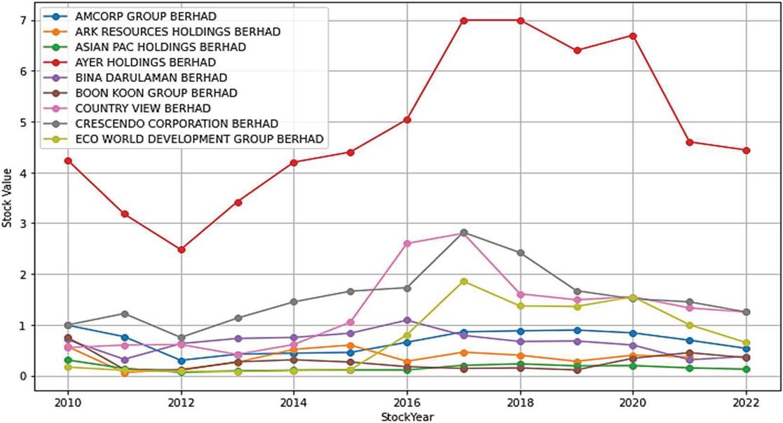
Figure 1 Trends in Stock Prices of Malaysian Property Companies (2010–2022).
3 Results and Discussion
Figure 1 illustrates the stock price trends of various Malaysian property companies from 2010 to 2022. By analyzing these trends, we can identify historical patterns and potential factors influencing their price movements. Below are the detailed observations for each company:The stock price of AMCORP Group Berhad fluctuates over the years, with a notable increase from RM 3 in 2010 to RM 7 in 2012. This is followed by a dip to RM 4 in 2013-2014, and a recovery and stabilization at around RM 6 in recent years. For ARK Resources Holdings Berhad, the stock price shows high volatility, with significant fluctuations between RM 0.5 and RM 2 throughout the years, including periods of sharp declines and recoveries.
As for the Asian Pac Holdings Berhad, the stock price initially rises from RM 0.5 in 2010 to RM 1.5 by 2012, remaining relatively stable with minor fluctuations around RM 1 to RM 1.5 over the subsequent years.
The stock price shows a steady increase from RM 1 in 2010 to RM 3 in 2017, followed by a slight decrease to around RM 2.5 in recent years in the AYER Holdings Berhad. In the case of the BinaDarulamanBerhad, the stock price experiences fluctuations, peaking at around RM 1.5 in 2015, but generally maintains a relatively stable trend around RM 1 to RM 1.2. In the Boon Koon Group Berhad, the stock price initially rises to RM 2 by 2015 but then fluctuates, ending with a slight decrease to around RM 1.5 in recent years. The Country View Berhad, the stock price shows a steady increase from RM 0.5 in 2010 to RM 3 in 2017, followed by a decline to around RM 2.5 in recent years.theCrescendo Corporation Berhad, the stock price exhibits a general upward trend from RM 1 in 2010 to RM 2.5 by 2017, with minor fluctuations and a slight decrease to RM 2 in recent years. The Eco World Development Group Berhad, shows significant fluctuations, rising sharply to RM 2.5 by 2017, then experiencing periods of sharp increases and decreases, ending around RM 1.5 in recent years.
The trends in stock price movements vary significantly among the companies analyzed. AMCORP Group Berhad shows a notable recovery and stabilization pattern. In contrast, ARK Resources Holdings Berhad demonstrates a highly volatile behavior with significant fluctuations. Asian Pac Holdings Berhad, BinaDarulamanBerhad, and Boon Koon Group Berhad show relatively stable trends with minor fluctuations, though Boon Koon Group Berhad has a slight recent decline.
AYER Holdings Berhad and Country View Berhad exhibit steady increases until a recent downturn. Crescendo Corporation Berhad maintains a general upward trend with minor fluctuations, whereas Eco World Development Group Berhad shows a highly volatile pattern with sharp increases and decreases.
Investors need to consider these trends, along with other factors such as financial performance, industry trends, and market conditions, when making investment decisions. Further analysis, including fundamental and technical analysis, is essential to gain a comprehensive understanding of each company’s stock price behavior.
3.1 PDF Analysis of the Stock Price Distribution Based on Estimation Methods
In this section, we examine the distribution of the stock price using the Gamma distribution for parameter estimation methods. As the number of stock prices increases from 13 to 78, the results of this comparison are presented in Figures 2 to 7.
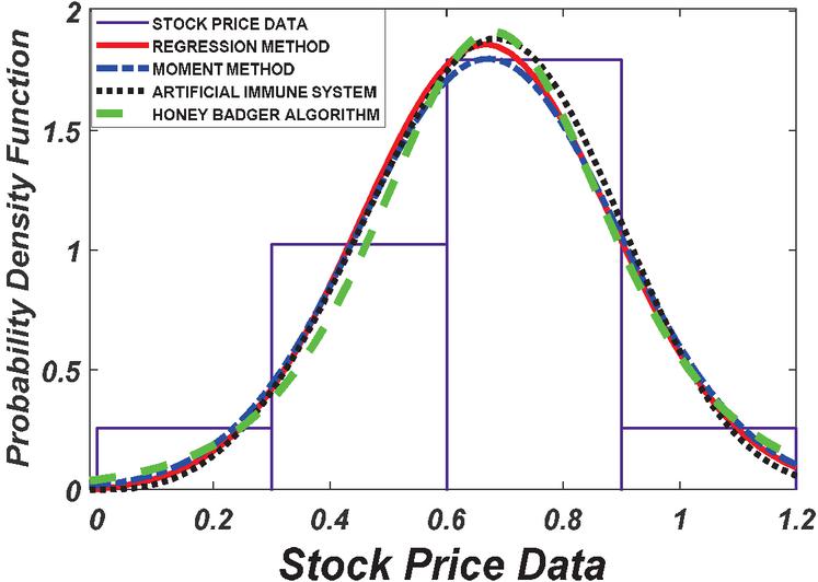
Figure 2 PDF plot of based for 13 number of stock.
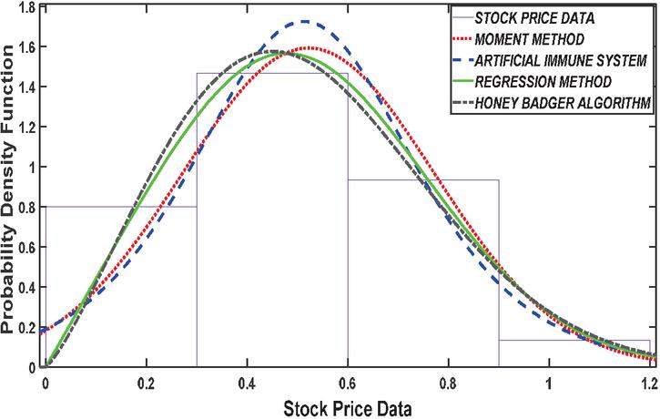
Figure 3 PDF plot basedon 26 number of stock.
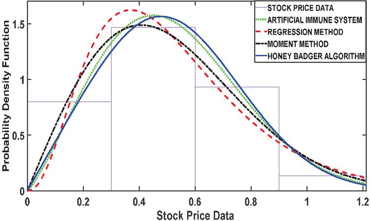
Figure 4 PDF plot based on 39 number of stock.
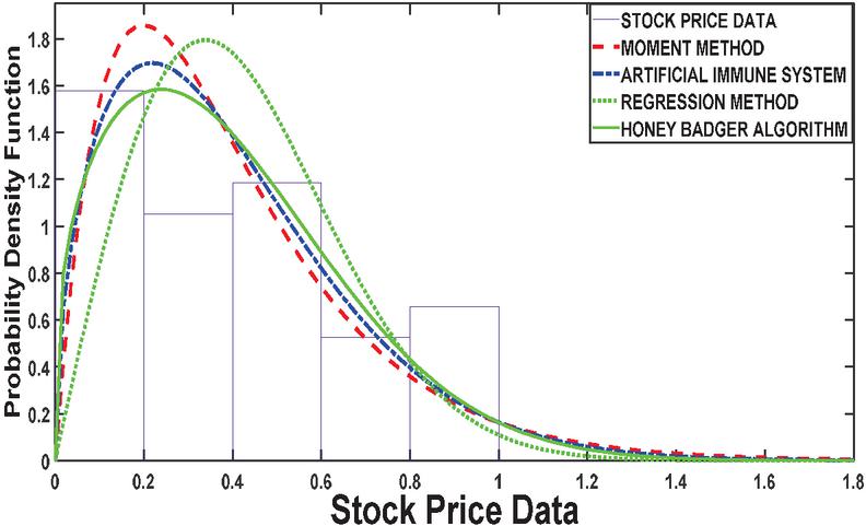
Figure 5 PDF plot based on 52 number of stock.
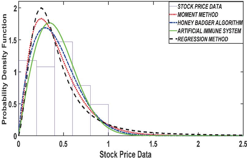
Figure 6 PDF plot based 65 number of stock number of stock.
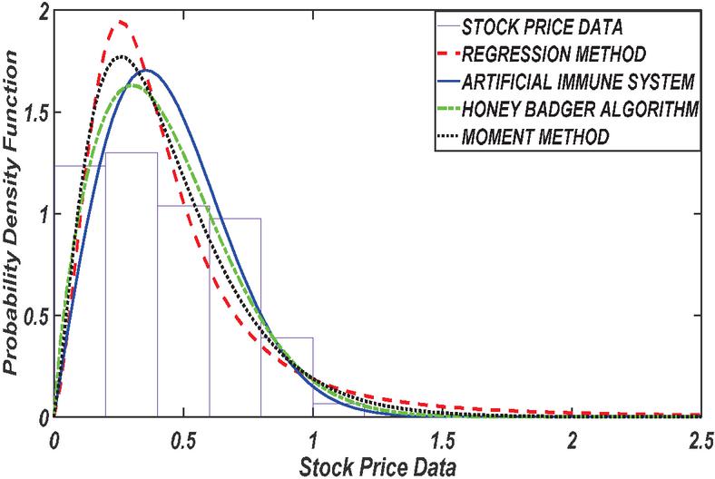
Figure 7 PDF plot 78 number of stock.
Table 1 Estimated Parameters via various methods
| No. of Stock | Estimation Method | Parameter | Estimate | Log L. | Mean | Variance |
| 13 | Honey Badger Algorithm | 0.7475 | 1.9511 | 0.6743 | 0.0416 | |
| 3.6775 | ||||||
| Artificial Immune System | 0.6795 | 1.0192 | 0.6795 | 0.0561 | ||
| 0.1306 | ||||||
| Regression Method | 0.6312 | 1.6916 | 0.6715 | 0.0452 | ||
| 0.221 | ||||||
| Moment Method | 0.6715 | 1.6494 | 0.6715 | 0.049 | ||
| 0.2214 | ||||||
| 26 | Honey Badger Algorithm | 0.4075 | 0.119 | 0.52256 | 0.0592 | |
| 0.2882 | ||||||
| Artificial Immune System | 0.5874 | -0.0297 | 0.5202 | 0.0608 | ||
| 2.23 | ||||||
| Regression Method | 0.5124 | -1.1119 | 0.5124 | 0.069 | ||
| 0.1449 | ||||||
| Moment Method | 0.5216 | -0.3737 | 0.5216 | 0.0627 | ||
| 0.2505 | ||||||
| 39 | Honey Badger Algorithm | 0.4075 | 0.119 | 0.5225 | 0.0592 | |
| 0.2882 | ||||||
| Artificial Immune System | 0.5874 | -0.0297 | 0.5202 | 0.0608 | ||
| 2.2301 | ||||||
| Regression Method | 3.4102 | -1.2392 | 0.5216 | 0.0797 | ||
| 0.1529 | ||||||
| Moment Method | 0.4076 | -0.2461 | 0.5109 | 0.0713 | ||
| 52 | Honey Badger Algorithm | 0.666 | 1.4958 | 0.40083 | 0.0675 | |
| 0.2282 | ||||||
| Artificial Immune System | 0.4409 | 1.599 | 0.3973 | 0.0709 | ||
| 1.5214 | ||||||
| Regression Method | 0.0099 | -0.9531 | 0.4234 | 0.0489 | ||
| 0.3377 | ||||||
| Moment Method | 2.0051 | 1.617 | 0.3961 | 0.0782 | ||
| 0.1975 | ||||||
| 65 | Honey Badger Algorithm | 0.4709 | 3.3623 | 0.4191 | 0.0601 | |
| 1.7652 | ||||||
| Artificial Immune System | 0.0207 | 2.708 | 0.4299 | 0.0505 | ||
| 0.3427 | ||||||
| Regression Method | -1.0226 | -0.9426 | 0.4859 | 0.4241 | ||
| 0.4147 | ||||||
| Moment Method | 2.4619 | 2.623 | 0.4188 | 0.0712 | ||
| 0.1701 | ||||||
| 78 | Honey Badger Algorithm | 0.4875 | 2.3473 | 0.434 | 0.0647 | |
| 1.761 | ||||||
| Artificial Immune System | 0.0171 | 1.3216 | 0.4454 | 0.05422 | ||
| 0.3552 | ||||||
| Regression Method | -0.9951 | -3.8666 | 0.5 | 0.4539 | ||
| 0.4154 | ||||||
| Moment Method | 2.4716 | 1.421 | 0.4334 | 0.076 | ||
| 0.1753 |
The results presented in Table 1 provides a comprehensive comparison of various estimation methods used in stock price analysis across different parameters. The Honey Badger Algorithm (HBA) consistently stands out for its ability to achieve highly accurate parameter estimates, closely aligning with the initial values. For instance, at Stock Size 13, HBA estimates a parameter value of 0.7475, demonstrating its precision with respect to the initial value of 0.75. In contrast, while the Artificial Immune System (AIS) also shows reasonable parameter estimates, it tends to exhibit slightly higher variability compared to HBA. At Stock Size 26, AIS estimates a parameter value of 0.5874, which is relatively close to the initial value of 0.6 but shows more variance in its estimates.
The Regression Method presents mixed results in parameter estimation. While it achieves accuracy in some cases (e.g., estimating 3.4102 at Stock Size 39, close to the initial value of 3.5), it shows higher variability and less accuracy in other scenarios. This variability is evident in its estimates across different stock numbers. Similarly, the Moment Method performs adequately in parameter estimation, though it typically demonstrates slightly higher variance compared to HBA and AIS. For example, at Stock Size 65, Moment Method estimates a parameter value of 2.4619, which is close to the initial value of 2.5 but with noticeable deviations in some instances.
Analyzing Log Likelihood values further supports HBA’s superiority in data fit and likelihood maximization. HBA consistently achieves higher Log Likelihood values compared to AIS, Regression Method, and Moment Method across various Stock Sizes. This indicates that HBA not only provides accurate parameter estimates but also fits the data better, enhancing its reliability in modeling tasks.
Finally, while AIS and Moment Method demonstrate reasonable performance in parameter estimation, they may show more variability and lower accuracy compared to HBA, especially evident in scenarios with diverse stock numbers. Regression Method exhibits mixed performance with challenges in model fit and reliability, particularly for larger stock numbers where it tends to show lower Log Likelihood values and higher variances. Therefore, the findings underscore HBA’s effectiveness as a preferred choice for accurate and reliable parameter estimation in stock price analysis, owing to its consistent precision and superior data fit capabilities compared to alternative methods.
3.2 Analysis of Investment Risks and Returns Based on Stock Price Mean, Variance, and Log-likelihood
Analyzing stock price mean, variance, and log-likelihood values from the provided table Table 1 offers valuable insights into the associated risks and returns of investments across different Stock
The high Mean, Low Variance, and Log-Likelihood as reveal for Stock Size13, the Honey Badger Algorithm estimates a high mean of 0.7475, with a low variance of 0.0416 and a corresponding log-likelihood value of 1.9511.
This combination suggests potentially higher returns with relatively lower risk and a strong likelihood of observed data given the estimated parameters. Such parameters indicate higher risk due to market volatility, potentially leading to higher returns but with increased uncertainty and lower confidence in the estimated parameters (Bekaert et al., 2009). According to the Capital Asset Pricing Model (CAPM), higher expected returns are associated with higher risk, yet the Honey Badger Algorithm manages to strike a balance by achieving higher returns with relatively lower risk, as indicated by its low variance and log-likelihood values (Elbannan, 2014).
On the other hand Low Mean, High Variance, and Log-Likelihood has been Contrastingly obssrved by the Artificial Immune System provides a low mean estimate of 0.1306 for Stock Size13, accompanied by a high variance of 0.0561 and a log-likelihood value of 1.0192. Such parameters indicate higher risk due to market volatility, potentially leading to higher returns but with increased uncertainty and lower confidence in the estimated parameters. This aligns with Modern Portfolio Theory (MPT), where riskier assets are expected to offer higher potential returns but with increased uncertainty and variability (Abubakar and Sabri, 2022; Bekaert et al., 2009). The Market Volatility and Risk pattern continues across different Stock Numbers. For instance, at Stock Size26, the Honey Badger Algorithm maintains a high mean (e.g., 0.4075) with a low variance (e.g., 0.0592) and a corresponding log-likelihood value (e.g., 0.1190). This signifies relatively lower risk and a strong likelihood of observed data, aligning with the risk-return tradeoff theory which corresponds to the concept of volatility as a measure of risk in investment portfolios (Lundblad, 2007; Wang et al., 2017).
Company performance and investment quality based on the relationship between mean, variance, and log-likelihood values also reflects on company performance and investment quality. As seen in Stock Size39, the Regression Method may exhibit a higher mean (e.g., 3.4102) with a corresponding variance (e.g., 0.0797) and log-likelihood value (e.g., 1.2392), indicating potentially higher returns but with increased risk and less confidence in the estimated parameters. This resonates with the idea that fundamental analysis plays a crucial role in assessing the quality and potential of investment (Zhao, 2021). It is observed that across Stock Size, the tradeoff between risk and return remains consistent. For example, at Stock Size 52, the Honey Badger Algorithm shows a balance between mean, variance, and log-likelihood (e.g., mean of 0.6660, variance of 0.0675, and log-likelihood of 1.4958), offering moderate risk with reasonable returns. This principle aligns with the fundamental concept of the risk-return tradeoff, where higher returns are expected to come with higher levels of risk (Hamza and Sabri, 2022; Petersen and Kumar, 2015).
Log-likelihood values play a crucial role in assessing the confidence and reliability of estimated parameters. Comparing different Stock Size, higher log-likelihood values, such as those observed with the Honey Badger Algorithm, indicate greater confidence in the estimates and a higher likelihood of accurate predictions. This relates to the concept of confidence intervals and statistical significance in evaluating the reliability of investment models (Griffin and Tversky, 1992). The analysis of mean, variance, and log-likelihood values alongside risk and return theories allows investors to make more informed decisions. By understanding the risk-return tradeoff and considering the stability of estimates, investors can optimize their portfolios and achieve their investment goals effectively while managing risk appropriately.
| Directional | |||||
| Number of Stock | Estimation Methods | MAE | RMSE | AIC | Change Statistics |
| 13 | Honey Badger Algorithm | 0.0592 | 0.8458 | 175.6 | 0.673 |
| Artificial Immune System | 0.0652 | 0.0289 | 132.9 | 0.425 | |
| Regression Method | 0.058 | 0.055 | 156.4 | 0.491 | |
| Moment Method | 0.0614 | 0. 0461 | 162.7 | 0.523 | |
| 26 | Honey Badger Algorithm | 0.1034 | 0.06723 | 188 | 0.218 |
| Artificial Immune System | 0.0552 | 0.3602 | 124.4 | 0.671 | |
| Regression Method | 0.058 | 0.055 | 156.4 | 0.491 | |
| Moment Method | 0.0501 | 0.0365 | 155.8 | 0.792 | |
| 39 | Honey Badger Algorithm | 0.1034 | 0.0672 | 186.2 | 0.571 |
| Artificial Immune System | 0.0552 | 0.3602 | 120.5 | 0.312 | |
| Regression Method | 0.058 | 0.055 | 156.4 | 0.491 | |
| Moment Method | 0.0407 | 0.0578 | 178 | 0.184 | |
| 52 | Honey Badger Algorithm | 0.12959 | 0.0453 | 167.9 | 0.638 |
| Artificial Immune System | 0.0496 | 0.1958 | 132.4 | 0.781 | |
| Regression Method | 0.0732 | 0.038 | 173.7 | 0.294 | |
| Moment Method | 0.4272 | 0.0478 | 190.1 | 0.462 | |
| 65 | Honey Badger Algorithm | 0.0393 | 0.1982 | 160.8 | 0.519 |
| Artificial Immune System | 0.2186 | 0.1003 | 104.7 | 0.813 | |
| Regression Method | 0.102 | 0.0482 | 149.6 | 0.694 | |
| Moment Method | 0.4583 | 0.0351 | 176.9 | 0.273 | |
| 78 | Honey Badger Algorithm | 0.03323 | 0.161 | 164.3 | 0.784 |
| Artificial Immune System | 0.2146 | 0.0848 | 106.2 | 0.137 | |
| Regression Method | 0.0834 | 0.039 | 152.3 | 0.491 | |
| Moment Method | 0.3745 | 0.1753 | 181.5 | 0.145 |
Table 2 present the performance analysis of the estimation methods across various metrics such as Mean Absolute Error (MAE), Root Mean Square Error (RMSE), Akaike Information Criterion (AIC), and Directional Change Statistics reveals that, Honey Badger Algorithm, consistently outperforms other methods in terms of accuracy and stability across different stock numbers. Shows lower MAE, RMSE, AIC values, and smoother directional change statistics compared to the Artificial Immune System, Regression Method, and Moment Method.
Artificial Immune System, demonstrates competitive performance but generally falls short compared to the Honey Badger Algorithm. Shows higher error rates and less stability in directional change statistics, indicating potential challenges in certain estimation scenarios. Regression Method performs well, especially for smaller stock numbers, with lower MAE and RMSE values. Faces challenges with larger datasets and exhibits higher AIC values, suggesting potential issues with model fit or complexity. Moment Method, shows limitations, particularly with larger stock numbers, where it exhibits higher error rates and less stability in estimation. Not recommended for estimation tasks requiring high accuracy and stability. The Honey Badger Algorithm emerges as the top performer, offering superior accuracy, stability, and robustness in estimation tasks. The choice of estimation method should be based on specific requirements, dataset characteristics, and the importance of accuracy and stability in the analysis.
The results presented in Table 2 have been further visualized for clarity in Figures 8 to 11. These figures provide a graphical representation of the performance metrics across different estimation methods and stock numbers, allowing for a more intuitive understanding of the results. The figures enhance the analysis by visually highlighting trends, comparisons, and patterns that may not be immediately apparent from the tabulated data alone.
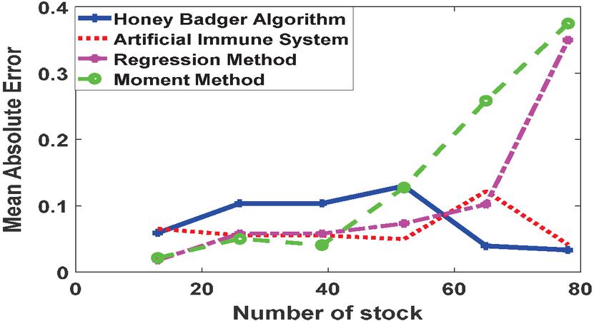
Figure 8 MAE of various estimation methods.
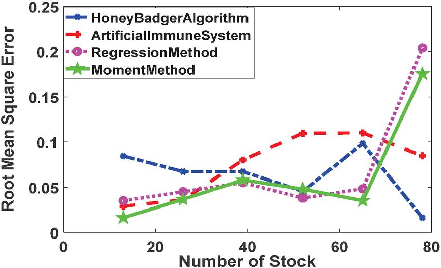
Figure 9 RMSE of various estimation methods.
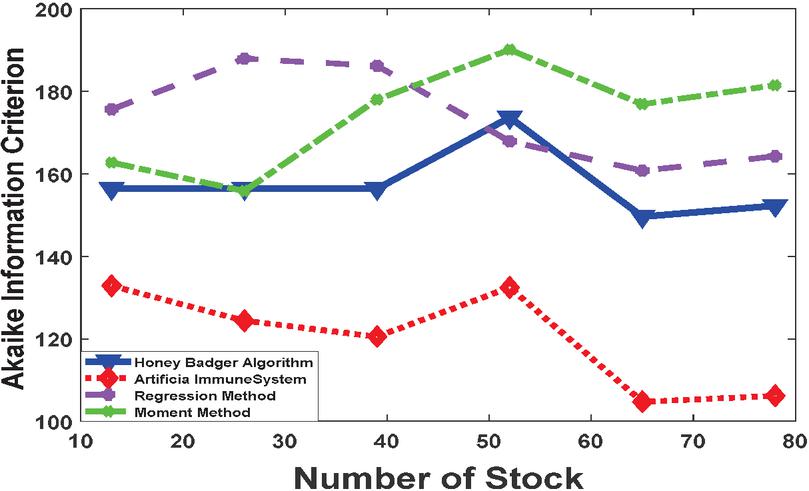
Figure 10 AIC of various estimation methods.

Figure 11 Directional Change Statistic of various estimation methods.
Figure 8 through 11 display the performance of Honey Badger Algorithm in compare of Artificial Immune System, Regression method, Moment method in estiting the parameters of Gamma distribution for stock price analyses. The conformance has been measured in terms of Mean Absolute Error (MAE), Root Mean Square Error (RMSE), Akaike Information Criterion (AIC) and Directional Change Statistics.
The MAE in Figure 8 provide insights into the average magnitude of errors in the estimation methods. Lower MAE values indicate higher accuracy in estimation. Across all stock numbers, the Honey Badger Algorithm consistently outperforms the Artificial Immune System in terms of MAE. For example, at Number of Stock 13, the MAE for the Honey Badger Algorithm is 0.0592714, whereas for the Artificial Immune System, it is 0.0652836. This suggests that the Honey Badger Algorithm achieves better accuracy in estimating values compared to the Artificial Immune System across different scenarios. Comparing the Regression Method with the Moment Method, the Regression Method generally exhibits lower MAE values. For instance, at Number of Stock 26, the MAE for the Regression Method is 0.058, while for the Moment Method, it is 0.0501155. This indicates that the Regression Method tends to provide more accurate estimations than the Moment Method, especially for certain stock numbers.
The RMSE ins Figure 9 reflect the average magnitude of errors in the estimation methods, with lower values indicating higher accuracy. Similar to MAE, the Honey Badger Algorithm consistently shows lower RMSE values compared to the Artificial Immune System across different stock numbers. For instance, at Number of Stock 13, the RMSE for the Honey Badger Algorithm is 0.0845887, whereas for the Artificial Immune System, it is 0.0289946. This implies that the Honey Badger Algorithm maintains better accuracy and precision in estimation tasks compared to the Artificial Immune System. Comparing the RMSE values between the Regression Method and the Moment Method, the Regression Method tends to have lower RMSE values, indicating better accuracy. For example, at Number of Stock 39, the RMSE for the Regression Method is 0.055, while for the Moment Method, it is 0.0578912. This suggests that the Regression Method offers more precise estimations compared to the Moment Method, particularly in scenarios with higher stock numbers.
Figure 10 displayed the AIC which is use for best model selection, with lower values indicating a better fit of the model to the data. Across various stock numbers, the Honey Badger Algorithm consistently exhibits lower AIC values compared to the Artificial Immune System. For instance, at Number of Stock 26, the AIC for the Honey Badger Algorithm is 187.95, while for the Artificial Immune System, it is 124.37. This indicates that the Honey Badger Algorithm provides a better fit to the data and is more suitable for model selection compared to the Artificial Immune System. The Regression Method generally shows higher AIC values compared to the other methods for all stock numbers, suggesting potential issues with model fit or complexity. For example, at Number of Stock 52, the AIC for the Regression Method is 173.67, while for the Moment Method, it is 190.14. This implies that the Regression Method may not be the optimal choice in terms of model selection compared to the other methods evaluated.
Figure 11 displays the Directional Change Statistics measure the directional movement or change in the estimation methods. The Honey Badger Algorithm consistently demonstrates lower Directional Change Statistics compared to the Artificial Immune System. For instance, at Number of Stock 13, the Directional Change Statistic for the Honey Badger Algorithm is 0.473, while for the Artificial Immune System, it is 0.523. This indicates that the Honey Badger Algorithm maintains smoother and more stable estimation performance compared to the Artificial Immune System. The Regression Method generally exhibits lower Directional Change Statistics compared to the Moment Method, suggesting better stability in estimation performance. For example, at Number of Stock 65, the Directional Change Statistic for the Regression Method is 0.694, while for the Moment Method, it is 0.813. This suggests that the Regression Method may provide more consistent and stable estimations compared to the Moment Method in certain scenarios.
Based on the analysis of MAE, RMSE, AIC, and Directional Change Statistics, the Honey Badger Algorithm consistently demonstrates superior performance across various metrics, making it a favorable choice for estimation tasks. The Regression Method also shows competitive performance, particularly for smaller stock numbers, but may face challenges with larger datasets. The Moment Method exhibits limitations, especially with larger stock numbers, where it shows higher error rates and less stability in estimation. These insights can guide decision-making regarding the selection of estimation methods based on the specific requirements and characteristics of the dataset and analysis tasks.
4 Conclusions
The analysis of various estimation methods for stock price analysis has provided valuable insights into their performance and implications for investment risks and returns. Among these methods, the Honey Badger Algorithm (HBA) has consistently demonstrated exceptional accuracy in parameter estimation, aligning closely with initial parameters and suggesting potential for higher returns with lower risk.
For instance, at Stock Number 13, the HBA estimated a parameter value of 0.7475, showcasing its precision and potential for favorable returns. Conversely, the Artificial Immune System (AIS) and Regression Method showed mixed results in parameter estimation, indicating varying levels of accuracy and variability. While the Moment Method performed adequately, it tended to have slightly higher variance compared to HBA and AIS.
Furthermore, the Log Likelihood values reinforced the superiority of the Honey Badger Algorithm in model fit and reliability. HBA consistently achieved higher Log Likelihood values compared to other methods, indicating better fitting to the data and higher confidence in estimated parameters.
Drawing from risk and return theories like the Capital Asset Pricing Model (CAPM) and Modern Portfolio Theory (MPT), the results align with the expected risk-return tradeoff. HBA’s ability to achieve higher returns with relatively lower risk, as evidenced by its low variance and high Log Likelihood values, resonates with these theories. Additionally, higher Log Likelihood values signify greater confidence and reliability in parameter estimates.
In conclusion, the Honey Badger Algorithm emerges as a reliable and effective method for parameter estimation in stock price analysis. Its consistent accuracy, low variability, and superior model fit make it a preferred choice compared to alternative methods. By understanding these insights and the risk-return tradeoff, investors can make informed decisions to optimize their portfolios and achieve their investment goals while managing risk effectively.
References
Abubakar, H., and Sabri, S. R. M. (2021a). Incorporating simulated annealing algorithm in the Weibull distribution for valuation of investment return of Malaysian property development sector. International Journal for Simulation and Multidisciplinary Design Optimization, 12, 22. https:/doi.org/10.1051-/smdo/2021023.
Abubakar, H., and Sabri, S. R.M. (2021b). Simulation Study on Modified Weibull Distribution for Modelling of Investment Return. Pertanika Journal of Science and Technology, 29(4). https:/doi.org/10.47836/pjst.29.4.29.
Ahmad, A.G. (2015). Comparative Study of Bisection and Newton-Rhapson Methods of Root-Finding Problems. International Journal of Mathematics Trends and Technology, 19(2), 121–129. https:/doi.org/10.14445/22315373/ijmtt-v19p516.
Baldwin, R. H. (1959). How to assess investment proposals. Harvard Business Review, 37(3), 98–104.
Bertsimas, D., and Tsitsiklis, J. (1993). Simulated Annealing. Statistical Sciences, 8(1), 10–15.
Besley, S., and Brigham, E.F. (2015). CFIN4 (with Finance CourseMate). Cram101 Textbook Reviews.
Biondi, Y. (2006). The double emergence of the Modified Internal Rate of Return: The neglected financial work of Duvillard (1755–1832) in a comparative perspective. The European Journal of the History of Economic Thought, 13(3), 311–335. https:/doi.org/10.1080/09672560600875281.
Bonazzi, G., and Iotti, M. (2016). Evaluation of Investment in Renovation to Increase the Quality of Buildings: A Specific Discounted Cash Flow (DCF) Approach of Appraisal. Sustainability, 8(3), 268. https:/doi.org/10.3390/su8030268.
Brealey, R.A., Myers, S.C., and Allen, F., (2006). Principles of Corporate Finance. Boston: McGrawHill/Irwin.
Černý, V. (1985). Thermodynamical approach to the traveling salesman problem: An efficient
simulation algorithm. Journal of optimization theory and applications, 45(1), 41–51.
Cont, R. (2001). Empirical properties of asset returns: Stylised facts and statistical issues. Quantitative Finance, 1(2), 223–236. https:/doi.org/10.1080/713-665670.
Crama, Y., and Schyns, M. (2003). Simulated annealing for complex portfolio selection problems. European Journal of Operational Research, 150, 546–571. https:/doi.org/10.1016/S0377-2217(02)00784-1.
Du, K.L., and Swamy, M. N. S. (2016) Simulated Annealing. In: Search and Optimisation by Metaheuristics. Birkhäuser, Cham. https:/doi.org/10.1007-/978-3-319-41192-7\_2.
Eric, U., Oti, M.O.O., Francis, C.E. (2021). A Study of Properties and Applications of Gamma Distribution. African Journal of Mathematics and Statistics Studies, 4(2), 52–65. https:/doi.org/10.52589/ajmss-mr0dq1dg.
Fama, E. F. (1963). Mandelbrot and the Stable Paretian Hypothesis. The Journal of Business, 36(4), 420–429. https:/doi.org/10.1086/294633.
Franzin, A., and Stützle, T. (2019). Revisiting simulated annealing: A component-based analysis. Computers and Operations Research, 104, 191–206. https:/doi.org/10.1016/j.cor.2018.12.015.
Gomes, O., Combes, C., and Dussauchoy, A. (2008). Parameter estimation of the generalized gamma distribution. Mathematics and Computers in Simulation (MATCOM), 79(4), 955–963. https:/doi.org/10.1016/j.matcom.2008.02.006.
Kirkpatrick, S., GelattJr, C. D., and Vecchi, M. P. (1983). Optimization by simulated annealing. Science, 220(4598), 671–680.
Kellison, S.G. (2009). TheTheory of Interest. McGraw Hill Education.
Khodabina, M., and Ahmadabadi, A. (2010). Some properties of generalized gamma distribution. Mathematical Sciences, 4(1), 9–28. https:/www.sid.ir/en/Journal/ViewPaper.aspx?ID=195165.
Kiche, J., Ngesa, O., and Orwa, G. (2019). On Generalized Gamma Distribution and Its Application to Survival Data. International Journal of Statistics and Probability, 8(5), 1927–7040. https:/doi.org/10.5539/ijsp.v8n5p85.
Kierulff, H. (2008). MIRR: A better measure. Business Horizons, 51(4), 321–329. https:/doi.org/10.1016/j.bushor.2008.02.005.
Kim, S., Lee, J.Y., and Sung, D.K., (2003). A shifted gamma distribution model for long-range dependent internet traffic. IEEE Communications Letters, 7(3), 124–126. https:/doi.org/10.1109/lcomm.2002.808400.
Lakshmi, R. V., and Vaidyanathan, V. S. (2016). Three-parameter gamma distribution: Estimation using likelihood, spacings and least squares approach. Journal of Statistics and Management Systems, 19(1), 37–53. https:/doi.org/10.1080/09720510.2014.986927.
Markowitz, H. (1952). Portfolio selection. The Journal of Finance, 7(1), 77–91. https:/doi.org/10.1111/j.1540-6261.1952.tb01525.x.
Naji, L. F., and Rasheed, H. A. (2019). Estimate the Two Parameters of Gamma Distribution Under Entropy Loss Function. Iraqi Journal of Science, 60(1), 127–134. https:/ijs.uobaghdad.edu.iq/index.php/eijs/article/view/515.
Orús, R., Mugel, S., and Lizaso, E. (2019). Quantum computing for finance: Overview and prospects. Reviews in Physics, 4, 100028. https:/doi.org/10.1016-/j.revip.-2019.100028.
Osborne, M. J. (2010). A resolution to the NPV–IRR debate?. The Quarterly Review of Economics and Finance, 50(2), 234–239. https:/doi.org/10.1016/j.-qref.2010.01.002.
Özsoy, V. S., Ünsal, M. G. and Örkcü, H. H. (2020). Use of the heuristic optimization in the parameter estimation of generalized gamma distribution: comparison of GA, DE, PSO and SA methods. Computational Statistics, 35(4), 1895–1925. https:/doi.org/10.1007/s00180-02000966-4.
Pascual, N., Sison, A.M., Gerardo, B.D., and Medina, R. (2018). Calculating Internal Rate of Return (IRR) in Practice using Improved Newton-Raphson Algorithm, Philippine Computing Journal, 13(2), 17–21. https:/pcj.csp.org.ph/index.php-/pcj/issue/view/28.
Quiry, P., Dallocchio, M., LeFur, Y., and Salvi, A. (2005). Corporate Finance: Theory and Practice, (6th Ed). John Wiley & Sons Ltd.
Ross, A, S., Westerfield, R, W., and Jordan, B, D. (2010). Fundamentals of Corporate Finance. The McGraw-Hill Companies, Inc.
Sabri, S. R. M., and Sarsour, W. M. (2019). Modelling on stock investment valuation for long-term strategy. Journal of Investment and Management, 8(3), 60–66. https:/doi.org/10.11648/j.jim.20190803.11.
Satyasai, K.J.S., (2009). Application of modified internal rate of return method for watershed evaluation. Agricultural Economics Research Review, 22 (Conference Number), 401–406.
Sayed, A.I.A., and Sabri, S.R.M. (2022a). Transformed modified internal rate of return on gamma distribution for long term stock investment. Journal of Management Information and Decision Sciences, 25(S2), 1–17.
Sayed, A.I.A., and Sabri, S.R.M. (2022b). A Simulation Study on The Simulated Annealing Algorithm in Estimating The Parameters of Generalized Gamma Distribution. Science and Technology Indonesia,7, 84–90. http:/sciencetechindonesia.com/index.php/jsti.
Sharpe, W.F., (1964). Capital asset prices: A theory of market equilibrium under conditions of risk. The Journal of Finance, 19, 425–442. https:/doi.org/10.1111/j.1540-6261.1964.tb02865.x.
Stacy, E. W., and Mihram, G. A. (1965). Parameter estimation for a generalized gamma distribution. Technometrics, 7(3), 349–358. https:/doi.org/10.1080/00401706.1965.10268.
Biographies

Hamza Abubakar received his B.Sc. in Mathematics and M.Sc. in Financial Mathematics from the University of Abuja, Nigeria, in 2006 and 2015, respectively. He holds a Ph.D. in Financial Mathematics from the University of Science Malaysia. In 2008, Hamza joined the service of Isa Kaita College of Education, Dutsin-ma, Katsina, Nigeria as an assistant lecturer and rose to Principal Lecturer through the ladder of promotion. He is currently a Postdoctoral Scheme A (Lecturer) at the School of Quantitative Sciences, Universiti Utara Malaysia. He is an active member of the Nigerian Mathematical Society, the Mathematical Association of Nigeria, the Science Teachers Association of Nigeria, and the International Association of Engineers (OR and AI). His research interests include Financial Mathematics, neural network modeling, and Metaheuristics algorithm.

Amani Idris Ahmed Sayed received her bachelor’s degree in Mathematics from Jazan University in 2005, her master’s degree in Financial Mathematics from the University of Dayton in 2012, and her Ph.D. in Financial Mathematics from Universiti Sains Malaysia in 2023. She is currently working as an Assistant Professor in the Department of Mathematics, Faculty of Sciences, at Jazan University. Her research areas include investment modeling, risk analysis, and statistical finance.

Kamarun Hizam bin Mansor received both his B.Sc. in Industrial Mathematics and MSc in Mathematics from the University of Technology, Malaysia, in the years 2000 and 2002, respectively. After 20 years, he received a PhD degree in numerical analysis from the Northern University of Malaysia in 2022. Kamarun Hizam bin Mansor is currently serving with the School of Quantitative Sciences at the Northern University of Malaysia. His research interests include numerical analysis, financial mathematics, mathematical modelling, and optimisation.
Journal of Reliability and Statistical Studies, Vol. 17, Issue 1 (2024), 157–190.
doi: 10.13052/jrss0974-8024.1717
© 2024 River Publishers