Cost-Effectiveness Analysis of a System of Distinguishable Subsystems with Repair Preference and Weather Conditions

Lalit Kumar¹, D. Pawar^1,* and Kailash Kumar²

¹Department of Statistics, Amity Institute of Applied Sciences, Amity University Uttar Pradesh, Noida – 201313, India
²Department of Statistics, LSR College for Women, University of Delhi, New Delhi – 110024, India
E-mail: dpanwar75@yahoo.com
*Corresponding Author

Received 22 July 2024; Accepted 12 November 2024

Abstract

Cost-effectiveness analysis of a reliability model of two distinguishable electricity resources is done in this paper. Subsystem-A is taken as the primary, whereas subsystem-B is taken as the secondary source of electricity. Subsystem-A has three modes – operation, repair, and activation, and subsystem-B has four modes – operation, inspection, minor repair, and major repair. Availability of a full-time technician is considered to perform all repair and activation activities. The technician initiates the repair of subsystem-A immediately whenever required, whereas inspection is carried out for subsystem-B to identify the type of repair required. Normal and abnormal weather conditions are considered to study the impact of weather conditions on repair and activation activities. Only subsystem-A needs activation after repair, and no repair/activation is carried out in abnormal weather, while weather conditions do not affect inspection or repair activities of subsystem-B. Failure and repair rates of both the subsystems are exponentially distributed, whereas a general distribution is taken for the operation rate of subsystem-A. Various reliability components like Mean Time to System Failure (MTSF), steady-state availability, busy period of the server, and profit of the system model are evaluated using the semi-Markov process. Random values are taken to show the impact of increasing failure rate of subsystem-A and rate of change of weather condition from normal to abnormal on MTSF and the cost-benefit of the system model. Graphs are drawn for MTSF and profit of the system model, which clearly indicates that MTSF and profit of the system model are higher for a lesser rate of change in weather conditions.

Keywords: Reliability, inspection, activation, semi-markov, weather, minor repair, major repair.

1 Introduction

The implication of reliability is evident throughout the planning, design, and operation stages of varied complex systems. As modern technologies continue to advance, demand for exceptionally reliable systems has grown significantly. In view of the growing demand for highly reliable systems, many researchers, including Murari and Goyal (1983), analysed the reliability of a system with two types of repair facilities. Goel et al. (1985) discussed the stochastic behaviour of man-machine systems under different weather conditions. Goel et al. (1986) obtained the reliability of a system with preventive maintenance, inspection, and two types of repairs. Tuteja and Taneja (1991) conducted cost-benefit analysis of a two-server, two-unit warm standby system with different failure modes. Rander et al. (1992) investigated a two-unit cold standby system with two types of failures (major and minor) by considering preparation time for repair in the case of major failure. Gupta et al. (1997) analysed the reliability of a system with preventive maintenance, inspection, and two repair policies. Sehgal (2000) studied a reliability model with partial failure, accidents, and various repair types. Siwach et al. (2001) discussed a two-unit cold standby system with instructions and accidents. Taneja and Naveen (2003) conducted a comparative study of two reliability models with patience time and the non-availability of expert repairmen. Malik et al. (2004) stochastically analysed a reliability model of non-identical units with priority and different failure modes. Pawar et al. (2010 A) discussed the reliability model of an operating system with inspection and repair at different levels of damages under different weather conditions. Pawar et al. (2010 B) studied the reliability model of a system with different repair policies in different weather conditions. Pawar et al. (2013) analysed a weathering server system under a set of assumptions. Rathee et al. (2018) completed the modelling and analysis of a parallel unit system with priority to repair/replacement subject to maximum operation and repair times. Kumar et al. (2019) conducted profit analysis of a dissimilar unit system in different weather conditions. Kumar et al. (2022) analysed the cost-effectiveness of a complex system with diverse repair policies under normal weather conditions. Ram et al. (2022) analysed a stochastic model rework system. Chachra et al. (2023) explored an intuitionistic fuzzy approach to reliability assessment of multi-state systems. Ghosh et al. (2023) analysed the performance of a non-identical units system with inspection and operational priority. Various systems require some activation time and undergo activation processes after repair. For example, solar systems require some activation time before starting their intended functions after repair. Considering this aspect, in the present paper we developed a reliability model of two non-identical subsystems: A and B, under the following assumptions.

• Initially, subsystem A is operative, and subsystem B is in cold standby mode.

• Subsystem-A has three modes – operation, repair, and activation, whereas subsystem-B has four modes – operation, inspection, minor repair, and major repair.

• Normal and abnormal weather conditions are taken to see their impact on repair and activation of the subsystems.

• All-time availability of a single technician is considered with the system to perform all repair and activation activities.

• Subsystem-A undergoes repair immediately whenever required, whereas inspection is carried out for subsystem-B to identify the requirement of minor/major repair.

• Subsystem-A requires activation after repair, and no activation activity is carried out in abnormal weather while there is no impact on inspection/repair of subsystem-B.

• Failure and repair rates of both the subsystems are exponentially distributed, whereas general distribution is taken as the rate at which subsystem-A operates.

• Various reliability measures such as MTSF, steady-state availability, busy period of the server, and profit of the system model are analyzed using the semi-Markov process.

• Arbitrary values are taken to represent the outputs of the system model graphically.

The scope of the present work is in all types of industries that consume electricity. All industries are depending on the electricity supplied by power grids. The present study will help those industries that are looking at solar systems as an alternate and primary source of electricity and want to use off grid electricity resources. Electricity generation through solar systems and their maintenance also depends on weather conditions. Therefore, in this study we considered the impact of weather conditions for optimizing the cost-benefit of the system.

2 Notations

A${}_o$/A${}_r$/A${}_a$:	Subsystem-A is operative in normal mode/ failed and under repair/ repaired and under activation.
A${}_R$/A${}_{bwa}$:	Subsystem-A is under continuous repair from previous state/ waiting for activation due to abnormal weather.
B${}_o$/B${}_{cs}$:	Subsystem-B is operative in normal mode/ is in cold standby mode.
B${}_{fwi}$/B${}_{fui}$:	Subsystem-B is failed and waiting for inspection/ is under inspection.
B${}_{wr1}$/ B${}_{r1}$:	Subsystem-B is failed and waiting for minor repair/ under minor repair.
B${}_{Wr2}$/ B${}_{r2}$:	Subsystem-B is failed and waiting for major repair/ under major repair.
$\alpha$ / $\lambda$:	Failure rate of subsystem-A/ subsystem-B.
$\theta$:	Inspection rate of subsystem-B.
a/b:	Probability that the failed subsystem-B goes for minor/ major repair.
$\beta$:	Repair rate of subsystem-A.
$\delta$:	Rate of change of weather from normal to abnormal.
${\delta }_1$:	Activation rate of subsystem-A.
G${}_1$($\cdot$)/G${}_2$($\cdot$):	c.d.f. of minor/ major repair rates of subsystem-B.
H ($\cdot$):	c.d.f. of activation rate of subsystem-A.
${\mathrm{q}}_{\mathrm{ij}}$:	Transition probability by which system transits from state ${\mathrm{S}}_{\mathrm{i}}$ to ${\mathrm{S}}_{\mathrm{j}}$ on or before time ‘t’.
${\psi }_{\mathrm{i}}$:	Mean sojourn time in the state ‘i’ is the probable waiting time of the system in the i${}^{th}$ state before moving to another state. If sojourn time in i${}^{th}$ state is ${\mathrm{T}}_{\mathrm{i}}$ then ${\psi }_{\mathrm{i}}=\int \mathrm{P}({\mathrm{T}}_{\mathrm{i}}>\mathrm{t})\mathrm{dt}$.
${\mathrm{z}}_{\mathrm{i}}$:	Probability that the system stays in state S${}_i$ up to time ‘t’.
${\mathrm{m}}_{\mathrm{ij}}$:	System’s mean sojourn time in the i${}^{th}$ state when the system is to transit to the j${}^{th}$ regenerative state i.e., ${\mathrm{m}}_{\mathrm{ij}}=\int {\mathrm{tq}}_{\mathrm{ij}}(\mathrm{t})\mathrm{dt}$.
*/**:	Symbol of Laplace Stieltjes Transformation/ Laplace Transformation.
©/${}^{\prime }$(desh):	Symbols for Laplace Convolution/ derivative of the function.
${\mathrm{K}}_0$:	Revenue per unit up-time when system is operative.
${\mathrm{K}}_1$:	Repairing cost per unit of time for subsystem-A.
${\mathrm{K}}_2$:	Cost per unit of time when subsystem-A is under activation.
${\mathrm{K}}_3$:	Cost per unit of time when subsystem-B is under inspection.
${\mathrm{K}}_4$:	Repairing cost per unit of time for subsystem-B.
${\mathrm{K}}_5$:	Fixed amount paid to the server per unit time.

The possible transition states with their transition rates are shown in Figure 1.

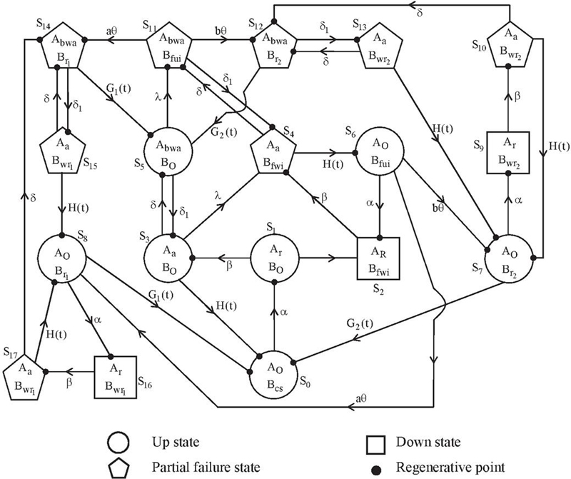
Figure 1 Transition diagram.

3 Transition Probabilities and Mean Sojourn Times

The probabilities of steady-state transitions are calculated as follows:

$${\mathrm{p}}_{\mathrm{ij}}=\underset{\mathrm{t}\to \mathrm{\infty }}{lim}{\mathrm{Q}}_{\mathrm{ij}}(\mathrm{t});{\mathrm{p}}_{\mathrm{ij}}^{(\mathrm{k})}(\mathrm{t})=\underset{\mathrm{t}\to \mathrm{\infty }}{lim}{\mathrm{Q}}_{\mathrm{ij}}^{(\mathrm{k})}(\mathrm{t})$$

Therefore,

$${\mathrm{p}}_{01}={\mathrm{p}}_{24}={\mathrm{p}}_{9,10}={\mathrm{p}}_{16,17}=1;{\mathrm{p}}_{13}=\frac{\beta }{\beta +\lambda };{\mathrm{p}}_{14}^{(2)}=1-\frac{\beta }{\beta +\lambda };$$

$${\mathrm{p}}_{30}=\tilde{\mathrm{H}}(\delta +\lambda );{\mathrm{p}}_{35}=\frac{\delta [1-\tilde{\mathrm{H}}(\delta +\lambda )]}{\delta +\lambda };$$

$${\mathrm{p}}_{3,11}^{(4)}=[1-\tilde{\mathrm{H}}(\delta )]-\frac{\delta [1-\tilde{\mathrm{H}}(\delta +\lambda )]}{\delta +\lambda };{\mathrm{p}}_{36}^{(4)}=\tilde{\mathrm{H}}(\delta )-\tilde{\mathrm{H}}(\delta +\lambda );$$

$${\mathrm{p}}_{46}={\mathrm{p}}_{10,7}={\mathrm{p}}_{13,7}={\mathrm{p}}_{15,18}={\mathrm{p}}_{17,8}=\tilde{\mathrm{H}}(\delta );$$

$${\mathrm{p}}_{4,11}={\mathrm{p}}_{10,12}={\mathrm{p}}_{13,12}={\mathrm{p}}_{15,14}={\mathrm{p}}_{17,14}=1-\tilde{\mathrm{H}}(\delta );{\mathrm{p}}_{53}=\frac{{\delta }_1}{{\delta }_1+\lambda };$$

$${\mathrm{p}}_{5,11}=\frac{\lambda }{{\delta }_1+\lambda };{\mathrm{p}}_{62}=\frac{\alpha }{\alpha +\theta };{\mathrm{p}}_{67}=\frac{b\theta }{\alpha +\theta };{\mathrm{p}}_{68}=\frac{\mathrm{a}\theta }{\alpha +\theta };$$

$${\mathrm{p}}_{70}={\tilde{\mathrm{G}}}_2(\alpha );{\mathrm{p}}_{79}=1-{\tilde{\mathrm{G}}}_2(\alpha );{\mathrm{p}}_{80}={\tilde{\mathrm{G}}}_1(\alpha );{\mathrm{p}}_{8,16}=1-{\tilde{\mathrm{G}}}_1(\alpha );$$

$${\mathrm{p}}_{11,4}=\frac{{\delta }_1}{{\delta }_1+\theta };{\mathrm{p}}_{11,12}=\frac{\mathrm{b}\theta }{{\delta }_1+\theta };{\mathrm{p}}_{11,14}=\frac{\mathrm{a}\theta }{{\delta }_1+\theta };{\mathrm{p}}_{12,5}={\tilde{\mathrm{G}}}_2({\delta }_1);$$

$${\mathrm{p}}_{12,13}=1-{\tilde{\mathrm{G}}}_2({\delta }_1);{\mathrm{p}}_{14,5}={\tilde{\mathrm{G}}}_1({\delta }_1);{\mathrm{p}}_{14,15}=1-{\tilde{\mathrm{G}}}_1({\delta }_1)$$

We observe that the following relations hold true:

${\mathrm{p}}_{01}$	$={\mathrm{p}}_{13}+{\mathrm{p}}_{14}^{(2)}={\mathrm{p}}_{24}={\mathrm{p}}_{30}+{\mathrm{p}}_{35}+{\mathrm{p}}_{3,11}^{(4)}+{\mathrm{p}}_{36}^{(4)}={\mathrm{p}}_{46}+{\mathrm{p}}_{4,11}$
	$={\mathrm{p}}_{53}+{\mathrm{p}}_{5,11}={\mathrm{p}}_{62}+{\mathrm{p}}_{67}+{\mathrm{p}}_{68}={\mathrm{p}}_{70}+{\mathrm{p}}_{79}={\mathrm{p}}_{80}+{\mathrm{p}}_{8,16}$
	$={\mathrm{p}}_{9,10}={\mathrm{p}}_{10,7}+{\mathrm{p}}_{10,12}={\mathrm{p}}_{11,4}+{\mathrm{p}}_{11,12}+{\mathrm{p}}_{11,14}={\mathrm{p}}_{12,5}+{\mathrm{p}}_{12,13}$
	$={\mathrm{p}}_{13,7}+{\mathrm{p}}_{13,12}={\mathrm{p}}_{14,5}+{\mathrm{p}}_{14,15}={\mathrm{p}}_{15,8}+{\mathrm{p}}_{15,14}$
	$={\mathrm{p}}_{16,17}={\mathrm{p}}_{17,8}+{\mathrm{p}}_{17,14}=1$

3.1 Mean Sojourn Time $({\mathit{\psi }}_{\mathbf{i}})$ in State ${\mathbf{S}}_{\mathbf{i}}$ are

$${\psi }_0=\frac{1}{\alpha };{\psi }_1=\frac{1}{\beta +\lambda };{\psi }_2={\psi }_9={\psi }_{16}=\frac{1}{\beta };$$

$${\psi }_3=\int {\mathrm{e}}^{-(\delta +\lambda )\mathrm{t}}\overline{\mathrm{H}}(\mathrm{t})\mathrm{dt};$$

$${\psi }_4={\psi }_{10}={\psi }_{13}={\psi }_{15}={\psi }_{17}=\int {\mathrm{e}}^{-\delta \mathrm{t}}\overline{\mathrm{H}}(\mathrm{t})\mathrm{dt};$$

$${\psi }_5=\frac{1}{{\delta }_1+\lambda };{\psi }_6=\frac{1}{\alpha +\theta };{\psi }_7=\int {\mathrm{e}}^{-\alpha \mathrm{t}}{\overline{\mathrm{G}}}_2(\mathrm{t})\mathrm{dt};$$

$${\psi }_8=\int {\mathrm{e}}^{-\alpha \mathrm{t}}{\overline{\mathrm{G}}}_1(\mathrm{t})\mathrm{dt};{\psi }_{11}=\frac{1}{{\delta }_1+\theta };{\psi }_{12}=\int {\mathrm{e}}^{-{\delta }_1\mathrm{t}}{\overline{\mathrm{G}}}_2(\mathrm{t})\mathrm{dt};$$

$${\psi }_{14}=\int {\mathrm{e}}^{-{\delta }_1\mathrm{t}}{\overline{\mathrm{G}}}_1(\mathrm{t})\mathrm{dt}$$

Now, we define ${\mathrm{m}}_{\mathrm{ij}}$ as

$${\mathrm{m}}_{\mathrm{ij}}=\int \mathrm{t}d{\theta }_{\mathrm{ij}}(\mathrm{t})=\int \mathrm{t}{\mathrm{q}}_{\mathrm{ij}}(\mathrm{t})\mathrm{dt}$$

So, we have

$${\mathrm{m}}_{01}=\int \mathrm{t}\alpha {\mathrm{e}}^{-\alpha \mathrm{t}}\mathrm{dt}=\alpha \int {\mathrm{t}}^{2-1}{\mathrm{e}}^{-\alpha \mathrm{t}}\mathrm{dt}=\alpha \frac{\mathrm{\Gamma }(2)}{{\alpha }^2}=\frac{1}{\alpha }$$

Similarly,

$${\mathrm{m}}_{13}=\frac{\beta }{{(\beta +\lambda )}^2};{\mathrm{m}}_{24}={\mathrm{m}}_{9,10}={\mathrm{m}}_{16,17}=\frac{1}{\beta };$$

$${\mathrm{m}}_{30}=\int \mathrm{t}{\mathrm{e}}^{-(\delta +\lambda )\mathrm{t}}\mathrm{dH}(\mathrm{t});{\mathrm{m}}_{35}=\delta \int \mathrm{t}{\mathrm{e}}^{-(\delta +\lambda )\mathrm{t}}\overline{\mathrm{H}}(\mathrm{t})\mathrm{dt};$$

$${\mathrm{m}}_{46}={\mathrm{m}}_{10,7}={\mathrm{m}}_{13,7}={\mathrm{m}}_{15,8}={\mathrm{m}}_{17,8}=\int \mathrm{t}{\mathrm{e}}^{-\delta \mathrm{t}}\mathrm{dH}(\mathrm{t});$$

$${\mathrm{m}}_{4,11}={\mathrm{m}}_{10,12}={\mathrm{m}}_{13,12}={\mathrm{m}}_{15,14}={\mathrm{m}}_{17,14}=\delta \int \mathrm{t}{\mathrm{e}}^{-\delta \mathrm{t}}\overline{\mathrm{H}}(\mathrm{t})\mathrm{dt};$$

$${\mathrm{m}}_{53}=\frac{{\delta }_1}{{\left({\delta }_1+\lambda \right)}^2};{\mathrm{m}}_{5,11}=\frac{\lambda }{{\left({\delta }_1+\lambda \right)}^2};{\mathrm{m}}_{62}=\frac{\alpha }{{(\alpha +\theta )}^2};$$

$${\mathrm{m}}_{67}=\frac{\mathrm{b}\theta }{{(\alpha +\theta )}^2};{\mathrm{m}}_{68}=\frac{\mathrm{a}\theta }{{(\alpha +\theta )}^2};{\mathrm{m}}_{70}=\int \mathrm{t}{\mathrm{e}}^{-\alpha \mathrm{t}}{\mathrm{dG}}_2(\mathrm{t});$$

$${\mathrm{m}}_{79}=\alpha \int \mathrm{t}{\mathrm{e}}^{-\alpha \mathrm{t}}{\overline{\mathrm{G}}}_2(\mathrm{t})\mathrm{dt};{\mathrm{m}}_{80}=\int \mathrm{t}{\mathrm{e}}^{-\alpha \mathrm{t}}{\mathrm{dG}}_1(\mathrm{t});$$

$${\mathrm{m}}_{8,16}=\alpha \int \mathrm{t}{\mathrm{e}}^{-\alpha \mathrm{t}}{\overline{\mathrm{G}}}_1(\mathrm{t})\mathrm{dt};{\mathrm{m}}_{11,4}=\frac{{\delta }_1}{{\left({\delta }_1+\theta \right)}^2};{\mathrm{m}}_{11,12}=\frac{\mathrm{b}\theta }{{\left({\delta }_1+\theta \right)}^2};$$

$${\mathrm{m}}_{11,14}=\frac{\mathrm{a}\theta }{{\left({\delta }_1+\theta \right)}^2};{\mathrm{m}}_{12,5}=\int \mathrm{t}{\mathrm{e}}^{-{\delta }_1\mathrm{t}}{\mathrm{dG}}_2(\mathrm{t});$$

$${\mathrm{m}}_{12,13}={\delta }_1\int \mathrm{t}{\mathrm{e}}^{-{\delta }_1\mathrm{t}}{\overline{\mathrm{G}}}_2(\mathrm{t})\mathrm{dt};$$

$${\mathrm{m}}_{14,5}=\int \mathrm{t}{\mathrm{e}}^{-{\delta }_1\mathrm{t}}{\mathrm{dG}}_1(\mathrm{t});{\mathrm{m}}_{14,15}={\delta }_1\int \mathrm{t}{\mathrm{e}}^{-{\delta }_1\mathrm{t}}\overline{{\mathrm{G}}_1}(\mathrm{t})\mathrm{dt};$$

$${\mathrm{m}}_{14}^{(2)}=\frac{1}{\beta }-\frac{\beta }{{(\beta +\lambda )}^2};m_{36}^{(4)}=\int \mathrm{t}\{{\mathrm{e}}^{-\delta \mathrm{t}}-{\mathrm{e}}^{-(\delta +\lambda )\mathrm{t}}\}\mathrm{dH}(\mathrm{t});$$

$${\mathrm{m}}_{3,11}^{(4)}=\delta \int \mathrm{t}\{{\mathrm{e}}^{-\delta \mathrm{t}}-{\mathrm{e}}^{-(\delta +\lambda )\mathrm{t}}\}\overline{\mathrm{H}}(\mathrm{t})\mathrm{dt}$$

The following relations among ${\mathrm{m}}_{\mathrm{ij}}$’s are observed.

$${\mathrm{m}}_{01}={\psi }_0;{\mathrm{m}}_{13}={\mathrm{m}}_{14}^{(2)}={\mathrm{n}}_1;{\mathrm{m}}_{24}={\mathrm{m}}_{9,10}={\mathrm{m}}_{16,17}={\psi }_2;$$

$${\mathrm{m}}_{30}={\mathrm{m}}_{35}+{\mathrm{m}}_{36}^{(4)}+m_{3,11}^{(4)}=n_2;m_{46}=m_{4,11}=n_3;$$

$$m_{53}=m_{5,11}={\psi }_5;m_{62}=m_{67}=m_{68}={\psi }_6;m_{70}={\mathrm{m}}_{79}={\mathrm{n}}_4;$$

$${\mathrm{m}}_{80}={\mathrm{m}}_{8,16}={\mathrm{n}}_5;$$

$${\mathrm{m}}_{10,7}+{\mathrm{m}}_{10,12}={\mathrm{m}}_{13,7}+{\mathrm{m}}_{13,12}={\mathrm{m}}_{15,8}+{\mathrm{m}}_{15,14}={\mathrm{m}}_{17,8}+{\mathrm{m}}_{17,14}={\mathrm{n}}_6;$$

$${\mathrm{m}}_{11,4}+{\mathrm{m}}_{11,12}+{\mathrm{m}}_{11,14}={\psi }_{11};{\mathrm{m}}_{12,5}+{\mathrm{m}}_{12,13}={\mathrm{n}}_7;$$

$${\mathrm{m}}_{14,15}+{\mathrm{m}}_{14,15}={\mathrm{n}}_8$$

4 Reliability of the System and MTSF

To determine ${\mathrm{R}}_{\mathrm{i}}(\mathrm{t})$ we assume failed states ${\mathrm{S}}_2,{\mathrm{S}}_4,{\mathrm{S}}_9,{\mathrm{S}}_{10},{\mathrm{S}}_{11},{\mathrm{S}}_{12},{\mathrm{S}}_{13},{\mathrm{S}}_{14}$, ${\mathrm{S}}_{15},{\mathrm{S}}_{16},{\mathrm{S}}_{17}$ of the system as absorbing. By simple probabilistic arguments we see that $R_0(t)$ is the sum of the subsequent contingencies:

1. Probability that the system remains operative in the state without transiting to any other state up to time ‘t’ is $\alpha {\mathrm{e}}^{-\alpha \mathrm{t}}={\mathrm{z}}_0(\mathrm{t})$, say.

2. Probability that the system first enters to the state ${\mathrm{S}}_1$ from ${\mathrm{S}}_0$ during $(\mathrm{u},\mathrm{u}+\mathrm{du}),\mathrm{u}\le \mathrm{t}$ and then starting from ${\mathrm{S}}_1$, it remains up continuously during the remaining time $(\mathrm{t}-\mathrm{u})$, is ${\int }_0^{\mathrm{t}}{\mathrm{q}}_{01}(\mathrm{u}){\mathrm{duR}}_1(\mathrm{t}-\mathrm{u})={\mathrm{q}}_{01}(\mathrm{t})\mathrm{\copyright }{\mathrm{R}}_1(\mathrm{t})$.

Thus, we have

$${\mathrm{R}}_0(\mathrm{t})=z_0(t)+q_{01}(t)\mathrm{\copyright }{\mathrm{R}}_1(\mathrm{t});$$

$${\mathrm{R}}_1(\mathrm{t})={\mathrm{z}}_1(\mathrm{t})+q_{13}(t)\mathrm{\copyright }{\mathrm{R}}_3(\mathrm{t})$$

$${\mathrm{R}}_3(\mathrm{t})={\mathrm{z}}_3(\mathrm{t})+{\mathrm{q}}_{30}(\mathrm{t})\mathrm{\copyright }{\mathrm{R}}_0(\mathrm{t})+{\mathrm{q}}_{3.5}(\mathrm{t})\mathrm{\copyright }{\mathrm{R}}_5(\mathrm{t});$$

$${\mathrm{R}}_5(\mathrm{t})={\mathrm{z}}_5(\mathrm{t})+{\mathrm{q}}_{53}(\mathrm{t})\mathrm{\copyright }{\mathrm{R}}_3(\mathrm{t})$$

where,

$${\mathrm{z}}_0(\mathrm{t})={\mathrm{e}}^{-{\alpha }_1\mathrm{t}};{\mathrm{z}}_1(\mathrm{t})={\mathrm{e}}^{-\left({\lambda }_1+{\beta }_1\right)\mathrm{t}};{\mathrm{z}}_3(\mathrm{t})={\mathrm{e}}^{-\left({\lambda }_1+\delta \right)\mathrm{t}}\overline{\mathrm{H}}(\mathrm{t})$$

and

$${\mathrm{z}}_5(\mathrm{t})={\mathrm{e}}^{-({\lambda }_1+{\delta }_1)\mathrm{t}}$$

Solving above equations for ${\mathrm{R}}_0^{*}(\mathrm{s})$ by taking Laplace transform, we get

${\mathrm{R}}_0^{*}(\mathrm{s})={\displaystyle \frac{{\mathrm{N}}_1}{{\mathrm{D}}_1}}$

(*)

Now, by taking inverse Laplace transformation of (*), we can find the system reliability when it first starts from state ${\mathrm{S}}_0$.

The average down time of a system is given by ${lim}_{\mathrm{s}\to 0}{\mathrm{R}}_0^{*}(\mathrm{s})$. Therefore,

$$\mathrm{MTSF}=\frac{{\mathrm{p}}_{01}{\mathrm{p}}_{13}({\mathrm{y}}_3+{\mathrm{y}}_5{\mathrm{p}}_{35})({\mathrm{y}}_0+{\mathrm{y}}_1{\mathrm{p}}_{01})(1-{\mathrm{p}}_{35}{\mathrm{p}}_{53})}{(1-{\mathrm{p}}_{35}{\mathrm{p}}_{53})-{\mathrm{p}}_{01}{\mathrm{p}}_{13}{\mathrm{p}}_{30}}$$

5 Steady-State Availability

Let ${\mathrm{A}}_{\mathrm{i}}(\mathrm{t})$ be the probability of the system to be operative at epoch ‘t’, when firstly it starts from state ${\mathrm{S}}_{\mathrm{i}}\in \mathrm{E}$. By taking Laplace transforms, we get the value of ${\mathrm{A}}_0(\mathrm{t})$ i.e., ${\mathrm{A}}_0^{*}(\mathrm{s})$. The steady-state availability of the system is determined by

$${\mathrm{A}}_0=\underset{\mathrm{t}\to \mathrm{\infty }}{lim}{\mathrm{A}}_0(\mathrm{t})=\underset{\mathrm{s}\to 0}{lim}{\mathrm{sA}}_0^{*}(\mathrm{s})=\frac{{\mathrm{N}}_2}{{\mathrm{D}}_2^{\prime }}$$

where,

${\mathrm{N}}_1$	$={\mathrm{U}}_0\left({\psi }_0+{\mathrm{p}}_{01}{\psi }_1\right)+{\mathrm{U}}_1\left({\psi }_3+{\mathrm{p}}_{35}{\psi }_5\right)+{\mathrm{U}}_2{\psi }_5$
	$\mathrm{\hspace{1em}}+{\mathrm{U}}_3{\psi }_6+{\mathrm{U}}_4{\psi }_7+{\mathrm{U}}_5{\psi }_8$

and

${\mathrm{D}}_2^{\prime }$	$={\mathrm{U}}_0{\psi }_0+[{\mathrm{p}}_{62}{\mathrm{U}}_3+{\mathrm{p}}_{79}{\mathrm{U}}_4+{\mathrm{p}}_{8,16}{\mathrm{U}}_5]{\psi }_2+{\mathrm{p}}_{35}{\mathrm{U}}_1{\psi }_5+{\mathrm{U}}_3{\psi }_6$
	$\mathrm{\hspace{1em}}+{\mathrm{U}}_6{\psi }_{11}+{\mathrm{U}}_0{\mathrm{n}}_1+{\mathrm{U}}_1{\mathrm{n}}_2+{\mathrm{p}}_{14}^{(2)}{\mathrm{U}}_0{\mathrm{n}}_3+{\mathrm{U}}_4{\mathrm{n}}_4+{\mathrm{U}}_5{\mathrm{n}}_5$
	$\mathrm{\hspace{1em}}+[{\mathrm{p}}_{79}{\mathrm{U}}_4+{\mathrm{U}}_7+{\mathrm{U}}_8]{\mathrm{n}}_6+[{\mathrm{p}}_{79}{\mathrm{p}}_{10,12}{\mathrm{U}}_4+{\mathrm{p}}_{11,12}{\mathrm{U}}_6+{\mathrm{p}}_{13,12}{\mathrm{U}}_7]{\mathrm{n}}_7$
	$\mathrm{\hspace{1em}}+\left[{\mathrm{p}}_{8,16}{\mathrm{p}}_{17,14}{\mathrm{U}}_5+{\mathrm{p}}_{11,14}{\mathrm{U}}_6+{\mathrm{p}}_{15,14}{\mathrm{U}}_8\right]{\mathrm{n}}_8$

During $(0,\mathrm{t})$, the probable operation time of the system is given by ${\mathrm{m}}_{\mathrm{up}}^{*}(\mathrm{s})={\mathrm{A}}_0^{*}(\mathrm{s})/\mathrm{s}$.

6 Busy Period Analysis

Let ${\mathrm{B}}_{\mathrm{i}}^{\mathrm{A}}(\mathrm{t}),{\mathrm{B}}_{\mathrm{i}}^{\mathrm{a}}(\mathrm{t}),{\mathrm{B}}_{\mathrm{i}}^{\mathrm{i}}(\mathrm{t})$ and ${\mathrm{B}}_{\mathrm{i}}^{\mathrm{B}}(\mathrm{t})$ are the probabilities that at time ‘t’, the server is busy in the repair of failed subsystem-A, activation of subsystem-A, inspection of failed subsystem-B and minor/major repair of failed subsystem-B respectively, when the system initially starts from state ${\mathrm{S}}_{\mathrm{i}}\in \mathrm{E}$. Now, taking the Laplace transforms of the above probabilities we can obtain the values ${\mathrm{B}}_{\mathrm{i}}^{\mathrm{A}*}(\mathrm{s}),{\mathrm{B}}_{\mathrm{i}}^{\mathrm{a}*}(\mathrm{s}),{\mathrm{B}}_{\mathrm{i}}^{\mathrm{i}*}(\mathrm{s})$ and ${\mathrm{B}}_{\mathrm{i}}^{\mathrm{B}*}(\mathrm{s})$ respectively.

The probabilities that the server will be busy in the repair of a failed subsystem-A, activation of subsystem-A, inspection of failed subsystem-B, minor/major repair of failed subsystem-B respectively are given by,

$${\mathrm{B}}_0^{\mathrm{A}}={\mathrm{N}}_3/{\mathrm{D}}_2^{\prime };{\mathrm{B}}_0^{\mathrm{a}}={\mathrm{N}}_4/{\mathrm{D}}_2^{\prime };{\mathrm{B}}_0^{\mathrm{i}}={\mathrm{N}}_3/{\mathrm{D}}_2^{\prime }\mathit{\hspace{1em}}\text{and}\mathit{\hspace{1em}}{\mathrm{B}}_0^{\mathrm{B}}={\mathrm{N}}_3/{\mathrm{D}}_2^{\prime }$$

where,

${\mathrm{N}}_3$	$=\left[{\psi }_1+{\mathrm{p}}_{12}{\psi }_2\right]{\mathrm{U}}_0+{\mathrm{p}}_{62}{\psi }_2{\mathrm{U}}_3+{\mathrm{p}}_{79}{\psi }_9{\mathrm{U}}_4+{\mathrm{p}}_{8,16}{\psi }_{16}{\mathrm{U}}_5$
${\mathrm{N}}_4$	$={\mathrm{p}}_{14}^{(2)}{\psi }_4{\mathrm{U}}_0+\left[{\psi }_3+{\mathrm{p}}_{34}{\psi }_4\right]{\mathrm{U}}_1+{\mathrm{p}}_{62}{\psi }_4{\mathrm{U}}_3+{\mathrm{p}}_{79}{\psi }_{10}{\mathrm{U}}_4$
	$\mathrm{\hspace{1em}}+{\mathrm{p}}_{8,16}{\psi }_{17}{U}_5+{\mathrm{p}}_{11,4}{\psi }_4{\mathrm{U}}_6+{\psi }_{13}{\mathrm{U}}_7+\left[{\psi }_{15}+{\mathrm{p}}_{15,8}{\mathrm{p}}_{8,16}\right]U_8$
${\mathrm{N}}_5$	$={\psi }_6{\mathrm{U}}_3+{\psi }_{11}{\mathrm{U}}_6$
${\mathrm{N}}_6$	$={\psi }_7{\mathrm{U}}_4+{\psi }_8{\mathrm{U}}_5+\left({\mathrm{p}}_{11,12}{\psi }_{12}+{\mathrm{p}}_{11,14}{\psi }_{14}\right){\mathrm{U}}_6+{\mathrm{p}}_{13,12}{\psi }_{12}{\mathrm{U}}_7$
	$\mathrm{\hspace{1em}}+{\mathrm{p}}_{15,14}{\psi }_{14}{\mathrm{U}}_8+{\mathrm{p}}_{79}{\mathrm{p}}_{10,12}{\psi }_{12}{\mathrm{U}}_4+{\mathrm{p}}_{8,16}{\mathrm{p}}_{17,14}{\psi }_{14}{U}_5$

and ${\mathrm{D}}_2^{\prime }$ is identical as defined in availability.

During $(0,\mathrm{t})$, expected busy time of the server in the repair of failed subsystem-A, activation of subsystem-A, inspection of failed subsystem-B and minor/major repair of subsystem-B are given by ${\mu }_{\mathrm{b}}^{\mathrm{A}*}(\mathrm{t})={\mathrm{B}}_0^{\mathrm{A}*}(\mathrm{s})/\mathrm{s};{\mu }_{\mathrm{b}}^{{\mathrm{a}}^{*}}(\mathrm{s})={\mathrm{B}}_0^{\mathrm{a}*}(\mathrm{s})/\mathrm{s};{\mu }_{\mathrm{b}}^{\mathrm{i}*}(\mathrm{s})={\mathrm{B}}_0^{\mathrm{i}*}(\mathrm{s})/\mathrm{s}$ and ${\mu }_b^{B^{*}*}(s)=B_0^{B^{*}}(s)/s$ respectively.

7 Cost-Benefit Analysis

Consider the expected uptime of the system when system is operative and expected busy periods of the repairman when he is busy in inspection, repair and activation of failed subsystems. Then during $(0,t)$, the expected profit incurred by the system is

$P(t)$	$=\text{Expected total revenue in}(0,\mathrm{t})-\text{Expected total repair cost in}(0,\mathrm{t})$
	$={\mathrm{K}}_0{\mu }_{\mathrm{up}}(\mathrm{t})-{\mathrm{K}}_1{\mu }_{\mathrm{b}}^{\mathrm{A}}(\mathrm{t})-{\mathrm{K}}_2{\mu }_{\mathrm{b}}^{\mathrm{a}}(\mathrm{t})-{\mathrm{K}}_3{\mu }_{\mathrm{b}}^{\mathrm{i}}(\mathrm{t})-{\mathrm{K}}_4{\mu }_{\mathrm{b}}^{\mathrm{a}}(\mathrm{t})-{\mathrm{K}}_5$

In steady state, expected profit per unit time is given by

$$\mathrm{P}={\mathrm{K}}_0{\mathrm{A}}_0-{\mathrm{K}}_1{\mathrm{B}}_0^{\mathrm{A}}-{\mathrm{K}}_2{\mathrm{B}}_0^{\mathrm{a}}-{\mathrm{K}}_3{\mathrm{B}}_0^{\mathrm{i}}-{\mathrm{K}}_4{\mathrm{B}}_0^{\mathrm{B}}-{\mathrm{K}}_5$$

where, ${\mathrm{A}}_0,{\mathrm{B}}_0^{\mathrm{A}},{\mathrm{B}}_0^{\mathrm{a}},{\mathrm{B}}_0^{\mathrm{i}}$ and ${\mathrm{B}}_0^{\mathrm{B}}$ are already defined.

8 Particular Case

To study the behaviour of MTSF and profit of the system model, all the repair and activation time distributions taken negative exponential i.e.,

$${\mathrm{G}}_1(\mathrm{t})=1-{\mathrm{e}}^{-{\gamma }_1\mathrm{t};}\mathit{\hspace{1em}}{\mathrm{G}}_2(\mathrm{t})=1-{\mathrm{e}}^{-{\gamma }_2\mathrm{t}}\mathit{\hspace{1em}}\text{and}\mathit{\hspace{1em}}\mathrm{H}(\mathrm{t})=1-{\mathrm{e}}^{-{\gamma }_3\mathrm{t}}$$

We get following values of steady-state transition probabilities and mean sojourn times:

$${\mathrm{p}}_{30}=\frac{{\gamma }_3}{\delta +\lambda +{\gamma }_3};{\mathrm{p}}_{35}=\frac{\delta }{\delta +\lambda +{\gamma }_3};$$

$${\mathrm{p}}_{46}={\mathrm{p}}_{10,7}={\mathrm{p}}_{13,7}={\mathrm{p}}_{15,8}={\mathrm{p}}_{17,8}=\frac{{\gamma }_3}{\delta +{\gamma }_3};$$

$${\mathrm{p}}_{4,11}={\mathrm{p}}_{10,12}={\mathrm{p}}_{13,12}={\mathrm{p}}_{15,14}={\mathrm{p}}_{17,14}=\frac{\delta }{\delta +{\gamma }_3};{\mathrm{p}}_{70}=\frac{{\gamma }_2}{\alpha +{\gamma }_1};$$

$${\mathrm{p}}_{79}=\frac{\alpha }{\alpha +{\gamma }_2};{\mathrm{p}}_{80}=\frac{{\gamma }_1}{\alpha +{\gamma }_1};{\mathrm{p}}_{8,16}=\frac{\alpha }{\alpha +{\gamma }_1};p_{12,5}=\frac{{\gamma }_2}{{\delta }_1+{\gamma }_2};$$

$$p_{12,13}=\frac{{\delta }_1}{{\delta }_1+{\gamma }_2};p_{14,5}=\frac{{\gamma }_1}{{\delta }_1+{\gamma }_1};p_{14,15}=\frac{{\delta }_1}{{\delta }_1+{\gamma }_1};$$

$$p_{36}=p_{46}-{\mathrm{p}}_{30};{\mathrm{p}}_{3,11}^{(4)}={\mathrm{p}}_{4,11}-{\mathrm{p}}_{35}$$

$${\psi }_3=\frac{1}{\delta +\lambda +{\gamma }_3};{\psi }_4={\psi }_{10}={\psi }_{13}={\psi }_{15}={\psi }_{17}=\frac{1}{\delta +{\gamma }_3};$$

$${\psi }_7=\frac{1}{\alpha +{\gamma }_2};{\psi }_8=\frac{1}{\alpha +{\gamma }_1};{\psi }_{12}=\frac{1}{{\delta }_1+{\gamma }_2};{\psi }_{14}=\frac{1}{{\delta }_1+{\gamma }_1}$$

$${\mathrm{m}}_{30}=\frac{{\gamma }_3}{{\left(\delta +\lambda +{\gamma }_3\right)}^2};{\mathrm{m}}_{35}=\frac{\delta }{{\left(\delta +\lambda +{\gamma }_3\right)}^2};$$

$${\mathrm{m}}_{46}=\frac{{\gamma }_3}{{\left(\delta +{\gamma }_3\right)}^2}={\mathrm{m}}_{10,7}={\mathrm{m}}_{13,7}={\mathrm{m}}_{15,8}=m_{17,8};$$

$$m_{4,11}=\frac{\delta }{{\left(\delta +{\gamma }_3\right)}^2}=m_{10,12}=m_{13,12}=m_{15,14}=m_{17,14};$$

$$m_{70}=\frac{{\gamma }_2}{{\left(\alpha +{\gamma }_2\right)}^2};m_{79}=\frac{\alpha }{{\left(\alpha +{\gamma }_2\right)}^2};{\mathrm{m}}_{80}=\frac{{\gamma }_1}{{\left(\alpha +{\gamma }_1\right)}^2};$$

$${\mathrm{m}}_{8,16}=\frac{\alpha }{{\left(\alpha +{\gamma }_1\right)}^2};{\mathrm{m}}_{12,5}=\frac{{\gamma }_2}{{\left({\delta }_1+{\gamma }_2\right)}^2};{\mathrm{m}}_{12,13}=\frac{{\delta }_1}{{\left({\delta }_1+{\gamma }_2\right)}^2};$$

$${\mathrm{m}}_{14,5}=\frac{{\gamma }_1}{{\left({\delta }_1+{\gamma }_1\right)}^2};m_{14,15}=\frac{{\delta }_1}{{\left({\delta }_1+{\gamma }_1\right)}^2};$$

$$m_{36}^{(4)}=m_{46}-m_{30};m_{3,11}^{(4)}=m_{4,11}-m_{35}$$

9 Discussion

To show the behaviour of the system model, tables and graphs are plotted for MTSF and profit function w.r.t. $\alpha$ (increasing failure rate of subsystem-A) for different rates of change of weather from normal to abnormal ($\delta$) whereas values of other parameters are taken as $\lambda =0.07$, $\beta =0.7$, $\theta =0.6$, $a=0.5$, $b=0.5$, ${\gamma }_1=0.7$, ${\gamma }_2=0.6$, ${\gamma }_3=0.8$, ${\delta }_1=0.7$, ${\mathrm{K}}_0=35000$, ${\mathrm{K}}_1=5000$, ${\mathrm{K}}_2=1000$, ${\mathrm{K}}_3=2000$, ${\mathrm{K}}_4=1000$ and ${\mathrm{K}}_5=5000$.

Table 1 Variation in the values of MTSF of the system model

A	$\delta =0.2$	$\delta =0.3$	$\delta =0.4$
0.005	2494	1345.12	1038
0.010	1256	846.30	522
0.015	843	568.40	350
0.020	636	429.10	265
0.025	512	345.10	213
0.030	430	289.80	179
0.035	371	249.90	154
0.040	327	220.50	136
0.045	292	196.70	121
0.050	265	178.50	110

Figure 2

Table 2 Variation in the values of profit of the system model

$\alpha$	$\delta =0.2$	$\delta =0.3$	$\delta =0.4$
0.005	21240	19180	17250
0.010	18150	17570	16090
0.015	16580	16260	15280
0.020	15620	15390	14688
0.025	14974	14771	14228
0.030	14511	14307	13861
0.035	14162	13945	13561
0.040	13888	13653	13309
0.045	13669	13413	13095
0.050	13488	13210	12909

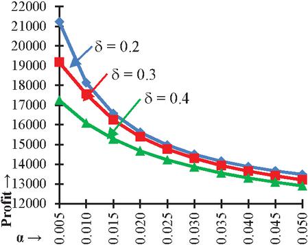
Figure 3

10 Conclusion

Table 1 and Figure 2 shows the behaviour of MTSF with respect to $\alpha$ for different values of $\delta$ i.e., 0.2, 0.3, and 0.4. From above table and graph, we observe that MTSF of the system model is decreasing with increasing $\alpha$. It is also clear that increment in $\delta$ decreases the MTSF. Initially, there is a significant decrease in MTSF and then it decreases at an approximate constant rate. Table 2 and Figure 3 reveals the behaviour of profit of the system model with respect to $\alpha$ for different values of $\delta$. The profit function also shows a significant decrease in profit and then it decreases gradually with increasing $\alpha$. We can conclude that MTSF and profit of the system model will be maximum for lower rate of change of weather conditions.

Further, MTSF and profit of the considered system model can be analysed with a different set of assumptions such as delay in the repair facility, replacement of the subsystem-A/subsystem-B, using fuzzy concept, etc.

References

Chachra, A., Kumar, A. and Ram, A., (2023): Intuitionistic fuzzy approach to reliability assessment of multi-state systems. Mathematics and Computers in Simulation, Vol. 212(C), 489–503.

Ghosh, Jyotishree, Pawar, D. and Malik, S.C. (2023): Performance analysis of a non-identical units system with inspection and operational priority. International Journal of Agricultural and Statistical Sciences, Vol. 19(Supplement 1), pp. 1169–1177.

Goel, L.R., Kumar, A. and Rastogi, A.K. (1985): Stochastic behaviour of man-machine systems operating under different weather conditions. Microelectronics Reliability, Vol. 25(1), pp. 87–91.

Goel, L.R., Sharma, G.C. and Gupta, P. (1986): Reliability analysis of a system with preventive maintenance, inspection and two types of repairs. Microelectronics Reliability, Vol. 26(3), pp. 429–433.

Gupta, R., Ramkishan and Goel, R. (1997): Analysis of a system having super-priority, priority and ordinary units with arbitrary distributions. Microelectronics Reliability, Vol. 37(5), pp. 851–856.

Kumar, A., Pawar, D. and Malik, S.C. (2019): Profit analysis of a warm standby non-identical unit system with single server performing in normal/abnormal environment. Life Cycle Reliability and Safety Engineering, Vol. 8(3), pp. 219–226.

Kumar, Lalit, Pawar, D. and Kumar, Kailash (2022): Cost-effectiveness analysis of a complex system with diverse repair policies under normal weather conditions. European Chemical Bulletin, Vol. 11(10), pp. 702–710.

Malik, S.C., Kadyan, M.S. and Grewal, A.S. (2004): Stochastic analysis of non-identical units reliability model with priority and different modes of failure. Journal of Decision and Mathematical Sciences, Vol. 9(1–3), pp. 59–82.

Malik, S.C., Raj, M., Thakur, R. (2023): Weighted correlation coefficient measure for intuitionistic fuzzy set based on cosine entropy measure. Springer, Vol. 15, pp. 3449–3461.

Murari, K. and Goyal, V. (1983): Reliability of a system with two types of repair facility. Microelectronics Reliability, Vol. 23(6), pp. 1015–1025.

Pawar, D., Malik, S.C. and Bahl, S. (2010A): Steady state analysis of an operating system with repair at different levels of damages subject to inspection and weather conditions. International Journal of Agricultural and Statistical Sciences, Vol. 6(1), pp. 225–234.

Pawar, D., Malik, S.C. and Kumar, Jitender (2010B): Analysis of a system working under different weather conditions with on-line repair and random appearance of the server at partial failure stage. International Journal of Statistics and Systems, Vol. 5(4), pp. 485–496.

Pawar, D., Malik, S.C. and Reetu (2013): Weathering server system operations. Indian Journal of Science and Technology, Vol. 6(10), pp. 5325–5330.

Ram, M., Negi, G., Goyal, N., Kumar, A., (2022): Analysis of a Stochastic Model with Rework system. Journal of Reliability and Statistical Studies, 15(2), 553–582.

Rander, M.C., Kumar, Ashok and Tuteja, R.K. (1992): A two-unit cold standby system with major and minor failures and preparation time in the case of major failure. Microelectronics Reliability, Vol. 32(9), pp. 1199–1204.

Rathee, Reetu, Pawar, D. and Malik, S.C. (2018): Reliability modeling and analysis of a parallel unit system with priority to repair over replacement subject to maximum operation and repair times. International Journal of Trend in Scientific Research and Development, Vol. 2(5), pp. 350–358.

Sehgal, Archana (2000): Study of some reliability models with partial failure, accidents and various types of repair. PhD Thesis, Department of Statistics, M.D. University, Rohtak, India.

Siwach, B.S., Singh, R.P., and Taneja, G. (2001): Reliability and profit evaluation of a two-unit cold standby system with instructions and accidents. Pure and Applied Mathematika Sciences, Vol. 53(1–2), pp. 23–31.

Taneja, G. and Naveen, V. (2003): Comparative study of two reliability models with patience time and chances of non-availability of an expert repairman. Pure and Applied Mathematika Sciences, Vol. 52(1–2), pp. 23–35.

Tuteja, R.K. and Taneja, Gulshan (1991): Cost-benefit analysis of a two-server, two-unit, warm standby system with different types of failure. Microelectronics Reliability, Vol. 32(10), pp. 1353–1359.

Biographies

Lalit Kumar received his bachelor’s degree in Statistics from University of Delhi in 2009, M.Sc. degree in Statistics from CCS University in 2012, and now he is pursuing his Doctor of Philosophy degree in Statistics from Amity University Uttar Pradesh, Noida. He is currently working as an Assistant Professor at the Department of Statistics, Ramjas College, University of Delhi. His research areas include reliability modeling and analysis.

D. Pawar received the bachelor’s degree in Statistics from M.D. University in 1998, M.Sc. degree in mathematical Statistics from M.D. University in 2000, M. Phil. degree in Statistics from M.D. University in 2002, and Ph.D. degree in Statistics from M.D. University in 2010. He is currently working as a Professor at the Department of Statistics, Amity Institute of Applied Sciences, Amity University Uttar Pradesh, Noida. His research areas include reliability modeling and analysis, and optimizations techniques. He has been serving as a reviewer for many highly reputed journals.

Kailash Kumar received his bachelor’s degree in Statistics from CCS University in 2002, M.Sc. degree in Statistics from CCS University in 2004, M.Phil. degree in Statistics from CCS University in 2005, and the Doctor of Philosophy degree in Statistics from CCS University in 2008. He is currently working as an Associate Professor at the Department of Statistics, Lady Shri Ram College for Women, University of Delhi. His research areas include reliability theory, and applied Statistics. He has been serving as a reviewer for many highly reputed journals.

Journal of Reliability and Statistical Studies, Vol. 17, Issue 2 (2024), 333–350.
doi: 10.13052/jrss0974-8024.1724
© 2024 River Publishers

Abstract

1 Introduction

2 Notations

3 Transition Probabilities and Mean Sojourn Times

3.1 Mean Sojourn Time $({\mathit{\psi }}_{\mathbf{i}})$ in State ${\mathbf{S}}_{\mathbf{i}}$ are

4 Reliability of the System and MTSF

5 Steady-State Availability

6 Busy Period Analysis

7 Cost-Benefit Analysis

8 Particular Case

9 Discussion

10 Conclusion

References

Biographies