A New Exponential Gompertz Distribution: Theory and Applications

Ibtesam Ali Alsaggaf

King Abdulaziz University, Department of Statistics, Faculty of Science, Jeddah, Saudi Arabia
E-mail: ialsaggaf@kau.edu.sa
https://orcid.org/0009-0004-6356-7095

Received 04 September 2024; Accepted 17 October 2024

Abstract

With the rise of numerous phenomena that require interpretation and investigation, developing novel distributions has become an important need. This research introduced a new probability distribution called New Exponential Gompertz distribution based on the new exponential-X family to enhance flexibility and improve performance. The most significant benefit of this novel distribution is that its hazard function could be increasing, decreasing and bathtub which reflects the flexibility of the distribution to fit various applications. Furthermore, its density can adopt a variety of symmetric and asymmetric possible shapes. Some of the theoretical characteristics such as quantile, order statistic and moment are provided. The parameter estimates are derived using five different estimation methods including maximum likelihood, ordinary least square, weighted least square, Cramér-von mises and maximum product of spacing methods. Simulation studies are conducted to assess the effectiveness of the five estimation methods. The maximum likelihood estimate shows the most reliable estimate for estimating parameters since it provides the smallest mean square error While the maximum product of spacing method is less efficient. The performance of the proposed distribution is assessed through real-world applications in medical, engineering and physics with competitive distributions. The results indicate that the new distribution efficiently represents various types of data compared to other distributions.

Keywords: Gompertz distribution, NEX family, Rényi entropy, maximum likelihood estimation, Ordinary least square method, weighted least square method, Cramér-von mises method, maximum product of spacing method, simulation.

1 Introduction

The Gompertz distribution is a probability distribution employed in survival analysis to model the distribution of lifetimes. It is a classical distribution that represents survival function based on fatality laws. This distribution is critical for predicting many phenomena related to life. It is essential for estimating death rates for humans and fitting financial data. The Gompertz distribution was proposed by [12]. It has been applied for growth models as well as for predicting tumor growth.

The cumulative function (CDF) of Gompertz is

$$F(x)=1-e^{-\frac{\lambda }{\beta }\left(e^{\beta x}-1\right)},x>0;\lambda ,\beta >0.$$

(1)

and its probability density function (PDF) is

$$f(x)=\lambda e^{\beta x}{e}^{-\frac{\lambda }{\beta }\left(e^{\beta x}-1\right)}$$

(2)

Although this distribution was good at representing several phenomena in some fields, its ability to represent many real phenomena is still limited because it tends to exhibit an exponentially rising failure rate over lifetime data. These limitations appear in most classical distributions such as exponential and Weibull distributions due to their limited hazard function shapes, which makes them unsuitable for certain applications. Over the years, several improvements and generalizations have been proposed to make the Gompertz distribution more flexible and useful in a variety of applications. [10] introduced the generalized Gompertz distribution with three parameters using the exponentiated method. Following that, [9] expanded [10] model by adding two more shape parameters to the model using the exponentiated generalized technique proposed by [8]. Aside from developing the Gompertz distribution, [2] provided Gompertz generalized family based on the $T-X$ transformation technique defined by [4]. The Gompertz Normal, Gompertz Beta, Gompertz Gamma, Gompertz Log-Logistic, Gompertz Exponentiated Weibul and Gompertz Lomax [23] all are developed distributions derived from [2].

[1] combined the Exponentiated method in [10] with Gompertz exponential derived from [2] to propose another generalized Gompertz distribution. This model gives more flexibility in modeling survival data. Another generation of Gumprtz is the Kumaraswamy-G generalized Gompertz distribution which was proposed by [11]. [24] provided the three parameters Gamma–Gompertz model which was derived by the gamma-X family. In 2024, [6] combined the odd Weibull family with the inverse Gompertz distribution to introduce a new family that merges the features of both distributions. At same year, [15] employed $T-X$ transformation to introduce a new model called the generalized Gompertz-G family. The primary objective of these efforts is to optimize the Gompertz distribution fitting in a way that it can seamlessly handle diverse real-world data across various domains. These generalizations were applied to a variety of data in engineering, medicine, physics, and other fields and various phenomena.

In a new attempt to improve Gompertz’s efficiency, this research aims to utilize an alternative method for generalizing distributions. In this study, a new generalization for the Gompertz distribution is developed by employing the new lifetime exponential-X family (NEX) proposed by [14]. This family is distinguished by its provision of a diverse array of hazard function forms.

The NEX family’s CDF and PDF are provided by:

$$G(x)=1-[1-F(x)]e^{-\theta F(x)},x>0;\theta ,>0.$$	(3)
$$g(x)=f(x)\left[\frac{1+\theta \left[1-F(x)\right]}{e^{\theta F(x)}}\right]$$	(4)

By integrating the attributes of this family with those of the Gumpertz distribution to represent reliability data, we can create a new distribution that encompasses all of these features. The aim of this article is to introduce a novel extension of the Gompertz distribution, known as the New Exponential Gompertz distribution (NEG), based on the NEX distribution family. The NEG distribution has several benefits:

• The NEG distribution expands on the Gompertz distribution by adding new parameters, which enhances its flexibility and allows for a more precise representation of different tail shapes.

• It increases the adaptability of density and hazard rate functions, enabling precise modeling of diverse real-world scenarios.

• It offers greater flexibility than the Gompertz distribution, resulting in a superior fit compared to other distributions.

• The CDF, hazard rate functions, moments, and entropy of the NEG distribution are all provided in closed form, making it a valuable tool for analyzing both complete and censored data.

• The hazard rate function for the NEG distribution exhibits a wide range of forms, including symmetrical and asymmetrical shapes in its density function. This flexibility enables NEG to effectively represent and analyze a diverse array of data from fields such as engineering, medicine, physics, and reliability.

This article is classified as follows: Section 2 describes the NEG using graphical representations. Section 2.1 gives useful expantion for the NEG’s CDF and PDF. Section 3 derived statistical properties for NEG. In section 4, five estimation methods are applied to estimate the NEG parameters: maximum likelihood (ML), ordinary least squares (O.LS), weighted least squares (W.LS), Cramér-von Mises (CRM) and maximum product of spacing (MPS). Section 5 presents assessing the performance of the estimation methods using Monte Carlo simulation technique. Section 6 analyzes various datasets of cancer patient data to evaluate the modeling effectiveness of the EFG distribution and compare it performance against competitive distributions. Section 7 concludes with some final remarks.

2 The New Exponential Gompertz Distribution (NEG)

The NEG’s CDF and PDF are founded by replacing the $G(x)$ and $g(x)$ in (3) and (4) by (1) and (2) as follows:

$$F(x)=1-\left[e^{-\frac{\lambda }{\beta }\left(e^{\beta x}-1\right)}\right]\left[e^{-\theta \left(1-e^{-\frac{\lambda }{\beta }\left(e^{\beta x}-1\right)}\right)}\right],$$	(5)
$$f(x)=\lambda e^{\beta x}{e}^{-\frac{\lambda }{\beta }\left(e^{\beta x}-1\right)}\left[\frac{1+\theta \left[e^{-\frac{\lambda }{\beta }\left(e^{\beta x}-1\right)}\right]}{e^{\theta \left[1-e^{-\frac{\lambda }{\beta }\left(e^{\beta x}-1\right)}\right]}}\right],$$	(6)

where $\lambda ,\beta ,\theta ,>0$, $x\ge 0$.

The Survival, $S(x)$ of NEG is expressed as

$$S(x)=\left[e^{-\frac{\lambda }{\beta }\left(e^{\beta x}-1\right)}\right]\left[e^{-\theta \left(1-e^{-\frac{\lambda }{\beta }\left(e^{\beta x}-1\right)}\right)}\right],$$

(7)

and its hazard rate functions, $hrf(x)$, is written as

$$hrf(x)=\lambda e^{\beta x}\left[1+\theta e^{-\frac{\lambda }{\beta }\left(e^{\beta x}-1\right)}\right].$$

(8)

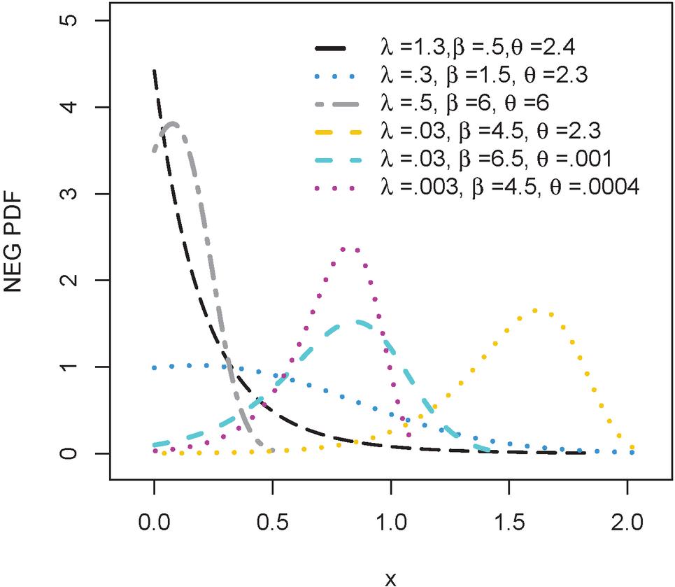
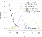
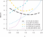
Figure 1 The density plots of NEG($\lambda$, $\beta$, $\theta$).

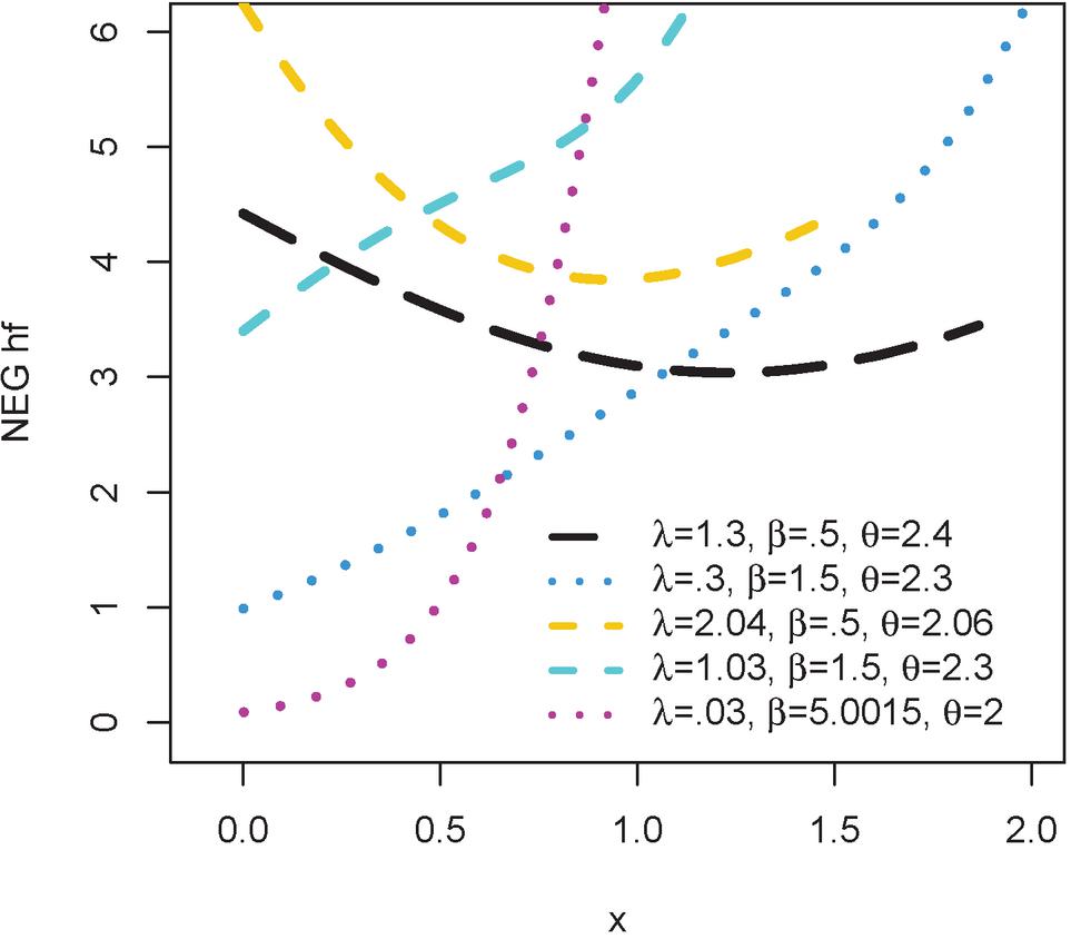
Figures 1 and 2 display several types of curves for NEG’s density and hrf at different combinations of the parameter values. Figure 1 shows the distinct shapes of the density distribution of NEG, as it oscillates from skewed to the right to skewed to the left. It also takes the J-shaped, in addition to the symmetrical shape.

Regarding the hazard rate function of NEG, Figure 2 shows that the hazard function has a wide range of shapes, including increasing, decreasing, J-shaped, and inverse J-shaped. This indicates the high flexibility of the distribution, which indicates the possibility of its compatibility with many phenomena.

A special sub-model of NEG is Gompertz distribution (2) when $\theta =0$.

Figure 2 The hazard plots for NEG ($\lambda$, $\beta$, $\theta$).

2.1 Additional Expression for the NEG’s CDF and PDF

Expansion for the NEG’s CDF and PDF given in Equations (5) and (6), respectively, are delivered in this subsection.

Using exponential expansion, see [22]:

$$e^{-z}=\sum _{k=0}^{\mathrm{\infty }}\frac{{(-1)}^k{(z)}^k}{k!},$$

(9)

The NEG’s PDF might then be written as

$F(x)$

$={\displaystyle \sum _{k_1=0}^{\mathrm{\infty }}}{\displaystyle \frac{{(-1)}^{k_1}}{k_1!}}{\theta }^{k_1}{e}^{-\frac{\lambda }{\beta }\left(e^{\beta x}-1\right)}{\left[1-e^{-\frac{\lambda }{\beta }\left(e^{\beta x}-1\right)}\right]}^{k_1}$

Further, applying the binomial series (10) for $m>0$ and $|r|<1$

$${(1-r)}^n=\sum _{m=0}^{\mathrm{\infty }}{(-1)}^m\left(\genfrac{}{}{0pt}{}{n}{m}\right)r^m$$

(10)

Thus, the NEG’s CDF can be reduced to

$F(x)$

$=1-{\eta }_1{\left[1-e^{-\frac{\lambda }{\beta }\left(e^{\beta x}-1\right)}\right]}^{k_1+m_1},$

(11)

where

${\eta }_1={\displaystyle \sum _{k_1=0}^{\mathrm{\infty }}}{\displaystyle \sum _{m_1=0}^1}{\displaystyle \frac{{(-1)}^{k_1+m_1}}{k_1!}}\left({\displaystyle \genfrac{}{}{0pt}{}{1}{m_1}}\right){\theta }^{k_1}$

(12)

To find the expansion for the NEG’S PDF, the series in Equations (9), (10) and (13) are employed.

$${(1+u)}^l=\sum _{i=0}^{\mathrm{\infty }}\left(\genfrac{}{}{0pt}{}{l}{i}\right)u^i.$$

(13)

Therefore, the NEG’s PDF can be reduced to

$f(x)$

$={\eta }_2{e}^{\beta (1+k_3)x},$

(14)

where

${\eta }_2={\displaystyle \sum _{i_1=0}^1}{\displaystyle \sum _{k_2=0}^{\mathrm{\infty }}}{\displaystyle \sum _{m_2=0}^j}{\displaystyle \sum _{k_3=0}^{\mathrm{\infty }}}{\displaystyle \frac{{(-1)}^{m_2+k_3}}{k_2!k_3!}}\left({\displaystyle \genfrac{}{}{0pt}{}{1}{i_1}}\right)\left({\displaystyle \genfrac{}{}{0pt}{}{n}{k_2}}\right)\left({\displaystyle \frac{{\lambda }^{k_3+1}}{{\beta }^{k_3}}}\right)$

${(m_2+i_1+1)}^{k_3}{\theta }^{(i_1+k_2)}{e}^{\frac{\lambda }{\beta }(m_2+i_1+1)}$

(15)

3 Statistical Properties of the NEG

Some fundamental properties of NEG such as quantile, moment, order statistic and more are driven in this section.

3.1 Quantile Function and Quartiles

The quantile function $(x_p)$ of the NEG might be written as

$$x_p=\frac{ln}{\beta }\left[1-\frac{\beta }{\lambda }ln\left(\frac{W(\theta e^{\theta }(1-p)}{\theta }\right)\right],0<p<1.$$

(16)

where W[·] is the Lambert function.

The median of the NEG distribution can be obtained as

$$x_{0.50}=\frac{ln}{\beta }\left[1-\frac{\beta }{\lambda }ln\left(\frac{W(\theta e^{\theta }(0.5)}{\theta }\right)\right]$$

Hence, the ${25}^{th}$ percentile and the ${75}^{th}$ percentile of the NEG distribution are given as

$x_{0.25}$	$={\displaystyle \frac{ln}{\beta }}\left[1-{\displaystyle \frac{\beta }{\lambda }}ln\left({\displaystyle \frac{W(\theta e^{\theta }(0.75)}{\theta }}\right)\right],$
$x_{0.75}$	$={\displaystyle \frac{ln}{\beta }}\left[1-{\displaystyle \frac{\beta }{\lambda }}ln\left({\displaystyle \frac{W(\theta e^{\theta }(0.25)}{\theta }}\right)\right].$

3.2 Shape Indices

The shape of the NEG can be measures by Galton’s skewness and Moors’ kurtosis [20] which are obtained by applying (16) and respectively given as follows:

$$\mathit{Skewness}=\frac{q_{0.75}-2q_{0.5}+q_{0.25}}{q_{0.75}-q_{0.25}},$$

(17)

and

$$\mathit{Kurtosis}=\frac{q_{0.875}-q_{0.625}+q_{0.375}-q_{0.125}}{q_{0.75}-q_{0.25}}.$$

(18)

Table 1 Mean, median, quartiles, skewness and kurtosis of the NEG for various values of $\lambda$, $\beta$ and $\theta$.

$\lambda$	$\beta$	$\theta$	$Q_1$	$Q_2$	Mean	$Q_3$	Skewness	Kurtosis
1.3	0.5	2.4	0.066	0.159	0.239	0.327	2.44	11.55
0.002	0.05	0.4	37.876	53.678	52.123	66.853	-0.24	2.577
3	2.2	1.6	0.037	0.087	0.125	0.168	1.773	6.641
9	10	3	0.009	0.02	0.027	0.036	1.907	8.149
0.03	2.7	7	0.556	0.84	0.822	1.091	-0.11	2.359
0.05	0.008	0.04	5.263	12.129	16.365	23.118	1.489	5.707
0.003	3.5	2.6	1.321	1.571	1.529	1.793	-0.584	3.444
0.33	0.005	0.004	0.876	1.991	2.907	3.951	1.932	7.791
0.55	0.89	0.27	0.35	0.719	0.824	1.201	0.721	2.909
1.5	3.2	4.5	0.034	0.077	0.107	0.153	1.598	6.368

For details see [3].

Table 1 shows some values of the mean, median ($Q_2$), first quartile ($Q_1$), third quartile ($Q_3$), skewness, and kurtosis for the NEG, for some different values the parameters $\lambda$, $\beta$ and $theta$. The table reveals a wide range of values represented by the distribution, with the mean and quartiles spanning from values below one to significantly larger values. Additionally, the measures of skewness indicate that the distribution can exhibit different degrees of skewness, ranging from right-skewed to left-skewed. The kurtosis values also indicate varying levels of tail width. Specifically, when the lambda parameter is less than 0.01, the distribution tends to be skewed to the left.

3.3 Moments

If $X$ follows the NEG ($\lambda$, $\beta$, $\theta$), then the $r^{th}$ moment of $X$ is written as

$$E\left(x^r\right)={\int }_0^{\mathrm{\infty }}{x}^{r}f(x)\mathit{d}x={\eta }_2{\int }_0^{\mathrm{\infty }}{x}^r{e}^{\beta (1+k_3)x}\mathit{d}x,$$

(19)

where ${\eta }_2$ is given by (2.1). Using Laplace transformation, $L_t\left[f(t)\right](s)={\int }_0^{\mathrm{\infty }}f(t)e^{-st}\mathit{d}t$ where $f(t)$ is defined for $t\ge 0$ [17], with taking $f(t)=t^r$ then $L_t\left[f(t)\right](s)=\frac{r!}{s^{r+1}}$, where $s=-\beta (1+k_3)$. Therefore,

$$E(x^r)={\eta }_{2}r!{\left(\frac{-1}{\beta (1+k_3)}\right)}^{r+1}$$

Thus, the $r^{th}$ moment is expressed as

$${\mu }_r=E\left(x^r\right)={\eta }_2{\left(\frac{-1}{\beta (1+k_3)}\right)}^{r+1}\mathrm{\Gamma }(r+1),r\ge 0$$

(20)

Then, the NEG’s mean is written as

$$\mu =E\left(x\right)={\eta }_2{\left(\frac{1}{\beta (1+k_3)}\right)}^2$$

(21)

The NEG’s variance is determined by

${\sigma }^2=$

$E(x^2)-{\mu }^2=2{\eta }_2{\left({\displaystyle \frac{-1}{\beta (1+k_3)}}\right)}^3-{\mu }^2,$

where ${\eta }_2$ is given by (2.1).

3.4 Moment Generating Function

If $X$ follows the NEG ($\lambda$, $\beta$, $\theta$), then the NEG’s moment generating function (MGF) is written as

$$M_x(t)=E(e^{tx})={\int }_0^{\mathrm{\infty }}{e}^{tx}f(x)\mathit{d}x={\eta }_2{\int }_0^{\mathrm{\infty }}{e}^{tx}{e}^{\beta (1+k_3)x}\mathit{d}x,$$

(22)

Using Laplace transformation, with taking $f(t)=1$ then $L_t\left[f(t)\right](s)=\frac{1}{s}$, where $s=-(t+\beta (1+k_3))$, then MGF will be given as

$$M_x(t)=E(e^{tx})={\eta }_2\left(\frac{-1}{t+\beta (1+k_3)}\right),$$

(23)

where ${\eta }_2$ is given by (2.1).

3.5 Characteristic Function

The characteristic function of NEG is simply constructed as:

${\varphi }_x\left(t\right)=$

$E(e^{itx})={\eta }_2\left({\displaystyle \frac{-1}{it+\beta (1+k_3)}}\right),$

(24)

where ${\eta }_2$ is given by (2.1).

3.6 Mean Residual Life and Mean Waiting Time

If $X\sim NEG(\lambda ,\beta ,\theta )$ with $S(t)$ provided in (7), then the mean residual life, $\mu (t)$, is expressed as

$$\mu (t)=\frac{1}{S(t)}\left(E(t)-{\int }_0^{t}xf(x)\mathit{d}x\right)-t.$$

(25)

If the incomplete moment, $I_{inc}={\int }_0^{t}xf(x)\mathit{d}x$, then

$$I_{inc}={\int }_0^t{\eta }_{2}x{e}^{\beta (1+k_3)x}\mathit{d}x.$$

Setting $y=\beta (1+m)x$, then simplifying will be obtained,

$$I_{inc}=\left(\frac{{\eta }_2}{{\beta }^2{(1+k_3)}^2}\right){\int }_0^{t\beta (1+k_3)}y{e}^y\mathit{d}y,$$

Using integration by part by taking $u=y$ and $dv=e^{y}dy$, the incomplete moment will be obtained as

$$I_{inc}=\left(\frac{{\eta }_2}{{\beta }^2{(1+k_3)}^2}\right)\left[\beta t(1+k_3)e^{\beta t(1+k_3)}-e^{\beta t(1+k_3)}+1\right],$$

(26)

Substituting (21), and (26) in (25), $\mu (t)$ might be rewritten as

$\mu (t)$

$={\displaystyle \frac{1}{S(t)}}{\displaystyle \frac{{\eta }_2}{{\beta }^2{(1+k_3)}^2}}\left[e^{\beta t(1+k_3)}-\beta t(1+k_3)e^{\beta t(1+k_3)}\right]-t,$

(27)

In a similar manner, the mean waiting time, $\overline{\mu }(t)$, might be defined as

$$\overline{\mu }(t)=t-\frac{1}{F(t)}{\int }_0^{t}xf(x)\mathit{d}x,$$

(28)

where $F(t)$ is provided in (11). Then, $\overline{\mu }(t)$ of the NEG can be found by substituting (11) and (26) in (28) as follows

$\overline{\mu }(t)$

$=t-{\displaystyle \frac{{\eta }_2}{{\beta }^2{(1+k_3)}^2}}\left[{\displaystyle \frac{\beta t(1+k_3)e^{\beta t(1+k_3)}-e^{\beta t(1+k_3)}+1}{1-{\eta }_1{\left[1-e^{-\frac{\lambda }{\beta }\left(e^{\beta x}-1\right)}\right]}^{k_1+m_1}}}\right]$

3.7 Rényi entropy

$R{E}_X(\zeta )$ is the Rényi entropy function which given as

$$R{E}_X(\zeta )=\frac{1}{1-\zeta }\log \left({\int }_0^{\mathrm{\infty }}f{(x)}^{\zeta }\mathit{d}x\right);\zeta >0,\zeta \ne 1.$$

Then, applying the NEG’s PDF in (6)

$f{(x)}^{\zeta }={\lambda }^{\zeta }{e}^{\zeta \beta x}{e}^{-\frac{\zeta \lambda }{\beta }\left(e^{\beta x}-1\right)}{\left[1+\theta \left(e^{-\frac{\lambda }{\beta }\left(e^{\beta x}-1\right)}\right)\right]}^{\zeta }\left[e^{-\zeta \theta \left(1-e^{-\frac{\lambda }{\beta }\left(e^{\beta x}-1\right)}\right)}\right].$

Applying the same approach in Subsection 2.1 and using (9), (13) and (10), then

$f{(x)}^{\zeta }={\eta }_2^{*}{e}^{(\zeta +k_5)\beta x},$

where

${\eta }_2^{*}={\displaystyle \sum _{i_2=0}^{\zeta }}{\displaystyle \sum _{k_4=0}^{\mathrm{\infty }}}{\displaystyle \sum _{m_3=0}^j}{\displaystyle \sum _{k_5=0}^{\mathrm{\infty }}}{\displaystyle \frac{{(-1)}^{j+k_5+m_3}}{j!k_5!}}\left({\displaystyle \genfrac{}{}{0pt}{}{\zeta }{i_2}}\right)\left({\displaystyle \genfrac{}{}{0pt}{}{j}{m_3}}\right)\left({\displaystyle \frac{{\lambda }^{\zeta +k_5}}{{\beta }^{k_5}}}\right)$

${(\zeta +m_3+i_2)}^{k_5}{\theta }^{(i_2+k_4)}{e}^{\frac{\zeta \lambda }{\beta }}.$

Using Laplace transformation, since $f(t)=1$ then $L_t[f(t)](s)=\frac{1}{s}$, where $s=-(\zeta +k_5)\beta$, then the Rényi entropy of the NEG, is then will be reduced to

$R{E}_x(\zeta )$

$={\displaystyle \frac{1}{1-\zeta }}\log \left[{\displaystyle \frac{-{\eta }_2^{*}}{(\zeta +k_5)\beta }}\right].$

3.8 Order Statistics

The density function, $f_{j:n}(x)$, of the $j^{th}$ order statistics is given as

$$f_{j:n}(x)=\frac{1}{B(j,n-j+1)}f(x){\left[F(x)\right]}^{j-1}{\left[1-F(x)\right]}^{n-j}.$$

(29)

By employing the binomial series formula in (10) to (29), $f_{j:n}(x)$ can be expressed as

$$f_{j:n}(x)=\frac{1}{B(j,n-j+1)}\sum _{m_3=0}^{n-j}{(-1)}^{m_3}\left(\genfrac{}{}{0pt}{}{n-j}{m_3}\right)f(x){\left[F(x)\right]}^{m_3+j-1}.$$

(30)

By substituting the CDF (11) and PDF of NEG (14) into (30), the PDF of $X_{j:n}$ is

$f_{j:n}(x)={\displaystyle \frac{\left[{\eta }_2{e}^{\beta (1+k_3)x}\right]}{B(j,n-j+1)}}{\displaystyle \sum _{m_3=0}^{n-j}}{(-1)}^{m_3}\left({\displaystyle \genfrac{}{}{0pt}{}{n-j}{m_3}}\right)$
${\left[1-{\eta }_1{\left[1-e^{-\frac{\lambda }{\beta }(e^{\beta x}-1)}\right]}^{k_1+m_1}\right]}^{m_3+j-1}$	(31)

where ${\eta }_1$ and ${\eta }_2$ are given by (12) and (2.1), respectively.

4 Estimation Methods

4.1 Maximum Likelihood Estimation (ML)

Assume $x_1,\mathrm{\dots },x_n$ is a random sample from $NEG(\lambda ,\beta ,\theta )$ with size n. Therefore, the log-likelihood function, ($\mathrm{\ell }$), for $(\lambda ,\beta ,\theta )$, is written as

$\mathrm{\ell }(\lambda ,\beta ,\theta )$	$={\displaystyle \sum _{i=1}^n}\ln \left({\mathrm{e}}^{-\frac{\lambda }{\beta }\left({\mathrm{e}}^{\beta x}-1\right)}\theta +1\right)-\theta {\displaystyle \sum _{i=1}^n}\left(1-{\mathrm{e}}^{-\frac{\lambda }{\beta }\left({\mathrm{e}}^{\beta x}-1\right)}\right)$
	$\mathrm{\hspace{1em}}-{\displaystyle \sum _{i=1}^n}{\displaystyle \frac{\lambda }{\beta }}\left({\mathrm{e}}^{\beta x_i}-1\right)+\beta {\displaystyle \sum _{i=1}^n}{x}_i+n\ln \left(\lambda \right)$	(32)

The derivation for the Equation (4.1) in regard to $\lambda ,\beta$ and $\theta ,$ are written as follows:

${\displaystyle \frac{\partial \mathrm{\ell }}{\partial \lambda }}$	$=-{\displaystyle \frac{\theta }{\beta }}{\displaystyle \sum _{i=1}^n}\left[{\displaystyle \frac{\left({\mathrm{e}}^{\beta x_i}-1\right){\mathrm{e}}^{-\frac{\lambda }{\beta }\left({\mathrm{e}}^{\beta x_i}-1\right)}}{\theta {\mathrm{e}}^{-\frac{\lambda }{\beta }\left({\mathrm{e}}^{\beta x_i}-1\right)}+1}}\right]$
	$\mathrm{\hspace{1em}}-{\displaystyle \frac{\theta }{\beta }}{\displaystyle \sum _{i=1}^n}\left[\left({\mathrm{e}}^{\beta x_i}-1\right){\mathrm{e}}^{-\left({\mathrm{e}}^{\beta x_i}-1\right)\lambda }\right]+{\displaystyle \frac{n}{\lambda }}-{\displaystyle \frac{1}{\beta }}\cdot {\displaystyle \sum _{i=1}^n}({\mathrm{e}}^{\beta x_i}-1),$	(33)
${\displaystyle \frac{\partial \mathrm{\ell }}{\partial \beta }}$	$={\displaystyle \sum _{i=1}^n}\left[{\displaystyle \frac{\frac{\theta \lambda }{\beta }\left({\displaystyle \frac{\left({\mathrm{e}}^{x_i\beta }-1\right)}{\beta }}-x_i{\mathrm{e}}^{x_i\beta }\right){\mathrm{e}}^{-\frac{\lambda }{\beta }\left({\mathrm{e}}^{x_i\beta }-1\right)}}{\theta {\mathrm{e}}^{-\frac{\lambda }{\beta }\cdot \left({\mathrm{e}}^{x\beta }-1\right)}+1}}\right]$
	$\mathrm{\hspace{1em}}+{\displaystyle \frac{\theta \lambda }{\beta }}{\displaystyle \sum _{i=1}^n}\left[\left({\displaystyle \frac{\left({\mathrm{e}}^{x_i\beta }-1\right)}{\beta }}-x_i{\mathrm{e}}^{x_i\beta }\right){\mathrm{e}}^{-\frac{\lambda }{\beta }\left({\mathrm{e}}^{x_i\beta }-1\right)}\right]$
	$\mathrm{\hspace{1em}}-{\displaystyle \frac{\lambda }{\beta }}{\displaystyle \sum _{i=1}^n}(x_i{\mathrm{e}}^{x_i\beta })+{\displaystyle \frac{\lambda }{{\beta }^2}}{\displaystyle \sum _{i=1}^n}\left({\mathrm{e}}^{x_i\beta }-1\right)+{\displaystyle \sum _{i=1}^n}{x}_i,$	(34)
${\displaystyle \frac{\partial \mathrm{\ell }}{\partial \theta }}$	$={\displaystyle \sum _{i=1}^n}\left[{\displaystyle \frac{{\mathrm{e}}^{-\frac{\lambda }{\beta }\left({\mathrm{e}}^{\beta x_i}-1\right)}}{\theta {\mathrm{e}}^{-\frac{\lambda }{\beta }\left({\mathrm{e}}^{\beta x_i}-1\right)}+1}}\right]+{\displaystyle \sum _{i=1}^n}\left[{\mathrm{e}}^{-\frac{\lambda }{\beta }\left({\mathrm{e}}^{\beta x_i}-1\right)}\right]-n,$	(35)

Therefore, the estimate for each parameter can be derived by setting (33), (34) and (35) to zero and numerically solving by Newton–Raphson iteration method which is available in R program. Furthermore, the log-likelihood present in (4.1) can be alternatively optimized using a non-linear optimization tool.

4.2 Ordinary Least Square Method (O.LS)

O.LS method is proposed by [25], which is based on the difference between the empirical and theoretical cdf. Suppose a random sample from NEG distribution with size n and $X_{(1)},X_{(2)},\mathrm{\dots },X_{(n)}$ are its order statistics. The sum of squares for the difference between the empirical and theoretical cdf of NEG distribution is formulated in Equation (36).

$$O.LS(\mathrm{\Theta })=\sum _{k=1}^n{\left[F(x_{(k)})-\left(\frac{k}{n+1}\right)\right]}^2$$

(36)

where the $F(x_{(k)})$ is the cdf of NEG and $\left(\frac{k}{n+1}\right)$ is the empirical cdf and $i=1,2,\mathrm{\dots },n$.

The partial derivation from the Equation (36) in regard to $\mathrm{\Theta }=(\lambda ,\beta ,\theta )$ can be written as follows:

$$\frac{\partial O.LS(\mathrm{\Theta })}{\partial \lambda }=\sum _{k=1}^n\left[F(x_{(k)})-\left(\frac{k}{n+1}\right)\right]\frac{\partial F(x_{(k)};\mathrm{\Theta })}{\partial \lambda }$$	(37)
$$\frac{\partial O.LS(\mathrm{\Theta })}{\partial \beta }=\sum _{k=1}^n\left[F(x_{(k)})-\left(\frac{k}{n+1}\right)\right]\frac{\partial F(x_{(k)};\mathrm{\Theta })}{\partial \beta }$$	(38)
$$\frac{\partial O.LS(\mathrm{\Theta })}{\partial \theta }=\sum _{k=1}^n\left[F(x_{(k)})-\left(\frac{k}{n+1}\right)\right]\frac{\partial F(x_{(k)};\mathrm{\Theta })}{\partial \theta }$$	(39)

where the $\frac{\partial F(x_{(k)};\mathrm{\Theta })}{\partial \lambda }$, $\frac{\partial F(x_{(k)};\mathrm{\Theta })}{\partial \beta }$ and $\frac{\partial F(x_{(k)};\mathrm{\Theta })}{\partial \theta }$ are given as

${\displaystyle \frac{\partial F(x_{(k)};\mathrm{\Theta })}{\partial \lambda }}$	$=-\left(-{\displaystyle \frac{\left({\mathrm{e}}^{x\beta }-1\right)\theta {\mathrm{e}}^{-\frac{\left({\mathrm{e}}^{x\beta }-1\right)\lambda }{\beta }}}{\beta }}-{\displaystyle \frac{{\mathrm{e}}^{x\beta }-1}{\beta }}\right)$
	$\mathrm{\hspace{1em}\hspace{1em}}{\mathrm{e}}^{-\theta \left(1-{\mathrm{e}}^{-\frac{\left({\mathrm{e}}^{x\beta }-1\right)\lambda }{\beta }}\right)-\frac{\left({\mathrm{e}}^{x\beta }-1\right)\lambda }{\beta }}$	(40)
${\displaystyle \frac{\partial F(x_{(k)};\mathrm{\Theta })}{\partial \beta }}$	$=-(\theta ({\displaystyle \frac{\lambda \left({\mathrm{e}}^{x\beta }-1\right)}{{\beta }^2}}-{\displaystyle \frac{x\lambda {\mathrm{e}}^{x\beta }}{\beta }})$
	$\mathrm{\hspace{1em}\hspace{1em}}{\mathrm{e}}^{-\frac{\lambda \left({\mathrm{e}}^{x\beta }-1\right)}{\beta }}-{\displaystyle \frac{x\lambda {\mathrm{e}}^{x\beta }}{\beta }}+{\displaystyle \frac{\lambda \left({\mathrm{e}}^{x\beta }-1\right)}{{\beta }^2}})$
	$\mathrm{\hspace{1em}\hspace{1em}}{\mathrm{e}}^{-\theta \left(1-{\mathrm{e}}^{-\frac{\lambda \left({\mathrm{e}}^{x\beta }-1\right)}{\beta }}\right)-\frac{\lambda \left({\mathrm{e}}^{x\beta }-1\right)}{\beta }}$	(41)
${\displaystyle \frac{\partial F(x_{(k)};\mathrm{\Theta })}{\partial \theta }}$	$=-\left({\mathrm{e}}^{-\frac{\left({\mathrm{e}}^{x\beta }-1\right)\lambda }{\beta }}-1\right){\mathrm{e}}^{-\left(1-{\mathrm{e}}^{-\frac{\left({\mathrm{e}}^{x\beta }-1\right)\lambda }{\beta }}\right)\theta -\frac{\left({\mathrm{e}}^{x\beta }-1\right)\lambda }{\beta }}$	(42)

The O.LS estimates for the parameters $\mathrm{\Theta }$ can be obtained by minimizing the Equation (36) concerning the $\mathrm{\Theta }=(\lambda ,\gamma ,\theta ,\beta ,\alpha )$ or by solving the equations from (37) to (39) using numerical techniques available in statistical software.

4.3 Weighted Least Square Method (W.LS)

WLS method is similar to OLS method, which depends on the differences between the empirical and theoretical of the cdf, in addition to the variance of the order statistic as a wight [25]. Therefore, the WLS function for NEG is written as

$$W.LS(\mathrm{\Theta })=\sum _{k=1}^n{\omega }_k{\left[F(x_{(k)})-\left(\frac{k}{n+1}\right)\right]}^2$$

(43)

where ${\omega }_k=\frac{{(n+1)}^2(n+2)}{k(n+1-k)}$

The Equation (43) is derived for each parameter in NEG distribution and the derivation equations are given as follows.

$$\frac{\partial W.LS(\mathrm{\Theta })}{\partial \lambda }=\sum _{k=1}^n{\omega }_k\left[F(x_{(k)})-\left(\frac{k}{n+1}\right)\right]\frac{\partial F(x_{(k)};\mathrm{\Theta })}{\partial \lambda }$$	(44)
$$\frac{\partial W.LS(\mathrm{\Theta })}{\partial \beta }=\sum _{k=1}^n{\omega }_k\left[F(x_{(k)})-\left(\frac{k}{n+1}\right)\right]\frac{\partial F(x_{(k)};\mathrm{\Theta })}{\partial \beta }$$	(45)
$$\frac{\partial W.LS(\mathrm{\Theta })}{\partial \theta }=\sum _{k=1}^n{\omega }_k\left[F(x_{(k)})-\left(\frac{k}{n+1}\right)\right]\frac{\partial F(x_{(k)};\mathrm{\Theta })}{\partial \theta }$$	(46)

where the $\frac{\partial F(x_{(k)};\mathrm{\Theta })}{\partial \lambda }$, $\frac{\partial F(x_{(k)};\mathrm{\Theta })}{\partial \beta }$ and $\frac{\partial F(x_{(k)};\mathrm{\Theta })}{\partial \theta }$ are given by (4.2), (4.2) and (42).

The W.LS estimation is obtained by minimizing the Equation (43) or by solving the nonlinear equations from (44) to (46) using numerical iterative technique available in any statistical software.

4.4 Cramér-von Mises Method (CRM)

[19] introduced the CRM method for estimation parameters. The function of the CRM method for NEG distribution is presented in Equation (47).

$$CRM(\mathrm{\Theta })=\frac{1}{12n}+\sum _{k=1}^n{\left[F(x_{(k)})-\left(\frac{2k-1}{2n}\right)\right]}^2$$

(47)

The equations below show the partial derivatives of the parameters $\mathrm{\Theta }=(\lambda ,\beta ,\theta )$ from (47). The CRM estimates for NEG parameters are derived by solving the equations from (48) to (50) using numerical technique or by minimizing (47) using optimization technique available in R Package.

$$\frac{\partial CRM(\mathrm{\Theta })}{\partial \lambda }=\sum _{k=1}^n\left[F(x_{(k)})-\left(\frac{2k-1}{2n}\right)\right]\frac{\partial F(x_{(k)};\mathrm{\Theta })}{\partial \lambda }$$	(48)
$$\frac{\partial CRM(\mathrm{\Theta })}{\partial \beta }=\sum _{k=1}^n\left[F(x_{(k)})-\left(\frac{2k-1}{2n}\right)\right]\frac{\partial F(x_{(k)};\mathrm{\Theta })}{\partial \beta }$$	(49)
$$\frac{\partial CRM(\mathrm{\Theta })}{\partial \theta }=\sum _{k=1}^n\left[F(x_{(k)})-\left(\frac{2k-1}{2n}\right)\right]\frac{\partial F(x_{(k)};\mathrm{\Theta })}{\partial \theta }$$	(50)

where the $\frac{\partial F(x_{(k)};\mathrm{\Theta })}{\partial \lambda }$, $\frac{\partial F(x_{(k)};\mathrm{\Theta })}{\partial \beta }$ and $\frac{\partial F(x_{(k)};\mathrm{\Theta })}{\partial \theta }$ are given by (4.2), (4.2) and (42).

4.5 Maximum Product of Spacing Method (MPS)

[7] proposed MPS method in order to improve the performance of the ML estimator. Let a random sample from NEG distribution with size n and $x_{(1)},x_{(2)},\mathrm{\dots },x_{(n)}$ is the corresponding ordered sample. The idea of MPS method is to optimize the geometric mean of spacings, which refers to the variations between the cdf values of adjacent data points. The spacings between neighboring ordered values can be defined as $D_k(\mathrm{\Theta })=F(x_{(k)};\mathrm{\Theta })-F(x_{(k-1)};\mathrm{\Theta }),\mathrm{\Theta }=(\lambda ,\gamma ,\theta ,\beta ,\alpha ),k=1,\mathrm{\dots },n+1.$

Therefore, the MPS function for NEG is given as

$M(\mathrm{\Theta })$	$={\displaystyle \frac{1}{n+1}}{\displaystyle \sum _{k=1}^{n+1}}log{D}_k(\mathrm{\Theta })$
$M(\mathrm{\Theta })$	$={\displaystyle \frac{1}{n+1}}{\displaystyle \sum _{k=1}^{n+1}}log\left[F(x_{(k)})-F(x_{(k-1)})\right]$	(51)

The first partial derivative of (51) with respect to $\mathrm{\Theta }=(\lambda ,\beta ,\theta )$, are given as follows. The MPS estimates for NEG parameters are derived by solving the equations from (52) to (54) using numerical technique or via maximizing (51) using optimization technique available in R Package.

$$\frac{\partial M(\mathrm{\Theta })}{\partial \lambda }=\frac{1}{n+1}\sum _{k=1}^{n+1}\left[\frac{F_{\lambda }^{\prime }(x_{(k)})-F_{\lambda }^{\prime }(x_{(k-1)})}{F(x_{(k)})-F(x_{(k-1)})}\right]$$	(52)
$$\frac{\partial M(\mathrm{\Theta })}{\partial \beta }=\frac{1}{n+1}\sum _{k=1}^{n+1}\left[\frac{F_{\beta }^{\prime }(x_{(k)})-F_{\beta }^{\prime }(x_{(k-1)})}{F(x_{(k)})-F(x_{(k-1)})}\right]$$	(53)
$$\frac{\partial M(\mathrm{\Theta })}{\partial \theta }=\frac{1}{n+1}\sum _{k=1}^{n+1}\left[\frac{F_{\theta }^{\prime }(x_{(k)})-F_{\theta }^{\prime }(x_{(k-1)})}{F(x_{(k)})-F(x_{(k-1)})}\right]$$	(54)

where the $F_{\lambda }^{\prime }(.)$, $F_{\beta }^{\prime }(.)$ and $F_{\theta }^{\prime }(.)$ are given by (4.2), (4.2) and (42).

5 Simulation Study

Five techniques of estimation including ML, O.LS, W.LS, CRM and MPS are performed to calculate the estimation for the NEG parameters using Monte Carlo Simulation. Different sample sizes and three different sets of parameter values are applied.

The samples are drawn from the NEG distribution of size 15, 30, 50, 100 and 200 for the following three parameter sets:

• Set I: ($\lambda$= 1.3, $\beta$= 0.5, $\theta$= 2.4).

• Set II: ($\lambda$= 0.002, $\beta$= 0.05, $\theta$= 0.4).

• Set III: ($\lambda$= 3, $\beta$= 2.2, $\theta$= 1.6).

The sample of size n is generated N=1000 times. For each sample, the parameters estimates are calculated using the five estimation methods. Then, the average estimates, bias and the mean squared error (MSE) are calculated for each parameter.

Table 2 to 4 display the result of the simulation. The tables show ML, O.LS, W.LS, CRM and MPS estimate values for each parameter and corresponding bias and MSE. The results in the tables show that, as the sample size increases, the MSE generally decreases for all five methods, indicating improved accuracy with more data. Additionally, parameter estimates themselves tend to converge towards the true values. The performance of the methods O.LS, W.LS, CRM and MPS are similar in terms of the MSE values. However, the MPS is considered less efficient as it has large MSE values at some parameter estimation. Out of all the estimators, the ML estimator has the lowest MSE values. Consequence of this, ML is the most reliable choices for estimating NEG parameters.

Table 2 Parameter estimation, MSE and Bias from five different methods (Set I).

		Set I: ($\lambda$=1.3, $\beta$=0.5, $\theta$=2.4)
n	Par.	ML	O.LS	W.LS	CRM	PMS
15	$\widehat{\lambda }$	2.0315	2.0965	2.0287	1.9939	1.9659
	Bias	0.9380	1.3056	1.28572	1.2125	1.2459
	MSE	1.1828	1.7872	1.6709	1.7411	1.5485
	$\widehat{\beta }$	1.3751	0.3436	0.5011	1.4022	0.1726
	Bias	1.2476	2.0975	1.9022	2.3226	1.3904
	MSE	1.8491	2.9236	2.5878	3.5417	1.7854
	$\widehat{\theta }$	1.2539	2.7795	3.1570	2.5601	7.7718
	Bias	1.219	2.1898	2.5882	2.0646	7.4249
	MSE	1.3448	3.3806	4.4675	3.3194	17.3591
30	$\widehat{\lambda }$	1.9242	1.9454	1.8694	1.9698	1.7217
	Bias	0.7500	1.1428	1.1266	1.0991	1.1011
	MSE	0.9908	1.4746	1.4421	1.5316	1.3023
	$\widehat{\beta }$	0.9335	0.3171	0.4352	0.7756	0.0186
	Bias	0.7803	1.3455	1.1854	1.3583	0.9379
	MSE	1.1328	1.7181	1.5599	1.8139	1.1376
	$\widehat{\theta }$	1.4466	2.6318	2.9034	2.2815	8.0858
	Bias	1.0605	1.9492	2.1671	1.6949	7.3997
	MSE	1.2061	2.6649	3.1662	2.3049	15.5624
50	$\widehat{\lambda }$	1.8082	1.8812	1.7861	1.9048	1.6348
	Bias	0.6432	1.04919	1.0433	1.0238	1.0042
	MSE	0.8075	1.2911	1.2959	1.2896	1.1727
	$\widehat{\beta }$	0.7495	0.3324	0.3750	0.6132	0.0746
	Bias	0.5563	0.9945	0.8434	0.9970	0.7198
	MSE	0.7799	1.2617	1.09143	1.3045	0.8739
	$\widehat{\theta }$	1.6319	2.4849	2.8776	2.2484	6.6048
	Bias	0.9846	1.7485	2.0619	1.5776	5.7493
	MSE	1.1212	2.1691	2.7127	1.9714	12.0264
100	$\widehat{\lambda }$	1.7262	1.8554	1.7409	1.8517	1.5115
	Bias	0.5724	0.9762	0.9498	0.9502	0.8544
	MSE	0.7389	1.2304	1.1533	1.2174	1.0234
	$\widehat{\beta }$	0.6012	0.3280	0.3522	0.4700	0.1605
	Bias	0.3733	0.6932	0.5741	0.6822	0.5071
	MSE	0.4806	0.8657	0.7269	0.8684	0.6213
	$\widehat{\theta }$	1.8060	2.3345	2.6560	2.2417	5.0841
	Bias	0.8842	1.5409	1.7784	1.4465	3.9542
	MSE	1.0341	1.7584	2.0669	1.6683	8.1207
200	$\widehat{\lambda }$	1.4833	1.8526	1.7399	1.8444	1.4345
	Bias	0.3315	0.9244	0.9126	0.8983	0.7449
	MSE	0.4550	1.1442	1.1119	1.1219	0.9028
	$\widehat{\beta }$	0.5674	0.3237	0.3183	0.3989	0.2195
	Bias	0.2551	0.5019	0.3972	0.4914	0.3731
	MSE	0.3263	0.6166	0.4919	0.6083	0.4558
	$\widehat{\theta }$	2.1560	2.1987	2.5417	2.1440	4.0119
	Bias	0.6403	1.4297	1.6477	1.3605	2.6925
	MSE	0.7821	1.5585	1.8109	1.4949	4.8025

Table 3 Parameter estimation, MSE and Bias from five different methods (Set II)

		Set II: ($\lambda$=0.002, $\beta$=0.05, $\theta$=0.4)
n	Par.	ML	O.LS	W.LS	CRM	PMS
15	$\widehat{\lambda }$	0.0022	0.0032	0.0031	0.0026	0.0033
	Bias	0.0005	0.0022	0.0022	0.0018	0.0021
	MSE	0.0009	0.0029	0.0029	0.0025	0.0029
	$\widehat{\beta }$	0.0496	0.0459	0.0466	0.0527	0.0439
	Bias	0.0007	0.0139	0.0132	0.0142	0.0119
	MSE	0.0033	0.0177	0.0167	0.01913	0.0146
	$\widehat{\theta }$	0.4000	0.8008	0.8341	0.7595	0.7724
	Bias	$7.1\times {10}^{-6}$	0.9919	1.0302	0.9396	0.9411
	MSE	$2.9\times {10}^{-5}$	1.1804	1.2266	1.1158	1.1818
30	$\widehat{\lambda }$	0.0021	0.0029	0.0028	0.0025	0.0028
	Bias	0.0003	0.0018	0.0018	0.0016	0.0017
	MSE	0.0005	0.0024	0.0022	0.0019	0.0022
	$\widehat{\beta }$	0.04980	0.0468	0.0475	0.0502	0.0457
	Bias	0.0002	0.0103	0.0098	0.0101	0.0089
	MSE	0.0016	0.0128	0.0119	0.0128	0.0109
	$\widehat{\theta }$	0.4000	0.7592	0.8273	0.7509	0.9064
	Bias	$1.4\times {10}^{-6}$	0.9801	1.0462	0.9429	1.0548
	MSE	$9.8\times {10}^{-6}$	1.1479	1.2502	1.1083	1.3762
50	$\widehat{\lambda }$	0.0021	0.0027	2.1517	0.0026	0.0027
	Bias	0.0002	0.0016	0.6994	0.0015	0.0016
	MSE	0.0004	0.0020	1.1158	0.0019	0.0021
	$\widehat{\beta }$	0.0498	0.0476	0.3849	0.0489	0.0464
	Bias	0.0001	0.0082	0.1398	0.0083	0.0077
	MSE	0.0011	0.0099	0.1966	0.0103	0.0092
	$\widehat{\theta }$	0.4000	0.8056	1.3172	0.6798	0.9524
	Bias	$9.7\times {10}^{-7}$	1.0022	0.6025	0.8615	1.0896
	MSE	$9.5\times {10}^{-6}$	1.2436	0.8795	1.0358	1.5024
100	$\widehat{\lambda }$	0.0020	0.0026	0.0025	0.0025	0.0024
	Bias	0.0001	0.0015	0.0014	0.0014	0.0014
	MSE	0.0002	0.0018	0.0018	0.0017	0.0018
	$\widehat{\beta }$	0.0499	0.0476	0.0483	0.0487	0.0477
	Bias	0.0001	0.0069	0.0066	0.0067	0.0062
	MSE	0.0002	0.0083	0.0079	0.0081	0.0075
	$\widehat{\theta }$	0.3999	0.7149	0.7637	0.6930	1.0069
	Bias	$4.9\times {10}^{-7}$	0.8727	0.9011	0.8338	1.0845
	MSE	$2.2\times {10}^{-6}$	1.0413	1.1381	0.9928	1.5686
200	$\widehat{\lambda }$	0.0021	0.0026	0.0026	0.0025	0.0024
	Bias	$8.8\times {10}^{-5}$	0.0014	0.0013	0.0013	0.0013
	MSE	$1.4\times {10}^{-4}$	0.0016	0.0017	0.0016	0.0016
	$\widehat{\beta }$	0.0499	0.0476	0.0479	0.0481	0.0480
	Bias	$3.6\times {10}^{-5}$	0.0058	0.0057	0.0057	0.0051
	MSE	$2.6\times {10}^{-4}$	0.0069	0.0068	0.0068	0.0064
	$\widehat{\theta }$	0.3999	0.6235	0.6042	0.6210	0.9270
	Bias	$2.4\times {10}^{-7}$	0.7702	0.7480	0.7534	0.9689
	MSE	$1.2\times {10}^{-6}$	0.9273	0.9533	0.9147	1.5688

Table 4 Parameter estimation, MSE and Bias from five different methods.Set III

		Set III: ($\lambda$=3, $\beta$=2.2, $\theta$=1.6)
n	Par.	ML	O.LS	W.LS	CRM	PMS
15	$\widehat{\lambda }$	3.9322	4.3582	4.2387	4.1921	3.8708
	Bias	1.4051	2.5085	2.5473	2.4046	2.2388
	MSE	2.4254	3.5843	3.6015	3.5199	2.8925
	$\widehat{\beta }$	3.8863	1.6668	1.9058	3.6254	1.2220
	Bias	2.6651	4.0830	3.7259	4.3677	2.8072
	MSE	3.6928	5.5261	5.4303	6.3735	3.5693
	$\widehat{\theta }$	1.0210	2.0309	2.3391	2.0002	6.5198
	Bias	0.9275	1.7119	2.0173	1.7641	6.1664
	MSE	1.2258	2.9075	3.4730	3.3698	19.1609
30	$\widehat{\lambda }$	3.6988	3.9450	3.7604	3.8534	3.5659
	Bias	1.2542	2.1257	2.0994	2.0490	1.8882
	MSE	1.5303	2.7173	2.7858	2.6625	2.1896
	$\widehat{\beta }$	2.9954	1.5525	1.7536	2.5062	1.3431
	Bias	1.6886	2.6041	2.2638	2.6468	1.8356
	MSE	2.3045	3.3284	2.9826	3.5060	2.3013
	$\widehat{\theta }$	1.1767	1.9432	2.1947	1.8704	3.8317
	Bias	0.7988	1.4772	1.6692	1.4056	3.3037
	MSE	0.9342	1.8631	2.3645	1.9858	8.6487
50	$\widehat{\lambda }$	3.5703	3.8595	3.7238	3.8216	3.3875
	Bias	1.1732	1.9669	1.9595	1.8917	1.6775
	MSE	1.4371	2.2982	2.2877	2.2546	1.9340
	$\widehat{\beta }$	2.5994	1.6458	1.7512	2.1884	1.4693
	Bias	1.1939	1.9547	1.6447	1.9264	1.3618
	MSE	1.5871	2.4575	2.0605	2.4781	1.6699
	$\widehat{\theta }$	1.3045	1.7989	1.9632	1.7068	2.6875
	Bias	0.7949	1.3445	1.4894	1.2569	2.0296
	MSE	0.9902	1.5895	1.7479	1.5092	4.1732
100	$\widehat{\lambda }$	3.3079	3.8279	3.6028	3.8005	3.1955
	Bias	0.8619	1.8947	1.8400	1.8255	1.5130
	MSE	1.0235	2.1977	2.0587	2.0985	1.7332
	$\widehat{\beta }$	2.3920	1.6920	1.7822	1.9717	1.6057
	Bias	0.7654	1.4484	1.2057	1.4104	0.9854
	MSE	1.0026	1.7729	1.4632	1.7393	1.1895
	$\widehat{\theta }$	1.5261	1.7063	1.9394	1.6455	2.4444
	Bias	0.6711	1.2482	1.3998	1.1866	1.6472
	MSE	0.8241	1.3583	1.5782	1.3023	2.4673
200	$\widehat{\lambda }$	3.2362	3.7742	3.6352	3.7493	3.1166
	Bias	0.8826	1.8009	1.7777	1.7573	1.4572
	MSE	1.0504	2.0324	1.9913	1.9899	1.6681
	$\widehat{\beta }$	2.2067	1.7354	1.7847	1.8816	1.6800
	Bias	0.5499	1.0961	0.9211	1.0674	0.7436
	MSE	0.7088	1.3263	1.1181	1.3020	0.9055
	$\widehat{\theta }$	1.6225	1.6818	1.8469	1.6535	2.4265
	Bias	0.7027	1.1868	1.2991	1.1479	1.5679
	MSE	0.8863	1.2611	1.4379	1.2183	2.1053

6 Real-life Data Applications

Five real-world dataset from different disciplines in medicine, engineering, and physics are employed to illustrate the flexibility and efficiency of the NEG as a lifetime model. The first dataset comprised the survival times of 121 breast cancer patients who were treated at a major hospital between 1929 and 1938 [18]. The second dataset included 36 patients and recorded the periods of remission in months for individuals with bladder cancer [13]. This third dataset consisted of the lifetime (in years) of 40 blood cancer (leukemia) patients from one of the Ministry of Health hospitals in Saudi Arabia [5]. The fourth dataset was provided by [16]. The data involved 59 items which reflects the electrical relay failure time (in hours) for a test conductor. The fifth dataset describes the fracture toughness for different materials [21].

Table 5 The Performance of NEG for Dataset I (Breast cancer data).

Distributions	NEG	GG	EGoE	Gompertz	R	E
Estimates	$\widehat{\lambda }=$ 0.008	$\widehat{\lambda }=$ 0.029	$\widehat{\lambda }=$ 1.430	$\widehat{\lambda }=$ 0.016	$\widehat{\lambda }=$ 41.113	$\widehat{\lambda }=$ 0.515
	(0.004)	(0.009)	(0.401)	(.002)	(1.869)	(0.086)
	$\widehat{\beta }=$ 0.014	$\widehat{\beta }=$ 0.002	$\widehat{\beta }=$ 2.380	$\widehat{\beta }=$0.011
	(0.003)	(0.004)	(0.867)	(0.002)
	$\widehat{\theta }=$ 0.845	$\widehat{\theta }=$ 1.752	$\widehat{\theta }=$ 0.726
	(0.767)	(0.398)	(0.106)
			$\widehat{\gamma }=$ 0.006
			(0.001)
$-\mathrm{\ell }$	579.218	580.974	583.599	583.765	600.989	585.128
AIC	1164.44	1167.949	1175.197	1171.530	1203.98	1172.255
CAIC	1168.629	1172.142	1180.789	1174.325	1205.378	1173.653
BIC	1172.823	1176.336	1186.38	1177.121	1206.776	1175.051
W*	0.100	0.099	0.329	0.332	1.539	0.459
AD*	0.734	0.832	1.942	2.5082	11,381	2.693
KS	0.057	0.078	0.105	0.098	0.198	0.120
p-value	0.828	0.447	0.136	0.194	.0001	0.060

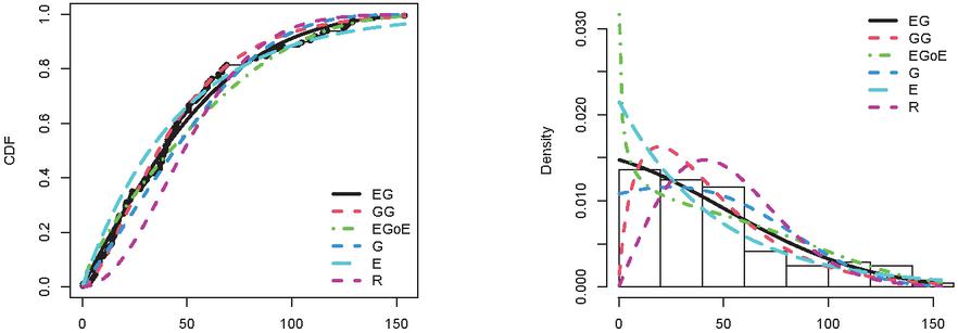
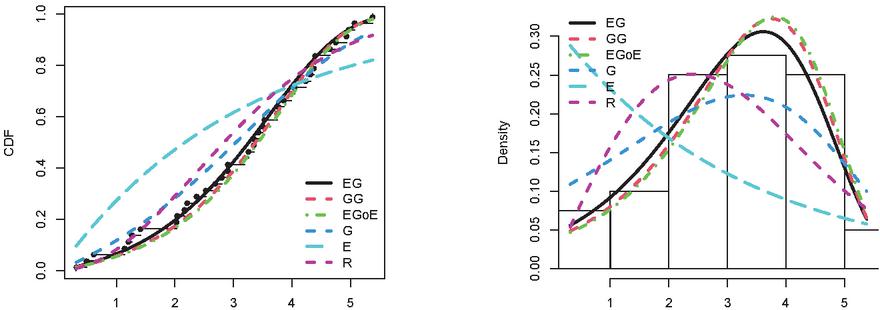
Figure 3 Empirical CDFs and PDFs for Dataset II (Breast cancer data).

The NEG model is compared with the exponential (E), Rayleigh (R), Gompertz (G), generalized Gompertz distribution (GG) [10], Exponentiated Gompertz Exponential (EGoG) [1].

The performance of the NEG is assessed using several goodness of fit indexes (GoF). The negative likelihood value ($-\mathrm{\ell }$), Akaike information criterion (AIC), corrected AIC (CAIC), Bayesian information criterion (BIC), Kramér-von Mises (W*) test statistic, Anderson-Darling (AD*) test statistic, Kolmogorov-Smirnov (KS) test statistic and associated p-value are employed in order to compare the proposed test with the competitive models. A model is considered to be the best in representing data when the values associated with these statistics are less than those of competing models.

Table 6 The Performance of NEG for Dataset II (Bladder cancer data).

Distributions	NEG	GG	EGoE	Gompertz	R	E
Estimates	$\widehat{\lambda }=$ 0.015	$\widehat{\lambda }=$ 0.779	$\widehat{\lambda }=$ 5.891	$\widehat{\lambda }=$ 2.369	$\widehat{\lambda }=$ 1.536	$\widehat{\lambda }=$ 0.515
	(0.014)	(0.619)	(2.145)	(0.164)	(0.128)	(0.086)
	$\widehat{\beta }=$ 1.051	$\widehat{\beta }=$ 0.108	$\widehat{\beta }=$ 12.172	$\widehat{\beta }=$0.004
	(0.217)	(0.394)	(12.995)	(0.002)
	$\widehat{\theta }=$ 6.161	$\widehat{\theta }=$ 2.445	$\widehat{\theta }=$ 1.425
	(6.569)	(1.390)	(0.742)
			$\widehat{\gamma }=$ 0.049
			(0.004)
$-\mathrm{\ell }$	47.522	53.619	48.645	66.089	51.399	59.857
AIC	101.044	113.238	105.291	136.179	104.797	121.714
CAIC	103.419	115.614	108.458	137.762	105.589	122.505
BIC	105.79	117.989	111.625	139.346	106.381	123.297
W*	0.084	0.299	0.159	1.089	0.172	0.656
AD*	0.547	1.662	0.886	11.758	1.121	3.408
KS	0.102	0.213	0.153	0.333	0.162	0.230
p-value	0.845	0.212	0.366	0.001	0.301	0.044

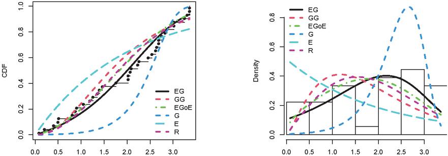
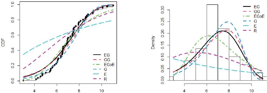
Figure 4 Empirical CDFs and PDFs for Dataset II (Bladder cancer data).

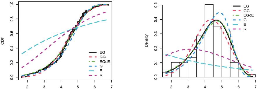
The Tables from 5 to 9 report the MLEs and the standard error corresponding with the GoF measurements of NEG and competitive distributions. The tables show that, the performance of the classical distributions fluctuated depending on the type of data. The exponential, Rayleigh, Gompertz distributions did not fit all the data, as they showed a significant p-value $<$ 0.05. As for modern distributions, such as GG and EGoG, the p-value $>$ 0.05, which means that these distributions are able to represent the data. Although these models fit the five datasets (p-value$\mathrm{>}$0.05), the NEG has the highest p-value among all the fitted models. Moreover, the Tables demonstrate that the NEG achieved the minimum values for all GoF indices. This indicates that the NEG distribution suits all five datasets better than the other competitive distributions.

The estimated PDF and CDF of NEG and the other models are presented in Figures from 3 to 7. The histogram represents the empirical density for the data and the dot black line represents the empirical CDF for the data. The Figures demonstrate that NEG closely aligns with the actual distribution of the datasets under examination. Therefore, when contrasted with alternative distributions, the NEG model emerges as the most suitable choice for the analyzed data.

Table 7 The Performance of NEG for Dataset III (Blood cancer data).

Distributions	NEG	GG	EGoE	gompertz	R	E
Estimates	$\widehat{\lambda }=$ 0.039	$\widehat{\lambda }=$ 0.033	$\widehat{\lambda }=$ 0.062	$\widehat{\lambda }=$ 0.503	$\widehat{\lambda }=$ 2.415	$\widehat{\lambda }=$ 0.318
	(0.075)	(0.031)	(0.044)	(0.113)	(0.191)	(0.050)
	$\widehat{\beta }=$ 0.812	$\widehat{\beta }=$ 0.859	$\widehat{\beta }=$ 1.821	$\widehat{\beta }=$0.096
	(0.367)	(0.223)	(0.710)	(0.031)
	$\widehat{\theta }=$ 0.123	$\widehat{\theta }=$ 0.965	$\widehat{\theta }=$ 0.949
	(1.594)	(0.366)	(0.299)
			$\widehat{\gamma }=$ 0.482
			(0.140)
$-\mathrm{\ell }$	65.778	65.810	65.881	68.281	70.806	85.778
AIC	137.556	137.620	139.762	140.563	143.612	173.556
CAIC	140.089	140.154	143.139	142.252	144.456	174,401
BIC	142.623	142.687	146.517	143.940	145.301	175.245
W*	0.027	0.034	0.047	0.118	0.250	1.084
AD*	0.211	0.282	0.358	0.719	1.297	5.479
KS	0.066	0.079	0.083	0.112	0.158	0.300
p-value	0.995	0.944	0.994	0.701	0.277	0.001

Figure 5 Empirical CDFs and PDFs for Dataset III (Blood cancer data).

Table 8 The pERFORMANCE of NEG for Dataset IV (electrical relay failure time).

(in hours) for a test conductor.

Distributions	NEG	GG	EGoE	Gompertz	R	E
Estimates	$\widehat{\lambda }=$ 0.003	$\widehat{\lambda }=$ 0.004	$\widehat{\lambda }=$ 0.019	$\widehat{\lambda }=$ 0.674	$\widehat{\lambda }=$ 5.064	$\widehat{\lambda }=$ 0.143
	(0.001)	(0.002)	(0.018)	(0.034)	(0.329)	(0.019)
	$\widehat{\beta }=$ 0.636	$\widehat{\beta }=$ 0.615	$\widehat{\beta }=$ 0.001	$\widehat{\beta }=$ 0.003
	(0.038)	(0.049)	(0.003)	(0.001)
	$\widehat{\theta }=$ 1.015	$\widehat{\theta }=$ 0.890	$\widehat{\theta }=$ 15.847
	(0.615)	(0.165)	(5.936)
			$\widehat{\gamma }=$ 21.560
			(12.855)
$-\mathrm{\ell }$	115.614	117.938	117.006	118.151	137.412	173.641
AIC	237.228	241.877	242.013	240.303	276.825	349.281
CAIC	240.345	244.993	246.168	242.380	277.864	350.319
BIC	243.461	248.109	250.323	244.458	278.902	351.359
W*	0.165	0.235	0.264	0.332	1.708	3.431
AD*	1.107	1.461	1.672	1.714	1.708	3.431
KS	0.108	0.130	0.114	0.162	0.313	0.430
p-value	0.465	0.248	0.399	0.080	$1.2\times {10}^{-05}$	$1.9\times {10}^{-10}$

Figure 6 Empirical CDFs and PDFs for Dataset IV (Electrical failure time).

Table 9 The Performance of NEG for the Dataset V (Fracture toughness).

Distribution	NEG	GG	EGoE	Gompertz	R	E
Estimates	$\widehat{\lambda }=$ 0.002	$\widehat{\lambda }=$ 0.151	$\widehat{\lambda }=$ 0.011	$\widehat{\lambda }=$ 1.213	$\widehat{\lambda }=$ 3.141	$\widehat{\lambda }=$ 0.231
	(0.0003)	(.096)	(0.005)	(0.040)	(0.144)	(0.021)
	$\widehat{\beta }=$ 1.192	$\widehat{\beta }=$ 0.451	$\widehat{\beta }=$ 0.960	$\widehat{\beta }=$ 0.003
	(0.044)	(0.135)	(0.356)	(0.001)
	$\widehat{\theta }=$ 0.843	$\widehat{\theta }=$ 5.030	$\widehat{\theta }=$ 1.157
	(0.416)	(2.649)	(0.215)
			$\widehat{\gamma }=$ 1.008
			(0.336)
$-\mathrm{\ell }$	170.142	170.294	170.719	173.534	221.035	293.275
AIC	346.283	346.588	349.437	351.068	444.069	588.551
CAIC	350.452	350.757	354.996	353.847	445.459	589.941
BIC	354.621	354.926	360.554	356.626	446.848	591.330
W*	0.089	0.103	0.113	0.246	3.421	6.716
AD*	0.547	0.818	0.690	1.305	17.274	32.261
KS	0.065	0.076	0.068	0.105	0.299	0.396
p-value	0.701	0.501	0.632	0.143	$1.2\times {10}^{-9}$	$1.1\times {10}^{-16}$

Figure 7 Empirical CDFs and PDFs for Dataset V (Fracture toughness).

7 Conclusions

In this paper, the NEG model is generated from Gompertz distribution based on NEX family. This distribution is designed to give greater adaptability and fit data from real life. The NEG’s density and hazard functions of NEG possess appealing shapes that can be used to fit various data patterns. Number of mathematical properties of the NEG model are described in detail including exact formulations for the density, moments, quantile order statistics and Rényi entropy. The ML, O.LS, W.LS, CRM and PMS estimations of the parameters are derived as well as assessed via simulation studies. ML is the most reliable estimate for estimating NEG parameters since it provides the smallest MSE compared to other estimates. The O.LS, W.LS, CRM, and MPS estimates exhibit similar performance regarding MSE values. While, MPS is considered as less efficient due to its higher MSE values in certain parameter estimations. Five different applications in medical, engineering and physics are used to assess the proposed model. The foremost eminent perspective is that NEG is a more suitable model than several competing models since it provides the smallest value for several GoF criteria. This illustrates that NEG exceeds all other competitor models in regard to execution and flexibility when conducted on different datasets. Based to these results, the NEG model could be useful for modeling other types of data in various area.

In future work, we plan to extend the application of the NEG model to additional domains and data types to further assess its versatility and robustness. This will include exploring its performance in other fields beyond medical, engineering, and physics, such as finance and social sciences, to evaluate its adaptability to diverse datasets. We will also investigate the potential of integrating the NEG model with other advanced estimation techniques, including Bayesian approaches, to improve parameter estimation and model fitting. Additionally, we aim to develop methods for handling complex censoring mechanisms and assess the model’s performance with various types of lifetime data. Enhancing the model’s computational efficiency and conducting real-world case studies will also be a focus, with the goal of refining the model’s applicability and providing more comprehensive insights into its practical utility across different applications.

Appendix

# ############################################

#PDF

dEG= func t i on ( x , a , b , t h )

{d=exp (−( a / b ) * ( exp ( b*x ) −1) )

f f =a *exp ( b*x ) *d* ( ( 1 + ( t h *d ) ) / exp ( t h *(1−d ) ) )

r e turn ( f f )

}

# ############################################

#CDF

pEG= func t i on ( q , a , b , t h )

{

x=q

d=exp (−( a / b ) * ( exp ( b*x ) −1) )

316 Ibtesam Ali Alsaggaf

F=1−(d*exp(−t h *(1−d ) ) )

r e turn ( F )

}

# ############################################

# q u a n t i l e NEG

qEG= func t i on ( n , a , b , t h )

{

u= runi f ( n , 0 , 1 )

z= t h *exp ( t h ) *(1−u )

d= l o g ( lambertWp ( z ) / t h )

F= l o g (1 −( ( b / a ) *d ) ) / b

r e turn ( F )

}

# ############################################

# L i k l i h o o d

l h = func t i on ( par , x ){

a=par [ 1 ] ; b=par [ 2 ] ; t h =par [ 3 ]

L=sum( l o g (dEG( x , a , b , t h ) ) )

r e turn (−L)}

# ############################################

## S imu l a t i o n

n =15; #n =(3 0 ,5 0 ,10 0 ,2 0 0 )

NS=1000

o p t t h =c ( )

o p t a=c ( )

o p t b=c ( )

s t a r t =c ( a , b , t h )

# ############################################

sample=qEG( n* 1000 , a=a , b=b , t h = t h )

x= matrix ( sample , nrow = NS, ncol =n )

f o r ( i i n 1 :NS) # i =1

{

o p t = optim ( par = s t a r t , fn = lh , x = x [ i , ] ) ;

o p t a [ i ]= o p t $par [ 1 ]

o p t b [ i ]= o p t $par [ 2 ]

o p t t h [ i ]= o p t $par [ 3 ]

New Exponential Gompertz Distribution 317

}

# ############################################

MLH a . h = mean ( o p t a )

MLH b . h = mean ( o p t b )

MLH t h . h = mean ( o p t t h )

MLH.EG. h=c (MLH a . h ,MLH b . h ,MLH t h . h )

#### #### ####

Bi a s a . h = mean ( abs ( o p t a − a ) )

Bi a s b . h = mean ( abs ( o p t b − b ) )

Bi a s t h . h = mean ( abs ( o p t t h − t h ) )

Bi a s .EG. h=c ( Bi a s a . h , Bi a s b . h , Bi a s t h . h )

#### #### ####

MSE a . h = sqr t (mean ( ( o p t a − a ) ˆ 2 ) )

MSE b . h = sqr t (mean ( ( o p t b − b ) ˆ 2 ) )

MSE t h . h = sqr t (mean ( ( o p t t h − t h ) ˆ 2 ) )

MSE.EG. h=c (MSE a . h ,MSE b . h ,MSE t h . h )

# ############################################

}

References

[1] A. Ademola, J. Adeyeye, M. Khaleel, and A. Olubisi. Exponentiated gompertz exponential (egoe) distribution: Derivation, properties and applications. Istatistik Journal of the Turkish Statistical Association, 13(1):12–28, 2021.

[2] M. Alizadeh, G. M. Cordeiro, L. G. B. Pinho, and I. Ghosh. The gompertz-g family of distributions. Journal of statistical theory and practice, 11:179–207, 2017.

[3] A. Alzaatreh, C. Lee, and F. Famoye. A new method for generating families of continuous distributions. Metron, 71(1):63–79, 2013.

[4] A. Alzaatreh, C. Lee, and F. Famoye. A new method for generating families of continuous distributions. Metron, 71(1):63–79, 2013.

[5] M. Atallah, M. Mahmoud, and B. Al-Zahrani. A new test for exponentiality versus nbumgf life distributions based on laplace transform. Quality and Reliability Engineering International, 30(8):1353–1359, 2014.

[6] L. A. Baharith. New generalized weibull inverse gompertz distribution: Properties and applications. Symmetry, 16(2):197, 2024. 318

[7] R. Cheng and N. Amin. Maximum product-of-spacings estimation with applications to the lognormal distribution. Math report, 791, 1979.

[8] G. M. Cordeiro, E. M. Ortega, and D. C. da Cunha. The exponentiated generalized class of distributions. Journal of Data Science, 11(1):1–27, 2013.

[9] T. A. De Andrade, S. Chakraborty, L. Handique, and F. Gomes-Silva. The exponentiated generalized extended gompertz distribution. Journal of Data Science, 17(2):299–330, 2019.

[10] A. El-Gohary, A. Alshamrani, and A. N. Al-Otaibi. The generalized gompertz distribution. Applied mathematical modelling, 37(1-2):13–24, 2013.

[11] Z. K. Ezmareh and G. Yari. Kumaraswamy-g generalized gompertz distribution with application to lifetime data. International Journal of Industrial Engineering, 33(4):1–22, 2022.

[12] B. Gompertz. Xxiv. on the nature of the function expressive of the law of human mortality, and on a new mode of determining the value of life contingencies. in a letter to francis baily, esq. frs &c. Philosophical transactions of the Royal Society of London, (115):513–583, 1825.

[13] R. Hibatullah, Y. Widyaningsih, and S. Abdullah. Marshall-olkin extended power lindley distribution with application. J. Ris. and Ap. Mat, 2(2):84–92, 2018.

[14] X. Huo, S. K. Khosa, Z. Ahmad, Z. Almaspoor, M. Ilyas, and M. Aamir. A new lifetime exponential-x family of distributions with applications to reliability data. Mathematical Problems in Engineering, 2020:1–16, 2020.

[15] J. Y. Kajuru, H. D. Garba, A. M. Suleiman, and A. F. Ibrahim. The generalized gompertz-g family of distributions: Statistical properties and applications. UMYU Scientifica, 3(1):120–128, Mar. 2024.

[16] A. A. Khalaf et al. [0, 1] truncated exponentiated exponential gompertz distribution: Properties and applications. In AIP Conference Proceedings, volume 2394. AIP Publishing, 2022.

[17] G. A. Korn and T. M. Korn. Mathematical handbook for scientists and engineers: definitions, theorems, and formulas for reference and review. Courier Corporation, 2000.

[18] E. T. Lee and J. Wang. Statistical methods for survival data analysis, volume 476. John Wiley & Sons, 2003.

[19] P. Macdonald. Estimation procedure for mixture distributions. Journal of the royal society series B- statistical methodology, 33(2):326–+, 1971.

[20] J. Moors. A quantile alternative for kurtosis. Journal of the Royal Statistical Society: Series D (The Statistician), 37(1):25–32, 1988.

[21] S. Nadarajah and S. Kotz. On the alternative to the weibull function. Engineering fracture mechanics, 74(3):451–456, 2007.

[22] M. Nassar, A. Alzaatreh, M. Mead, and O. Abo-Kasem. Alpha power weibull distribution: Properties and applications. Communications in Statistics-Theory and Methods, 46(20):10236–10252, 2017.

[23] P. E. Oguntunde, M. A. Khaleel, M. T. Ahmed, A. O. Adejumo, O. A. Odetunmibi, et al. A new generalization of the lomax distribution with increasing, decreasing, and constant failure rate. Modelling and Simulation in Engineering, 2017, 2017.

[24] M. Shama, S. Dey, E. Altun, and A. Z. Afify. The gamma–gompertz distribution: Theory and applications. Mathematics and Computers in Simulation, 193:689–712, 2022.

[25] J. J. Swain, S. Venkatraman, and J. R. Wilson. Least-squares estimation of distribution functions in johnson’s translation system. Journal of Statistical Computation and Simulation, 29(4):271–297, 1988.

Biography

Ibtesam Ali Alsaggaf received his B.Sc. and M.Sc. degrees from the Statistics department at King Abdulaziz University and Ph.D. degrees from the School of Mathematics at Universiti Sains Malaysia, Penang, in 2013. She is currently an assistant professor at the Statistics Department at King Abdulaziz University. She has published articles in International journals. Her fields of interest are Distribution theory and modeling.

Journal of Reliability and Statistical Studies, Vol. 17, Issue 2 (2024), 289–320.
doi: 10.13052/jrss0974-8024.1722
© 2024 River Publishers