Length Biased Weighted Ishita Distribution and Its Applications on Real Life Data Sets

Narinder Pushkarna and Mustafa^*

Department of Statistics, Ramjas College, University of Delhi–110007, India
E-mail: narinderpushkarna@ramjas.du.ac.in; mustafa@stats.du.ac.in
*Corresponding Author

Received 22 August 2024; Accepted 08 April 2025

Abstract

In this paper, we introduce a new extension within the realm of statistical distributions, presenting the “length-biased Ishita distribution.” This distribution stands out as part of the esteemed category of weighted distributions, particularly the length-biased variation. Through meticulous analysis, we explore the mathematical and statistical properties of this novel distribution and reveal its distinct characteristics. Using the robust methodology of maximum likelihood estimation, we accurately estimate the model parameters, enhancing our understanding of its behavior. To demonstrate the practical utility and advantages of the length-biased Ishita distribution, we apply it to a real-world temporal dataset. This empirical analysis highlights its superior performance and adaptability, offering valuable insights into its potential applications across various domains.

Keywords: Ishita distribution, length-biased distribution, new weighted length-biasedIshita distribution, parameter estimation.

Abbreviations

LBIs	Length Biased Ishita
LBWIs	Length Biased Weighted Ishita
LBT	Length Biased Tornumonkpe
PDF	Probability Density Function
CDF	Cumulative Density Function
MGF	Moment Generating Function
CF	Characteristic Function
DS 1	Data Set 1
DS 2	Data Set 2
DS 3	Data Set 3

1 Introduction

Weighted distributions stand as a potent remedy to tackle biases within unevenly sampled data, offering a holistic framework to model and depict statistical information. This notion, initially conceived by Fisher [1], explores the impact of finding methods on observed distributions. Subsequently, Rao [2] refined and unified this theory, particularly addressing scenarios where standard distributions struggle in noting the observations with balanced probabilities. Weighted distributions guide us in selecting the most suitable models for real-world data, especially when it’s unclear how the data was collected. By assigning more importance to certain observations based on specific factors, they help ensure our analysis reflects reality more accurately. A well-known type of weighted distribution is the length-biased distribution, where the weight is determined simply by the length of the items being studied.

The inventive work of Cox [3] and Zelen [4] introduced the concept of length-biased sampling, which has since found widespread application across diverse biomedical domains. From family history analysis to clinical trials, reliability theory to population studies, the utility of length-biased distributions is evident. Several published studies have explored length-biased distributions, including the works of Rather and Subramanian [5, 6, 8], Rather and Ozel [7], and Rather et al. [9]. In 2017, the Lindley distribution was extended by Shankar [10], which brought the Ishita distribution into existence for modeling lifetime data in biomedical science and engineering. Further advancements and applications of this distribution can be found in the works of Shukla et al. [11], Hassan et al. [12]. Ahmed et al. [13] introduced a length-biased weighted Lomax distribution (LBWLD) with maximum likelihood estimation for parameter estimation. Saghir et al. [14] proposed a Maxwell length-biased distribution, detailing its statistical properties and estimation methods. Ganaie et al. [15] developed the LBWNQLD, estimating parameters via maximum likelihood and demonstrating its application with real data. Dey et al. [16] analyzed the weighted inverted Weibull distribution, comparing parameter estimation methods. Mansoor et al. [17] presented the Lindley negative-binomial distribution, covering parameter estimation and real data applications. Ali et al. [18] compared Bayesian and frequentist methods for the Poisson Nadarajah-Haghighi (PNH) distribution. Chaito et al. [19] introduced the LBWR distribution, showing its superiority in hydrological datasets. Ogunde [20] presented the half-logistic Generalized Rayleigh distribution for lifetime data. Chesneau [21] proposed a modified weighted exponential distribution, outperforming existing models in real data applications. Hashempour [22] introduced the weighted Half-Logistic (WHL) distribution, demonstrating its better fit through simulations. Roshni [23] characterized the Generalized Area-Biased Power Ishita Distribution (GAPID), while Ferreira [24] discussed the exponentiated power Ishita distribution and its regression model with real data.

This paper aims to develop a new length-biased weighted distribution, which is the length-biased weighted Ishita (LBWIs) distribution, a new model designed to be highly flexible and applicable to a variety of real-world scenarios. What makes the LBWIs distribution particularly appealing is its ability to handle a wide range of data patterns. This versatility makes it especially useful for complex datasets commonly found in fields like survival analysis, reliability modeling, and hydrology, where length-biased sampling is often encountered.

The rest of this paper is organized as follows: In Sections 2 & 3, the proposed distribution is introduced. In Section 4, reliability measures, mathematical & statistical properties are derived. Parameter estimation is obtained in Section 5, along with the estimations of the information criteria. In Section 6, the proposed distribution is applied to three real-life datasets, and the reliability was evaluated for the proposed distribution and compared with other distributions. Conclusions and discussions are presented in Section 7.

2 Length Biased Distribution

If X is a non-negative random variable with the probability density function (PDF) $f (x)$ , then the corresponding weighted distribution $f_{w} (x)$ is given by;

f_{w} (x) = \frac{w (x) f (x)}{E {w (x)}}

(1)

Where $W (x)$ is a non-negative weighted function and $E {w (X)} < \infty$ , (cf. Fisher [1]).

Patil and Ord [25] presented a size-biased distribution that is a special case of the weighted distribution. The weighted function of a size-biased distribution is $W (X) = X^{c}$ , where $c = 1$ named length biased distributions is.

f_{LBIs} (x) = \frac{x f (x)}{E {X}}

(2)

Many length-biased distributions have been proposed in the literature. For example, Das and Roy [26, 27] studied the length-biased weighted generalized Rayleigh distribution and the length-biased weighted Weibull distribution, respectively. Ratnaparkhi and Naik–Nimbalkar [28] used the length-biased lognormal distribution. Khadim and Hussein [29] introduced the length-biased weighted Exponential and Rayleigh distributions for industrial data.

3 The Length-Biased Weighted Ishita (LBWIs) Distribution

The probability density function (PDF) of Ishitadistribution {proposed by Shankar and Shukla [10]} is given by:

f (x) = \frac{θ^{3}}{(θ^{3} + 2)} (θ + x^{2}) \exp (- θ x), x > 0, θ > 0

(3)

And the cumulative distribution function (CDF) of Ishita distribution is given by:

F (x) = 1 - [1 + \frac{θ x (θ x + 2)}{(θ^{3} + 2)}] \exp (- θ x), x > 0, θ > 0

(4)

Utilising Equation (2), for f(x) defined in Equation (3) we defined the PDF of LBWIs distribution;

Definition 1. A random variable X is said to have the length-biased weighted Ishita (LBWIs) distribution, if the PDF of X is

f_{LBWIs} (x) = \frac{θ^{4}}{(θ^{3} + 6)} x (θ + x^{2}) \exp (- θ x), x > 0, θ > 0

(5)

One can observe that the proposed LBWIs distribution can be regarded as Mixture of $γ (2, θ)$ and $γ (4, θ)$ with factor $α = \frac{θ^{3}}{(θ^{3} + 6)}$ .

The corresponding cumulative distribution function (CDF) of X is obtained by

F_{LBWIs} (x) = 1 - {(θ^{4} x + θ^{3} x^{3} + 3 θ^{2} x^{2} + 6 θ x + θ^{3} + 6)} \frac{\exp (- θ x)}{(θ^{3} + 6)}

(6)

For $X > 0, θ > 0$

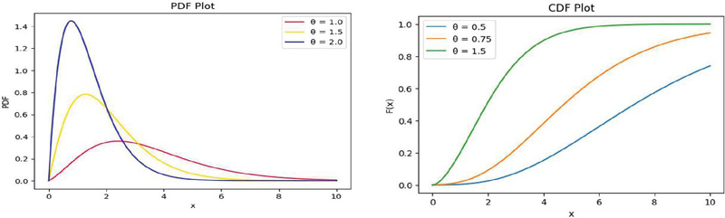
Figure 1 shows the PDF and CDF plots of the LBWIs distribution for different values of the parameter.

Figure 1 The probability density function (PDF) and cumulative distribution function (CDF) of the LBWIs distribution for different value of parameter $θ$ .

4 Reliability Measure and Mathematical Properties

In this section, we present the reliability measures, statistical and mathematical properties of the LBWIs distribution.

4.1 Reliability Measures

Here, the survival function, known as the reliability function; and the hazard function, known as the failure rate of the LBWIs distribution are presented. Since the reliability function can be obtained as

$R (x)$	$= 1 - F (x)$
$R_{LBWIs} (x)$	$= {(θ^{4} x + θ^{3} x^{3} + 3 θ^{2} x^{2} + 6 θ x + θ^{3} + 6)} \frac{\exp (- θ x)}{(θ^{3} + 6)}$	(7)

The hazard function is given by

$h (x)$	$= \frac{f (x)}{R (x)}$
$h_{LBWIs} (x)$	$= \frac{θ^{4} x}{{(θ^{4} x + θ^{3} x^{3} + 3 θ^{2} x^{2} + 6 θ x + θ^{3} + 6)}}$	(8)

To study the shape of hazard function; let $ζ (x) = - \frac{d}{d x} {\log f (x)}$ then

\frac{d}{d x} {ζ (x)} = \frac{1}{x} + \frac{2 x}{(θ + x^{2})} - θ > 0

(9)

The Reverse Hazard Function of LBWIs Distributions is given as

$h^{r} (x)$	$= \frac{f (x)}{F (x)}$
$h_{LBWIs}^{r} (x)$	$= \frac{θ^{4} x (θ + x^{2}) \exp (- θ x)}{\begin{matrix} [(θ^{3} + 6) - {(θ^{4} x + θ^{3} x^{3} + 3 θ^{2} x^{2} + 6 θ x + θ^{3} + 6)} \\ \exp (- θ x)] \end{matrix}}$	(10)

And the Mills Ratio of the LBWIs Distribution is given as

$h (x)$	$= \frac{\bar{F} (x)}{f (x)}$
$h_{MR, LBWIs} (x)$	$= \frac{{(θ^{4} x + θ^{3} x^{3} + 3 θ^{2} x^{2} + 6 θ x + θ^{3} + 6)}}{θ^{4} x}$	(11)

Figure 2 shows various Reliability, Hazard, Reverse Hazard and Mills Ratio plot of the LBWIs distribution with different parameter values.

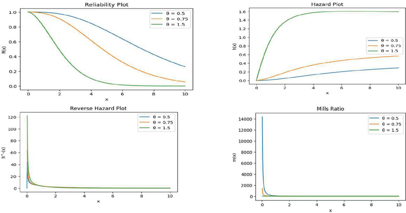
Figure 2 The reliability function (RF), hazard function (HF), reverse hazard function & Mills ratio of the LBWIs distribution for different value of parameter $θ$ .

4.2 Moment Generating Function (MGF), Characteristic Function (CF) and Cumulant Generating Function

In this subsection, we present the moment generating function, characteristic function and cumulant generating function which can be used for estimation of parameter of LBWIs distribution.

Let X is a LBWIs random variable with parameters ( $θ$ ). Then the moment generating function (MGF), characteristic function (CF) and cumulant generating function (CGF) of X $(X \neq 0)$ , is given in Equations (4.1) and (4.1) and Figure 3 show the plot of the Moment Generating Function (MGF), Characteristic Function (CF) and cumulant generating function (CGF).

$M_{X} (t)$	$= \frac{θ^{4} {θ {(θ - x)}^{2} + 6}}{(θ^{3} + 6) {(θ - x)}^{4}}$	(12)
$ψ_{X} (t)$	$= \frac{θ^{4} {θ {(θ - x i)}^{2} + 6}}{(θ^{3} + 6) {(θ - x i)}^{4}}$	(13)
$K_{X} (t)$	$= \ln [\frac{θ^{4} {θ {(θ - x)}^{2} + 6}}{(θ^{3} + 6) {(θ - x)}^{4}}]$	(14)

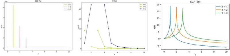
Figure 3 The MGF, CF, CGF of the LBWIs distribution for different value of parameter $θ$ .

4.3 Statistical Properties

In this subsection, we present the Mean, Harmonic Mean, Variance, Mean Deviation about Mean and Mean Deviation about Median.

Let X is a LBWIs random variable with parameters ( $θ$ ). Then the Mean ( $μ$ ), Harmonic Mean, Variance ( $σ^{2}$ ), Mean Deviation about Mean ${τ_{1} (x)}$ and Mean Deviation about Median ${τ_{2} (x)}$ is given as:

$E (X)$	$= μ = \frac{2 (θ^{3} + 12)}{θ (θ^{3} + 6)}$	(15)
$H . M (X)$	$= \frac{(θ^{3} + 6)}{θ (θ^{3} + 2)}$	(16)
$V (X)$	$= \frac{6 (θ^{3} + 20) (θ^{3} + 6) - 4 {(θ^{3} + 12)}^{2}}{θ^{2} {(θ^{3} + 6)}^{2}}$	(17)
$τ_{1} (X)$	$= \frac{2}{(θ^{3} + 6)} [\frac{2 (θ^{3} + 12)}{θ} F (μ)$
	$- {\begin{matrix} 24 + 2 θ^{2} - μ^{2} θ^{4} \exp (- θ μ) - 2 μ θ^{3} \exp (- θ μ) \\ - 2 θ^{2} \exp (- θ μ) - μ^{4} θ^{3} \exp (- θ μ) \\ - 4 μ^{3} θ^{2} \exp (- θ μ) - 12 μ^{2} θ \exp (- θ μ) \\ - 24 μ \exp (- θ μ) - \frac{24}{θ} \exp (- θ μ) \end{matrix}}]$	(18)
$τ_{2} (X)$	$= \frac{2}{(θ^{3} + 6)} [\frac{(θ^{3} + 12)}{θ}$
	$- {\begin{matrix} 24 + 2 θ^{2} - M^{2} θ^{4} \exp (- θ M) - 2 M θ^{3} \exp (- θ M) \\ - 2 θ^{2} \exp (- θ M) - M^{4} θ^{3} \exp (- θ M) \\ - 4 M^{3} θ^{2} \exp (- θ M) - 12 M^{2} θ \exp (- θ M) \\ - 24 M \exp (- θ M) - \frac{24}{θ} \exp (- θ M) \end{matrix}}]$	(19)

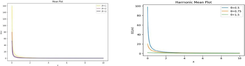
Figure 4

And the Figure 4 shows the Mean and Harmonic Mean plot for the different values of the parameter $θ$ .

4.4 Moments about Origin, Moments about Mean & Pearson’s $β$ and $γ$ Coefficients

The r $^{th}$ moment about the origin of the LBWIs distribution is written as

E (x^{r}) = [\frac{{θ^{3} Γ (r + 2) + Γ (r + 4)}}{θ^{r} (θ^{3} + 6)}]

(20)

Thus, the first four moments about the origin for X are

$E (X)$	$= μ_{1}^{'} = \frac{2 (θ^{3} + 12)}{θ (θ^{3} + 6)}$	(21)
$E (X^{2})$	$= μ_{2}^{'} = \frac{6 (θ^{3} + 20)}{θ^{2} (θ^{3} + 6)}$	(22)
$E (X^{3})$	$= μ_{3}^{'} = \frac{24 (θ^{3} + 30)}{θ^{3} (θ^{3} + 6)}$	(23)
$E (X^{4})$	$= μ_{4}^{'} = \frac{120 (θ^{3} + 42)}{θ^{4} (θ^{3} + 6)}$	(24)

The r $^{th}$ moment about the mean of X by using the relations between moments about mean in terms of moments about origin, we get the following moments about mean:

$μ_{1}$	$= 0$
$μ_{2}$	$= \frac{6 (θ^{3} + 20) (θ^{3} + 6) - 4 {(θ^{3} + 12)}^{2}}{θ^{2} {(θ^{3} + 6)}^{2}} = V (x)$	(25)
$μ_{3}$	$= \frac{\begin{matrix} 120 (θ^{3} + 42) {(θ^{3} + 6)}^{2} - 432 (θ^{3} + 30) (θ^{2} + 20) (θ^{3} + 6) \\ + 432 {(θ^{2} + 20)}^{3} \end{matrix}}{θ^{3} (θ^{3} + 6)}$	(26)
$μ_{4}$	$= \frac{\begin{matrix} 720 θ^{3} (θ^{3} + 56) {(θ^{3} + 6)}^{5} - 2880 θ^{2} (θ^{3} + 20) (θ^{3} + 42) {(θ^{3} + 6)}^{4} \\ + 5184 θ^{2} (θ^{3} + 30) {(θ^{3} + 20)}^{3} {(θ^{3} + 6)}^{3} - 3888 {(θ^{3} + 20)}^{4} \end{matrix}}{θ^{6} {(θ^{3} + 6)}^{6}}$	(27)

Karl Pearson’s coefffients based upon the first four moments about mean:

β_{1}

= \frac{μ_{3}^{2}}{μ_{2}^{3}}, γ_{1} = + \sqrt{β_{1}}, and β_{1} = \frac{μ_{4}}{μ_{2}^{2}}, γ_{2} = β_{2} - 3

And by using the above relations the Pearson’s $β$ and $γ$ Coefficients of the LBWIs distribution is given as:

$β_{1}$	$= \frac{\begin{matrix} [120 (θ^{3} + 42) {(θ^{3} + 6)}^{2} - 432 (θ^{3} + 30) (θ^{2} + 20) (θ^{3} + 6) \\ + 432 {(θ^{2} + 20)}^{3}]^{2} θ^{3} (θ^{3} + 6) \end{matrix}}{{[6 (θ^{3} + 20) (θ^{3} + 6) - 4 {(θ^{3} + 12)}^{2}]}^{3}}$	(28)
$β_{2}$	$= \frac{\begin{matrix} [720 θ^{3} (θ^{3} + 56) {(θ^{3} + 6)}^{5} - 2880 θ^{2} (θ^{3} + 20) (θ^{3} + 42) {(θ^{3} + 6)}^{4} \\ + 5184 θ^{2} (θ^{3} + 30) {(θ^{3} + 20)}^{3} {(θ^{3} + 6)}^{3} - 3888 {(θ^{3} + 20)}^{4}] \end{matrix}}{{[6 (θ^{3} + 20) (θ^{3} + 6) - 4 {(θ^{3} + 12)}^{2}]}^{2} θ^{2} {(θ^{3} + 6)}^{2}}$	(29)
$γ_{1}$	$= \sqrt{\frac{\begin{matrix} [120 (θ^{3} + 42) {(θ^{3} + 6)}^{2} - 432 (θ^{3} + 30) (θ^{2} + 20) (θ^{3} + 6) \\ + 432 {(θ^{2} + 20)}^{3}]^{2} θ^{3} (θ^{3} + 6) \end{matrix}}{{[6 (θ^{3} + 20) (θ^{3} + 6) - 4 {(θ^{3} + 12)}^{2}]}^{3}}}$	(30)
$γ_{2}$	$= \frac{\begin{matrix} [720 θ^{3} (θ^{3} + 56) {(θ^{3} + 6)}^{5} - 2880 θ^{2} (θ^{3} + 20) (θ^{3} + 42) {(θ^{3} + 6)}^{4} \\ + 5184 θ^{2} (θ^{3} + 30) {(θ^{3} + 20)}^{3} {(θ^{3} + 6)}^{3} - 3888 {(θ^{3} + 20)}^{4}] \end{matrix}}{{[6 (θ^{3} + 20) (θ^{3} + 6) - 4 {(θ^{3} + 12)}^{2}]}^{2} θ^{2} {(θ^{3} + 6)}^{2}} - 3$	(31)

Table 1

Evaluation of Moments, Skewness & Kurtosis for the Estimated Value of $θ$ through MLE
$θ$	$μ$ 1 $^{'}$	$μ$ 2 $^{'}$	$μ$ 3 $^{'}$	$μ$ 4 $^{'}$	$μ$ 1 $^{'}$	$μ$ 2	$μ$ 3	$μ$ 4	$β$ 1	$β$ 2	$γ$ 1	$γ$ 2	C.V.
0.1298	30.81	1187	54864	3.00E+06	0	1156	3659	6.00E+16	0.009	44898887705	9.49E-02	4.49E+10	37.52
1	3.714	18	106.3	737.1	0	14.29	8.198	6.00E+07	0.023	293823.6793	1.52E-01	2.94E+05	3.848
0.5626	7.007	61.91	658.3	8177	0	54.91	44.98	2.00E+10	0.012	6633261.341	1.10E-01	6.63E+06	7.836
Evaluation of Moments, Skewness & Kurtosis for the Estimated Value of $θ$ through MOME
$θ$	$μ$ 1 $^{'}$	$μ$ 2 $^{'}$	$μ$ 3 $^{'}$	$μ$ 4 $^{'}$	$μ$ 1 $^{'}$	$μ$ 2	$μ$ 3	$μ$ 4	$β$ 1	$β$ 2	$γ$ 1	$γ$ 2	C.V.
0.1298	30.81	1187	54857	3.00E+06	0	1156	3658	6.00E+16	0.009	44898887705	9.49E-02	4.49E+10	37.52
1.3892	2.435	8.123	33.7	165.8	0	5.688	3.235	1.00E+06	0.057	30908.70607	2.39E-01	3.09E+04	2.336
0.5647	6.98	61.44	650.9	8054	0	54.46	44.48	2.00E+10	0.012	6743334.787	1.10E-01	6.74E+06	7.802

4.5 Quantile Function

The quantile function of the LBWIs distribution can be obtained with the help of the CDF of the LBWIs distribution which is given in Equation (4.1).

And, Let q = F $_{LBWIs}$ (x)

$q$	$= 1 - {(θ^{4} x + θ^{3} x^{3} + 3 θ^{2} x^{2} + 6 θ x + θ^{3} + 6)} \frac{\exp (- θ x)}{(θ^{3} + 6)}$
$(1 - q)$	$= {(θ^{4} x + θ^{3} x^{3} + 3 θ^{2} x^{2} + 6 θ x + θ^{3} + 6)} \frac{\exp (- θ x)}{(θ^{3} + 6)}$
$\frac{(θ^{3} + 6) (1 - q)}{\exp (- θ x)}$	$= {(θ^{4} x + θ^{3} x^{3} + 3 θ^{2} x^{2} + 6 θ x + θ^{3} + 6)}$

For the estimated value of the $θ$ we can find the value of corresponding quantile function by using numerical analysis methods.

4.6 Stress Strength Reliability

The concept of stress-strength reliability encapsulates the longevity of a component characterized by a random strength $X$ . subjected to a random stress $Y$ . The component succumbs to failure the instant the applied stress surpasses its inherent strength. Consequently, the component performs satisfactorily as long as $X > Y$ . Thus, the reliability $R$ is defined as ( $Y < X$ ), a metric known in statistical discourse as the stress-strength parameter. This parameter finds extensive applications across various domains, notably in engineering fields such as structural analysis, the deterioration of rocket motors, the static fatigue of ceramic components, and the aging of concrete pressure vessels. Consider $X$ and $Y$ as independent random variables representing strength and stress, respectively, each following a Length-Biased Weighted Ishita distribution with parameters $θ_{1}$ and $θ_{2}$ . The stress-strength reliability $R$ for the Length-Biased Weighted Ishita distribution is thus determined as follows:

$R$	$= \int_{0}^{\infty} P (Y < X \| X = x) f_{x} (x) d x$
$R$	$= \int_{0}^{\infty} f_{LBWIs} (x; θ_{1}) F_{LBWIs} (x; θ_{2}) d x$
$R$	$= \int_{0}^{\infty} {\frac{θ_{1}^{4}}{(θ_{1}^{3} + 6)} x (θ_{1} + x^{2}) \exp (- θ_{1} x)}$
	$\times {1 - (θ_{2}^{4} x + θ_{2}^{3} x^{3} + 3 θ_{2}^{2} x^{2} + 6 θ_{2} x + θ_{2}^{3} + 6) \frac{\exp (- θ_{2} x)}{(θ_{2}^{3} + 6)}} d x$
$R$	$= \frac{\begin{matrix} (θ_{2}^{3} + 6) {(θ_{1} + θ_{2})}^{7} {(θ_{2}^{3} + 6) - (θ_{2}^{4} x + θ_{2}^{3} x^{3} + 3 θ_{2}^{2} x^{2} \\ + 6 θ_{2} x + θ_{2}^{3} + 6)} \exp (- θ_{2} x) \\ - [\begin{matrix} 720 θ_{2}^{3} + 360 θ_{2}^{3} (θ_{1} + θ_{2}) + {(θ_{1} + θ_{2})}^{2} {24 θ_{1} θ_{2}^{3} + 24 θ_{2}^{4} \\ + 144 θ_{2}} + 6 θ^{3}_{2} (θ_{1} + θ_{2})^{3} + (θ_{1} + θ_{2})^{4} {2 θ_{1} θ_{2}^{4} \\ + 18 θ_{1} θ_{2}^{2} + 12 θ_{1} θ_{2} + 36} + (θ_{1} + θ_{2})^{5} {6 θ_{1} + θ_{1} θ_{2}^{3}} \end{matrix}] \end{matrix}}{(θ_{1}^{3} + 6) (θ_{2}^{3} + 6) {(θ_{1} + θ_{2})}^{7}}$	(32)

Using the above equation one find the value of Stress Strength reliability of LBWIs distribution for the estimated valus of the parameter $θ_{1}$ & $θ_{2}$ .

4.7 Likelihood Ratio Test

Consider $X_{1}, X_{2} \dots X_{n}$ to be a random sample drawn from the LBWIsdistribution. We aim to examine the significant of the following hypothesis:

H_{0} : f (x) = f_{LBWIs} (x; θ)

Against the alternative hypothesis:

H_{1} : f (x) = f_{Ishita} (x; θ)

For testing the significance we use the following test statistic,

$Δ$	$= \frac{L_{1}}{L_{0}} = \prod_{i = 0}^{n} \frac{f_{LBWIs} (x; θ)}{f_{Ishita} (x; θ)}$
$Δ$	$= {\frac{θ (θ^{3} + 2)}{(θ^{3} + 6)}}^{n} \prod_{i = 0}^{n} x_{i}$

Test criteria is, we reject the null hypotheses if calculated $Δ > r$

$Δ$	$= {\frac{θ (θ^{3} + 2)}{(θ^{3} + 6)}}^{n} \prod_{i = 0}^{n} x_{i} > r$
	$or$
$Δ^{*}$	$= \prod_{i = 0}^{n} x_{i} > r {\frac{θ (θ^{3} + 2)}{(θ^{3} + 6)}}^{n}$
$Δ^{*}$	$= \prod_{i = 0}^{n} x_{i} > r {\frac{θ (θ^{3} + 2)}{(θ^{3} + 6)}}^{n}$
$Δ^{*}$	$= \prod_{i = 0}^{n} x_{i} > r^{*}, where$
$r^{*}$	$= r {\frac{θ (θ^{3} + 2)}{(θ^{3} + 6)}}^{n}$

4.8 Stochastic Ordering

For the comparative behaviour of the continuous random variable Shukla et al. [10, 11] used the following relations which earlier used by Kumar and Shaked [32].

i. Stochastic order $X \leq_{St} Y$ if F $_{X}$ (x) $=$ F $_{Y}$ (x) for all x

ii. Hazard rate order $X \leq_{h r} Y$ if h $_{X}$ (x) $=$ h $_{Y}$ (x) for all x

iii. Mean residual life order $X \leq_{m r l} Y$ if m $_{X}$ (x) $=$ m $_{Y}$ (x) for all x

iv. Likelihood ratio order $X \leq_{l r} Y$ if $\frac{f_{X} (x)}{f_{Y} (x)}$ decrease in x

A random variable X is said to be smaller than a random variable Y, if its follows the above relations.

In this stochastic ordering continuation Kumar and Shaked (kumar and shaked 1994) developed the following relation:

$X \leq_{l r} Y \Rightarrow X \leq_{h r}$	$Y \Rightarrow X \leq_{m r l} Y$
	$⇓$
$X$	$\leq_{S t} Y$

And the Ishita distribution is ordered with respect to the strongest ‘likelihood ratio’ ordering as shown in the following theorem:

10.1 Theorem: Let X $\sim$ LBWIs distribution ( $θ_{1}$ ) and Y $\sim$ LBWIs distribution ( $θ_{2}$ ). And $θ_{1} > θ_{2}$ then $X \leq_{l r} Y$ and hence $X \leq_{h r} Y, X \leq_{m r l} Y$ and $X \leq_{S t} Y$ .

Proof: Now the probability density function (PDF) of the LBWIs distribution for random variable X and Y with parameters $θ_{1}$ and $θ_{2}$ as following:

$f_{X_{L B W I s}} (x, θ_{1})$	$= \frac{θ_{1}^{4}}{(θ_{1}^{3} + 6)} x (θ_{1} + x^{2}) \exp (- θ_{1} x)$
$f_{Y_{L B W I s}} (x, θ_{2})$	$= \frac{θ_{2}^{4}}{(θ_{2}^{3} + 6)} x (θ_{2} + x^{2}) \exp (- θ_{2} x)$

We have,

\frac{f_{X_{L B W I s}} (x, θ_{1})}{f_{Y_{L B W I s}} (x, θ_{2})} = \frac{\frac{θ_{1}^{4}}{(θ_{1}^{3} + 6)} x (θ_{1} + x^{2}) \exp (- θ_{1} x)}{\frac{θ_{2}^{4}}{(θ_{2}^{3} + 6)} x (θ_{2} + x^{2}) \exp (- θ_{2} x)}, x > 0

Now,

\ln [\frac{f_{X_{L B W I s}} (x, θ_{1})}{f_{Y_{L B W I s}} (x, θ_{2})}] = \ln [\frac{\frac{θ_{1}^{4}}{(θ_{1}^{3} + 6)} x (θ_{1} + x^{2}) \exp (- θ_{1} x)}{\frac{θ_{2}^{4}}{(θ_{2}^{3} + 6)} x (θ_{2} + x^{2}) \exp (- θ_{2} x)}]

Let

\frac{d}{d x} [\ln [\frac{f_{X_{L B W I s}} (x, θ_{1})}{f_{Y_{L B W I s}} (x, θ_{2})}]] = [2 x {\frac{θ_{2} - θ_{1}}{(θ_{1} + x^{2}) (θ_{2} + x^{2})}} + (θ_{2} - θ_{1})]

Thus for $θ_{1} > θ_{2}$ ,

\frac{d}{d x} [\ln {\frac{f_{X} (x, C_{1} θ_{1})}{f_{Y} (x, C_{2} θ_{2})}}] < 0 .

This means that $X \leq_{l} Y$ and $X \leq_{h r} Y$ , $X \leq_{m r l} Y$ and $X \leq_{S t} Y$ .

5 Parameter Estimation

The parameter estimators of the LBWIs distribution are obtained in this section. In this paper, two parameter estimation methods including the method of moments (MOME) and maximum likelihood estimation (MLE) have been used.

5.1 Method of Moments

Let $X_{1}, X_{2} \dots X_{n}$ be a random sample from a LBWIs distribution with parameters $θ$ . The estimates from the MoM are obtained by solving the first population moment equal to first sample moments.

Hence, we get

θ^{3} \bar{x} - 2 θ^{3} + 6 \bar{x} - 24 = 0,

(33)

$\bar{x}$ is the sample mean.

5.2 Maximum Likelihood Estimation

Let X $_{1}$ , X $_{2}$ …Xn be a random sample from a LBWIs distribution with parameters $θ$ . The likelihood function of the LBWIs distribution is

Log likelihood function is given by

\ln L = n \ln {\frac{θ^{4}}{(θ^{3} + 6)}} + \sum_{i = 1}^{n} \ln (θ x_{i} + x_{i}^{3}) - n θ \bar{x}

On solving $\frac{\partial {\ln (L)}}{\partial θ} = 0$ we get

\frac{n (θ^{3} + 24)}{θ (θ^{3} + 6)} + \sum_{i = 1}^{n} \frac{x_{i}}{(θ x_{i} + x_{i}^{3})} - n \bar{x} = 0

(34)

The above nonlinear equation can be solved by numerical methods.

5.3 Findings of the Information Criteria

In this section of the research work we make the calculation for the Akaike Information Criteria (AIC), Bayesian Information Criteria (BIC) &Akaike Information Criterion Corrected (AICC) are given as following as:

$AIC$	$= 2 [1 - n \ln {\frac{θ^{4}}{(θ^{3} + 6)}} - \sum_{i = 1}^{n} \ln (θ x_{i} + x_{i}^{3}) + n θ \bar{x}]$	(35)
$AICC$	$= 2 [{1 - n \ln {\frac{θ^{4}}{(θ^{3} + 6)}} - \sum_{i = 1}^{n} \ln (θ x_{i} + x_{i}^{3}) + n θ \bar{x}} + \frac{2}{n}]$	(36)
$BIC$	$= \ln (n) - 2 \ln {\frac{θ^{4}}{(θ^{3} + 6)}} - \sum_{i = 1}^{n} \ln (θ x_{i} + x_{i}^{3}) + n θ \bar{x}$	(37)

5.4 Bayesian Estimation for the LBWIs Distribution

In order to compute the Bayesian estimate, we consider the PDF of the proposed LBWIs distribution given in Equation (5) and choose a gamma prior. We then compute the posterior, which is proportional to the following:

π (θ / X) α {(\frac{θ^{4}}{θ^{3} + 6})}^{n} \prod_{i = 1}^{n} (θ + x_{i}^{2}) \exp {- θ \sum_{i = 1}^{n} x_{i}} {\frac{β^{α}}{Γ α} x^{(α - 1)} \exp (- β x)}

Here, we can see that there are hyper parameters ( $α$ and $β$ ) involved, and the equation does not fall under any standard distribution category. Therefore, it can be solved using any known analytical method with the help of suitable statistical software.

5.5 Goodness of Fit of Length Biased Weighted Ishita Distribution (LBWIs)

The goodness of fit of the Length Biased Weighted Ishita (LBWIs) distribution has been evaluated on three lifetime datasets (Dataset 1, Dataset 2, and Dataset 3). In this section, we present the goodness of fit of the LBWIs distribution using the maximum likelihood estimate of the parameters for the three datasets. The fit has been compared with the Ishita, Akash, Lindley, and exponential distributions for Datasets 1 and 2. For Dataset 3, the goodness of fit of the LBWIs distribution has been evaluated using the maximum likelihood estimate, and the fit is compared with the Length Biased Tornumonkpe distribution, Tornumonkpe distribution, Exponential distribution, and Lindley distribution. The datasets 1, 2, and 3 are given as:

Data set 1: The first data set is the strength data of glass of the aircraft window reported by Fuller et al. [31] 18.83, 20.80, 21.657, 23.03, 23.23, 24.05, 24.321, 25.50, 25.52, 25.80, 26.69, 26.77, 26.78, 27.05, 27.67, 29.90, 31.11, 33.20, 33.73, 33.76, 33.89, 34.76, 35.75, 35.91, 36.98, 37.08, 37.09, 39.58, 44.045, 45.29, 45.381.

Data Set 2: The following data represent the tensile strength, measured in GPa, of 69 carbon fibers tested under tension at gauge lengths of 20 mm, Bader and Priest [30] {for Data set 1 Data set 2, see page 7, shankar and shukla (2017)} 1.312 1.314 1.479 1.552 1.700 1.803 1.861 1.865 1.944 1.958 1.966 1.997 2.006 2.021 2.027 2.055 2.063 2.098 2.140 2.179 2.224 2.240 2.253 2.270 2.272 2.274 2.301 2.301 2.359 2.382 2.382 2.426 2.434 2.435 2.478 2.490 2.511 2.514 2.535 2.554 2.566 2.570 2.586 2.629 2.633 2.642 2.648 2.684 2.697 2.726 2.770 2.773 2.800 2.809 2.818 2.821 2.848 2.880 2.954 3.012 3.067 3.084 3.090 3.096 3.128 3.233 3.433 3.585 3.585.

Data Set 3: The following data set represents the failure times in hours of an accelerated life test of 59 conductors without any censored observation is obtained by Lawless [3] and the data set is given below as: 2.997, 4.137, 4.288, 4.531, 4.700, 4.706, 5.009, 5.381, 5.434, 5.459, 5.589, 5.640, 5.807, 5.923, 6.033, 6.071, 6.087, 6.129, 6.352, 6.369, 6.476, 6.492, 6.515, 6.522, 6.538, 6.545, 6.573, 6.725, 6.869, 6.923, 6.948, 6.956, 6.958, 7.024, 7.224, 7.365, 7.398, 7.459, 7.489, 7.495, 7.496, 7.543, 7.683, 7.937, 7.945, 7.974, 8.120, 8.336, 8.532, 8.591, 8.687, 8.799, 9.218, 9.254, 9.289, 9.663, 10.092, 10.491, 11.038 {see page 10 of Saraja et al. (2023)}

Table 2, The MLE of $\hat{θ}$ , MOM of $\hat{θ}$ , S.E. $\hat{θ}$ , -2ln L, AIC, AICC, and BIC of the proposed LBWIs distributions of data set 1, 2& 3

Table 2

Date Set	Distribution	MLE of $\hat{θ}$	S.E. $\hat{θ}$	-2lnL	AIC	AICC	BIC	K-S Value
Data Set 1	LBWIs	0.129794	0.4971099	232.7854	234.7854	234.9233	236.2193	0.15399
	Ishita	0.0973	0.0100	240.48	242.48	242.62	243.91	0.297
	Akash	0.0971	0.0101	240.68	242.68	242.82	244.11	0.298
	Lindley	0.0630	0.0080	253.98	255.98	256.12	257.41	0.365
	Exponential	0.0324	0.0058	274.52	276.52	276.66	277.95	0.468
Data Set 2	LBWIs	1	0.0301523	217.484	219.484	219.5437	223.7778	0.0376036
	Ishita	0.9315	0.0560	223.14	225.14	225.20	227.37	0.331
	Akash	0.9647	0.0646	224.27	226.27	226.33	228.50	0.362
	Lindley	0.6545	0.0580	238.38	240.38	240.44	242.61	0.401
	Exponential	0.4079	0.0491	261.63	263.73	263.79	265.96	0.448
Data Set 3	LBWIs	0.562628	0.606577	270.1512	272.1512	272.2213	274.22873	0.074371
	LBT	0.55730745	0.03557811	270.4884	272.4884	274.5659	272.5585
	Tornumonkpe	0.41550194	0.03053944	285.505	287.505	289.5825	287.5751
	Exponential	0.14326745	0.01865093	347.2809	349.2809	351.3585	349.3510
	Lindley	0.25722036	0.02393044	316.7054	318.7054	320.783	318.7755
Confidence Intervals for the parameter $θ$ (MLE)
Data Set 1			Data Set 2			Data Set 3
0.087726 $-$ 0.171862			0.899020 $-$ 1.100979			0.429016 $-$ 0.696239
MOM of $\hat{θ}$ for the LBWIs
Distribution		MOME of $\hat{θ}$	S.E. $\hat{θ}$	-2lnL	AIC	AICC	BIC	KS Value
LBWIs	Data Set 1	0.12980192	0.023313	232.7853	234.7853	234.914	236.2192	0.151398
	Data Set 2	1.38924934	0.07448	192.53804	194.31256	194.3722	196.54666	0.037603
	Data Set 3	0.56471902	0.066557	270.1545	272.1545	272.2835	274.2320	0.074371

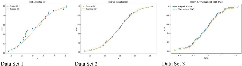
Figure 5 KS plot for the Data Sets 1, 2 & 3 for MOME.

Table 3 Percentage comparison of LBWIs with other distributions

Date Set	Difference of LBWIs with the other Distributions	-2lnL	AIC	AICC	BIC
Data Set 1	Ishita	3.199684	3.173293	3.172327	3.153089
	Akash	0.083098	0.082413	0.082366	0.08193
	Lindley	5.236633	5.195718	5.192878	5.166854
	Exponential	7.482151	7.428034	7.424275	7.389818
Data Set 2	Ishita	2.534732	2.512215	2.511679	1.579892
	Akash	0.503857	0.499403	0.499271	0.49453
	Lindley	5.919121	5.869873	5.868408	5.815919
	Exponential	8.886596	8.853752	8.851738	8.779516
Data Set 3	LBT	0.124663	0.123748	0.85393	0.6128
	Tornumonkpe	5.259663	5.223074	5.185603	5.221801
	Exponential	17.78845	17.6866	17.58204	17.68305

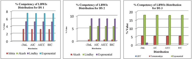
Figure 6 Percentage comparison of LBWIs with other distributions.

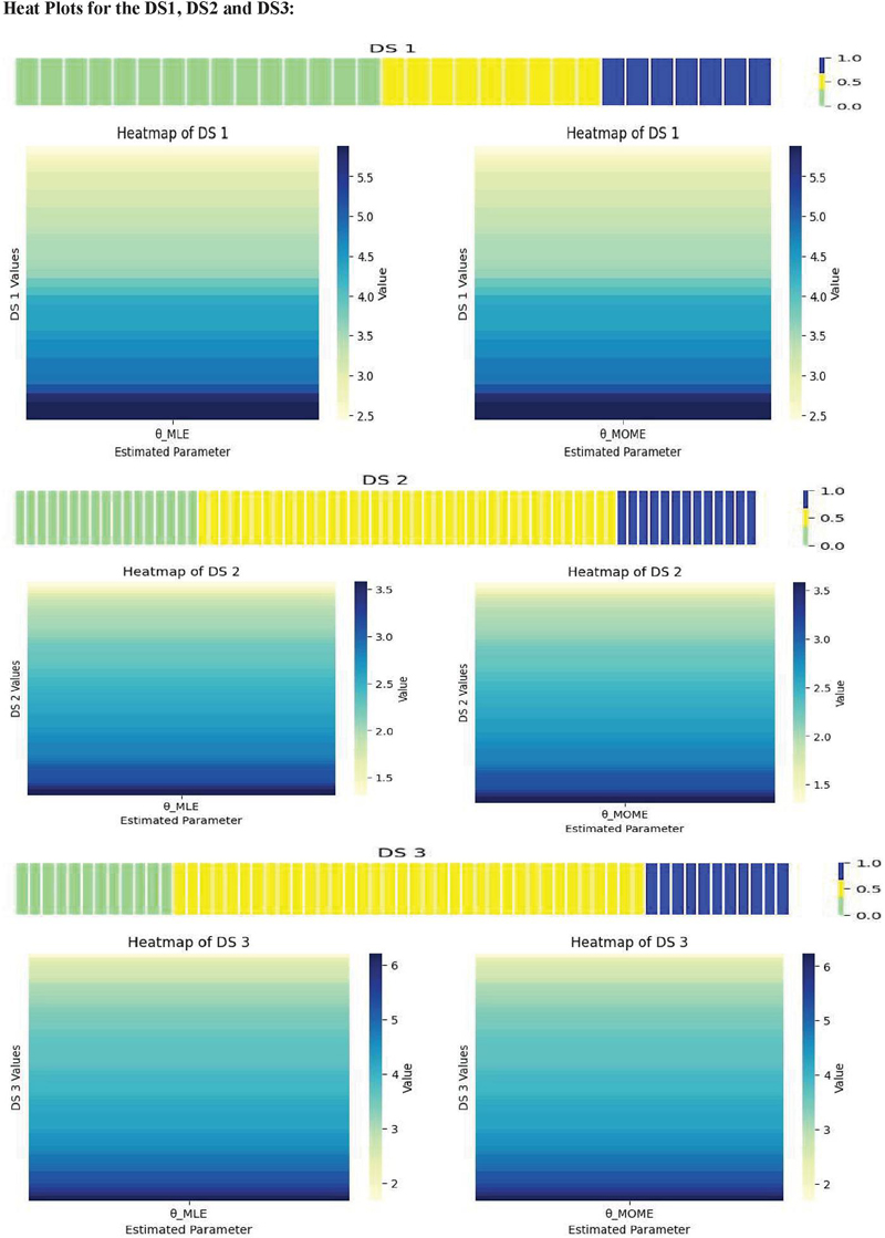
Figure 7 Heat map plot for the DS1, DS2 & DS3 for the estimated value of $θ$ through the MLE and MOME.

6 Reliability Analysis of the Data Set 1(DS 1) and Data Set 3 (DS 3)

Though the estimation of the parameter ( $\hat{θ}$ ) and numerical findings of the MLE of $\hat{θ}$ , S.E. $\hat{θ}$ , -2ln L, AIC, AICC, and BIC provided statistically significant evidence to demonstrate the competency of the proposed Length Biased Weighted Ishita distribution (LBWIs), we performed additional analysis to validate the superiority of our proposed model over existing distributions like Ishita, Akash, Lindley, and exponential distributions. The following table (Table 1) and Figure 4 show the values of the reliability function for the Ishita, Akash, Lindley, exponential, and Length Biased Weighted Ishita (LBWIs) distributions for the estimated values of $\hat{θ}$ , as given in Table 1 for DS 1 and DS 3. Due to some valid and technical reasons, we have avoided the estimation of the reliability function for Dataset 2 (DS 2).

Table 4

DS1
LBWIs	Ishita	Akash	Lindley	Exponential
0.756429626	0.721736225	0.72036797	0.646119706	0.543300883
0.748575346	0.669976218	0.66882239	0.602196441	0.509706607
0.747144723	0.647438325	0.646378246	0.583524359	0.49574837
0.747125451	0.611557238	0.610645362	0.554242066	0.474178237
0.747340456	0.606367265	0.605476644	0.550045591	0.471115496
0.748758073	0.5852178	0.584413153	0.53303243	0.458763707
0.749407713	0.578279504	0.577502807	0.527479302	0.454753211
0.753195607	0.548443392	0.547785186	0.50373552	0.437709426
0.753272572	0.547942606	0.547286363	0.503338676	0.437425882
0.754391864	0.540951765	0.540322829	0.497803988	0.4334755
0.75844057	0.518994071	0.518449658	0.480476422	0.421154302
0.75883899	0.517040948	0.516503956	0.478938834	0.420064083
0.758889173	0.516797055	0.516260989	0.478746868	0.419928005
0.760275574	0.510232984	0.509721731	0.473583427	0.416270496
0.763678238	0.495317861	0.494862262	0.461870708	0.407991883
0.778039798	0.443642238	0.443370769	0.421426793	0.379553393
0.786902355	0.416997845	0.416815357	0.400597322	0.364961285
0.803335627	0.373449862	0.37340272	0.366471914	0.341065752
0.807650228	0.3629187	0.362902231	0.358189008	0.33525897
0.80789563	0.362328868	0.362314092	0.357724622	0.334933257
0.808960318	0.35978071	0.359773217	0.355717787	0.333525485
0.816128289	0.343053793	0.343092819	0.342516879	0.324255336
0.824333849	0.324711464	0.32479883	0.327976912	0.314019561
0.825660937	0.321816174	0.321910904	0.325674722	0.312395895
0.834514429	0.302946903	0.303087762	0.31061619	0.301751333
0.835338571	0.301227112	0.30137201	0.309238622	0.300775241
0.835420944	0.301055543	0.301200842	0.309101143	0.300677806
0.855574632	0.260627124	0.260858756	0.276416377	0.27737303
0.888727699	0.199085376	0.199412304	0.225142511	0.240014006
0.897071447	0.184266214	0.18460841	0.212412439	0.230524991
0.897664405	0.183220743	0.18356389	0.211507334	0.229846312

Table 5

DS3
LBWIs	Lindley	Exponential
0.625610139	0.74625462	0.650917386
0.545704713	0.637068038	0.552834035
0.539815601	0.623051748	0.541002799
0.532525064	0.600800764	0.522492413
0.528971419	0.585564917	0.509993645
0.528867209	0.58502778	0.50955544
0.52545963	0.558255222	0.487908858
0.525832859	0.526383099	0.462586298
0.526253411	0.521935819	0.459087102
0.526481339	0.51984634	0.457445737
0.527961198	0.509067548	0.449004765
0.528671873	0.504878903	0.445736006
0.531479992	0.491322724	0.435198042
0.533836804	0.482051862	0.428025243
0.536355283	0.473371805	0.421332687
0.537285863	0.470398566	0.419045116
0.537686652	0.46915058	0.418085648
0.538763447	0.465885642	0.415577483
0.545042074	0.448819086	0.402510199
0.545556854	0.447536673	0.40153106
0.548904265	0.439525814	0.395422682
0.549420137	0.438336957	0.394517301
0.550168408	0.436632096	0.393219446
0.550397692	0.43611419	0.392825295
0.55092445	0.434932096	0.391925861
0.551821687	0.43294265	0.390412733
0.552089515	0.432354472	0.389965522
0.557340948	0.421291002	0.381565176
0.562575424	0.411006087	0.373773936
0.564596235	0.407198478	0.370893412
0.56554167	0.405444787	0.369567365
0.565845487	0.40488482	0.369144031
0.565921537	0.40474492	0.369038274
0.568452023	0.400148876	0.365565222
0.576342479	0.386465805	0.355239148
0.582073696	0.377039402	0.348135061
0.583431764	0.374859423	0.346493023
0.585956804	0.370855861	0.343478105
0.587205118	0.368899301	0.342004996
0.587455264	0.368508969	0.341711133
0.58749697	0.368443946	0.341662181
0.589461929	0.365398066	0.339369303
0.595363496	0.356443583	0.332630233
0.606198859	0.340646835	0.320743433
0.606541788	0.340158643	0.320376026
0.607785394	0.338393701	0.319047704
0.614052915	0.329620968	0.312443479
0.623314498	0.316984532	0.302922748
0.631665323	0.305867154	0.294534869
0.634163213	0.302584854	0.292055723
0.638207885	0.297307123	0.28806638
0.642891465	0.291247608	0.283480967
0.659990582	0.269495808	0.266964563
0.661423587	0.26769327	0.265591203
0.662810727	0.265950708	0.264262767
0.677233918	0.247930848	0.2504757
0.692789512	0.228573804	0.235544575
0.706225388	0.211773156	0.222457587
0.722960186	0.190521839	0.205689791

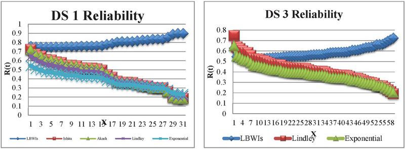
Figure 8 Reliability Plot for the DS1 & DS3.

7 Conclusion

In this paper, we introduce an innovative length-biased distribution, aptly named the Length Biased Weighted Ishita (LBWIS) distribution. This novel approach marks significant advancements in the field, offering a thorough analysis of its statistical and mathematical properties. Key features, including the moment-generating function, characteristic function, cumulant-generating function, and moments, are carefully explored. Additionally, we investigate reliability measures and less commonly estimated functions, such as the Mills ratio, stress-strength reliability, mean deviation about the mean, and mean deviation about the median.

The parameters of the LBWIS distribution are estimated using both the method of moments and maximum likelihood estimation techniques. Additionally, Bayesian estimation is employed to obtain the parameter estimates. To demonstrate its practical applicability, we evaluate the LBWIS distribution against three datasets (DS 1, DS 2, and DS 3), comparing its performance with established distributions, including Ishita, Akash, Exponential, Lindley, Tornumonkpe, and Length Biased Tornumonkpe (LBT).

Our findings, presented in Tables 2, 3, 4, and 5, along with Figures 5, 6, and 8, conclusively demonstrate the superior fit of the LBWIS distribution across all analyzed datasets. Specifically, Table 3 and Figure 6 show that the information criteria values (-2lnL, AIC, AICC, and BIC) for the LBWIS distribution are significantly lower than those for the alternative distributions. This substantial reduction, detailed in the percentage comparison in Table 2, confirms the exceptional fit of the LBWIS distribution for datasets 1, 2, and 3. Table 2 also presents parameter estimates obtained using the method of moments (MOME), while Figure 5 displays the Kolmogorov-Smirnov (KS) plots for these estimated values of $θ$ , further validating the good fit of the LBWIS distribution for DS 1, DS 2, and DS 3. Moreover, Table 1 provides a thorough comparison of the first four moments about the origin ( $μ$ 1 $^{'}$ , $μ$ 2 $^{'}$ , $μ$ 3 $^{'}$ , $μ$ 4 $^{'}$ ) and the mean ( $μ$ 1, $μ$ 2, $μ$ 3, $μ$ 4), alongside measures of skewness ( $β$ 1, $γ$ 1), kurtosis ( $β$ 2, $γ$ 2), and the coefficient of variation (C.V). These comparisons underscore the robustness and reliability of the LBWIS distribution, further confirming its efficacy in fitting the given datasets. Figure 7 separately illustrates the heat plot for DS 1, DS 2, and DS 3.

Thus, the Length Biased Weighted Ishita (LBWIS) distribution demonstrates strong competencies in several key areas. It excels not only in mathematical and statistical properties but also in parameter estimation through both the method of moments and maximum likelihood estimation. Empirical evidence, including lower values for information criteria and better fits in Kolmogorov-Smirnov plots compared to alternative distributions, confirms its superior performance across various datasets. Overall, the LBWIS distribution proves to be a reliable and effective tool for statistical analysis and data fitting when compared to the existing Ishita, Akash, Exponential, Lindley, Tornumonkpe, and Length Biased Tornumonkpe distributions.

7.1 Discussion

This paper introduces the Length Biased Weighted Ishita (LBWIS) distribution, marking a significant advancement in length-biased distributions. We thoroughly explore its statistical properties, including moment generating functions, cumulants, and reliability measures. The LBWIS distribution is evaluated using both the method of moments and maximum likelihood estimation techniques.

Our results, presented in Tables 2, 3, 4, and 5, and Figures 5, 6, 7, and 8, demonstrate that the LBWIS distribution offers a superior fit compared to established distributions such as Ishita, Akash, Exponential, Lindley, Tornumonkpe, and Length Biased Tornumonkpe (LBT). Specifically, the LBWIS distribution exhibits lower values for information criteria (-2lnL, AIC, AICC, and BIC), confirming its better fit across datasets DS 1, DS 2, and DS 3. Kolmogorov-Smirnov plots and parameter estimates further validate its effectiveness. Overall, the LBWIS distribution proves to be a robust and reliable tool for statistical analysis, offering a significant improvement over existing models.

Future Research Scope

Few rarely used techniques and methods can be employed to reshape the proposed LBWIs distribution. However, I personally believe that we should utilize techniques from the non-homogeneous Poisson process, along with considering accelerated scenarios and other relevant approaches.

Funding

This research was conducted without any external funding.

Conflicts of Interest

The authors have no conflicts of interest to disclose.

References

[1] Fisher, R. A. (1934). The effects of methods of ascertainment upon the estimation of frequencies. Annals of Eugenics, 6, 13–25.

[2] Rao, C. R. (1965). On discrete distributions arising out of method of ascertainment, in classical and Contagious Discrete, G.P. Patiled; Pergamum Press and Statistical Publishing Society, Calcutta. 320–332.

[3] Cox, D. R. (1969). Some sampling problems in technology, In New Development in Survey Sampling, Johnson, N. L. and Smith, H., Jr. (eds.) New York Wiley- Interscience, 506–527.

[4] Zelen, M. (1974). Problems in cell kinetic and the early detection of disease, in Reliability and Biometry, F. Proschan and R.J. Sering, eds, SIAM, Philadelphia, 701–706.

[5] Rather, A. A. and Subramanian C. (2018). Characterization and estimation of length biased weighted generalized uniform distribution, International Journal of Scientific Research in Mathematical and Statistical Science, vol. 5, issue 5, pp. 72–76.

[6] Rather, A. A. and Subramanian C. (2018). Length Biased Sushila distribution, Universal Review, vol. 7, issue. XII, pp. 1010–1023.

[7] Rather, A. A. and Ozel G. (2021). A new length-biased power Lindley distribution with properties and its applications, Journal of Statistics and Management Systems, DOI: 10.1080/09720510.2021.1920665.

[8] Rather, A. A. and Subramanian, C. (2019), The Length-Biased Erlang–Truncated Exponential Distribution with Life Time Data, Journal of Information and Computational Sciencse, vol. 9, Issue 8, pp. 340–355.

[9] Rather, A. A., Subramanian, C., Shafi, S., Malik, K. A., Ahmad, P. J., Para, B. A., and Jan, T. R. (2018). A new Size Biased Distribution with applications in Engineering and Medical Science, International Journal of Scientific Research in Mathematical and Statistical Sciences, Vol. 5, Issue 4, pp. 75–85.

[10] Shanker R, Shukla KK. Ishita distribution and its applications. BiomBiostatInt J. 2017;5(2):39–46. DOI: 10.15406/bbij.2017.05.00126.

[11] Shukla, K. K., Shanker, R., and Tiwari, M. K. (2020). Zero-truncated poisson-ishita distribution and its applications. Journal of scientific research, 64(2), 287–294.

[12] Hassan, A., Akhtar, N., Rashid, A., and Iqbal, A. (2021). A New Compound Lifetime Distribution: Ishita Power Series Distribution with Properties and Applications. Journal of Statistics Applications & Probability, 10(3), 883–896.

[13] Ahmad, A., Ahmad, S. P., and Ahmed, A. (2016). Length-biased weighted Lomax distribution: statistical properties and application. Pakistan Journal of Statistics and Operation Research, 245–255.

[14] Saghir, A., Khadim, A., and Lin, Z. (2017). The Maxwell length-biased distribution: Properties and estimation. Journal of Statistical theory and Practice, 11, 26–40.

[15] Rajagopalan, V., Ganaie, R. A., and Rather, A. A. (2019). A New Length biased distribution with Applications. Science, Technology and Development, 8(8), 161–174.

[16] Dey, S., Ali, S., and Kumar, D. (2020). Weighted inverted Weibull distribution: Properties and estimation. Journal of Statistics and Management Systems, 23(5), 843–885. https://doi.org/10.1080/09720510.2019.1669344.

[17] Mansoor, M., Tahir, M., Cordeiro, G., Ali, S. and Alzaatreh, A. (2020). The Lindley negative-binomial distribution: Properties, estimation and applications to lifetime data. MathematicaSlovaca, 70(4), 917–934. https://doi.org/10.1515/ms-2017-0404.

[18] Ali, S., Dey, S., Tahir, M. H., and Mansoor, M. (2021). The Poisson Nadarajah-Haghighi Distribution: Different Methods of Estimation. Journal of Reliability and Statistical Studies, 14(02), 415–450. https://doi.org/10.13052/jrss0974-8024.1423.

[19] Chaito, T., and Khamkong, M. (2021). The length–biased Weibull–Rayleigh distribution for application to hydrological data. Lobachevskii Journal of Mathematics, 42(13), 3253–3265.

[20] Ogunde, A. A., Dutta, S., and Almetawally, E. M. (2024). Half Logistic Generalized Rayleigh Distribution for Modeling Hydrological Data. Annals of Data Science, 1–28.

[21] Chesneau, C., Tomy, L., and Jose, M. (2024). On a New Two-Parameter Weighted Exponential Distribution and Its Application to the COVID-19 and Censored Data. Thailand Statistician, 22(1), 17–30.

[22] Hashempour, M., and Alizadeh, M. (2023). A New Weighted Half-Logistic distribution: Properties, applications and different method of estimations. Statistics, Optimization & Information Computing, 11(3), 554–569.

[23] Roshni, C., Venkatesan, D., and Prasanth, C. B. (2024). A Generalized Area-Biased Power Ishita Distribution Properties and Applications. Indian Journal of Science and Technology, 17(29), 3037–3043.

[24] Ferreira, A. A., and Cordeiro, G. M. (2023). The exponentiated power Ishita distribution: Properties, simulations, regression, and applications. Chilean Journal of Statistics (ChJS), 14(1).

[25] G. P. Patil and J. K. Ord, “On size-biased sampling and related form-invariant weighted distributions,” Sankhya: Indian J. Stat., Ser. B, 48–61 (1976).

[26] K. K. Das and T. D. Roy, “Applicability of length biased weighted generalized Rayleigh distribution,” Adv. Appl. Sci. Res. 2, 320–327 (2011).

[27] K. K. Das and T. D. Roy, “On some length-biased weighted Weibull distribution,” Adv. Appl. Sci. Res. 2, 465–475 (2011).

[28] M. V. Ratnaparkhi and U. V. Naik-Nimbalkar, “The length-biased lognormal distribution and its application in the analysis of data from oil field exploration studies,” J. Mod. Appl. Stat. Methods 11, 255–260 (2012).

[29] A. K. Al-Khadim and A. N. Hussein, “New proposed length biased weighted exponential and Rayleigh distribution with application,” Math. Theory Modelling 4, 2224–2235 (2014).

[30] Bader MG, Priest AM. Statistical aspects of fiber and bundle strength in hybrid composites. In; hayashi T, Kawata K. Umekawa, editors. Progress in Science in Engineering Composites. ICCM–IV Tokyo; 1982:1129–1136.

[31] Fuller EJ, Frieman S, Quinn J, et al. Fracture mechanics approach to the design of glass aircraft windows: A case study. SPIE Proc. 1994;2286:419–430.

[32] Shaked, M., and Shanthikumar, J. G. (1994). Stochastic orders and their applications.

Biographies

Narinder Pushkarna is a Professor in the Department of Statistics, Ramjas College, University of Delhi. He holds M.Sc. (Statistics), M.Phil. and Ph.D. from the Department of Statistics, University of Delhi, India, and brings over three decades of expertise in teaching, research, training, and consultancy in order Statistics and Reliability Modelling. Five research scholars have been awarded Ph.D. under his supervision. He has published research articles in many reputed journals indexed in SCI/WoS/Scopus and etc.

Mustafa is an active & committed researcher serving as a Research Scholar at the Department of Statistics within the University of Delhi, Delhi, India. He received his M.Sc. degree in Statistics from Bareilly College, Bareilly, Rohilkhand University, Bareilly, Uttar Pradesh, India. His research interest includes reliability modelling and Survival Analysis.

Journal of Reliability and Statistical Studies, Vol. 18, Issue 1 (2025), 213–242.
doi: 10.13052/jrss0974-8024.1819
© 2025 River Publishers