Dynamic Reliability Measures of Multi-state k-out-of-n Systems Using ${\mathit{\text{L}}}_{\mathit{\text{z}}}$-transform

Vaibhav Bisht and S. B. Singh^∗

Department of Mathematics, Statistics and Computer Science, G.B. Pant University of Agriculture and Technology, Pantnagar, India
E-mail: bishtvickybng@gmail.com; drsurajbsingh@yahoo.com
*Corresponding Author

Received 18 December 2024; Accepted 05 March 2025

Abstract

In system engineering, k-out-of-n multi-state system is one of the important systems as it finds wide application in many complex engineering structures. In earlier studies, k-out-of-n multi-state systems were usually thought to be operated in non dynamic state. However, in reality, these systems can have components whose states change over time, making them dynamic in nature. To tackle this, we propose a method utilizing the $L_z$-transform to obtain the dynamic reliability measures of such systems. The system’s components are presumptively Markov-process compliant and are only repaired after a total failure. In the proposed research work the reliability, availability, instantaneous performance expected, and deficiency in performance are found for the system under consideration. Lastly, a real-life example of the oil supply system is investigated to authenticate the proposed approach. It was observed that the reliability and availability of the oil supply system decline as the minimum number of required components in different states increases.

Keywords: $L_z$-transform, reliability, availability, and universal generating function.

Notations

M	The state of the complete performance of the system
$g_{ij}$	The performance level of component i which is in state j
${\lambda }_{jk}^i$	Transition (failure) rate of component i from state j to state k (j $>$ k)
${\mu }_{jk}^i$	Transition (repair) rate of component i from state j to state k (j $<$ k)
k	The minimum number of components required for working of
	k-out-of-n system
$R(t)$	Reliability of k-out-of-n system at any instant t
$A(t)$	Availability of k-out-of-n system at any instant t.

1 Introduction

The reliability theory is basically ashore on the fundamental task of obtaining the reliability indices of various engineering systems. The system could either be a binary system or a multi-state system (MSS). In contrast to the multi-state system, which has a finite number of states or performance levels, the binary system only has two states: the fully operational state and the state of failure. The majority of complex engineering systems have several states with varying performance levels. Due to its use in engineering structures, reliability analysis of MSS has been a topic of research since the late 1970s [1, 5]. Since then, it has drawn the interest of numerous researchers and engineers. Lisnianski and Levitin [17] summarized the theory of multi-state system reliability. There are several well-known MSS systems, including parallel, series, k-out-of-n, bridge, etc. The k-out-of-n (k/n) system is one of the most significant systems since it is utilized in a wide range of applications, including spacecraft, traffic control systems, communication networks, and weapon systems [11, 12].

A k/n:G system works if the minimum of its k elements are operative, as opposed to a k/n:F system which becomes non-functional only when all k components cease to operate. For instance, the typical message load in a communication system with 10 transmitters would demand that at least 8 of them be operational, failing which some messages might be lost. As a result, this transmission system operates at an 8/10:G system. El-Neweihi et al. [5] introduced the first multi-state k/n system model. The multi-state k/n system model was also defined by Boedigheimer and Kapur [4] with the aid of the lower and higher boundary points, and their definition was in agreement with that of El-Neweihi et al. Numerous research have been done in the past in the field of the k/n systems [6, 9, 20, 24, 25, 28]. Further, a variety of methods have been used to find the reliability of the $k/n$ system including stochastic process approach, the universal generating function method (UGF), and the Monte Carlo simulation technique. Among these various techniques, the UGF approach has been widely used because of its simplicity and efficiency in reducing computational time.

The UGF method is employed to determine the performance distribution of a MSS by utilizing the performance characteristics of its individual components through straightforward arithmetic computations. This approach, pioneered by Ushakov [21], has since become a commonly utilized method among reliability scientist for analyzing system reliability [13, 18, 19, 23, 29] and network reliability [2, 3, 10, 22]. The foremost drawback of the vital method is such, preferably, it is only applicable to the random variables; hence, when evaluating the reliability of the multi-state systems, it is only applicable to performance distributions of the states that are steady. Resultantly, in the present circumstances, it is not possible to calculate transient approaches in the MSS, aging MSS, and MSS under increasing or decreasing stochastic demand incorporating the elementary universal generating function (UGF) techniques. To extend the application of the UGF technique in the reliability assessment of the multi-state system in a dynamic state, where the entire structure and its components be defined by stochastic processes, the $L_z$-transform [14] was formulated for Markov process with states taken to be discrete and time to be continuous (DSCT markov process). Thus, the $L_z$-transform can be viewed as an extension of the universal generating function (UGF) approach for analyzing stochastic processes. The $L_z$-transform has been applied in various research efforts to evaluate the time-dependent reliability of engineering systems. For example, Frenkel et al. [7] explored the cooling efficiency of a deteriorating multi-state cooling system in MRI devices using this technique. Lisnianski and Benhaim [15] obtained the reliability indices of the power station by the $L_z$-transform. Frenkel et al. [8] assessed the critical aspects of the vehicle’s operational sustainability, such as its availability, power output, and power output deficit in the Norilsk icebreaker ships’ multi-state multi-power source traction drive by the $L_z$-transform. The book [16] provided theoretical insights, practical applications, and case studies drawn from real-world experiences in the field of time-dependent reliability analysis of MSSs. Bisht and Singh [25] obtained the dynamic reliability measures of weighted K/n system with the help of $L_z$-transform. Lisnianski et al. [31] published an article on sensitivity analysis of aging multi-state system by using $L_z$-transform method. Bisht and Singh [26] extended the conventional $L_z$-transform to Interval $L_z$-transform ($I{L}_z$), to evaluate the reliability indices of MSS, even in cases where data is incomplete or uncertain. Singh et al. [27] introduced an algorithm using the $L_z$-transform to assess reliability indices in dynamic multi-state m-out-of-r-within-$k/n$ systems, accounting for time-varying component states and Markov processes. Bo et al. [30] proposed a novel approach combining the $L_z$-transform and deep neural networks (DNN) to evaluate the reliability of series-parallel systems governed by a semi-Markov process.

In many complex engineering systems, the state of the system evolves over time, meaning the probabilities associated with different states of multi-state components change dynamically. This paper aims to apply the $L_z$-transform to better analyze and understand $k/n$ system, which are systems that function as long as at least k out of n components are operational. The focus is on addressing failures of varying severities, from minor issues to critical breakdowns, as well as significant repair activities in such dynamic environments. The proposed approach introduces a novel and efficient method to determine the dynamic reliability indices of k/n multi-state systems (MSS), which are composed of components capable of multiple performance levels. The rest of this paper is structured as follows: Section 2 discusses the description of multi-state $k/n$ system. Third section gives light on elementary definition and the properties of $L_z$-transform. Section 4 presents an step wise step method to obtain the dynamic reliability indices of the $k/n$ multi-state system. In Section 5, a real life example of the oil supply system demonstrates the suggested algorithm’s validity, and the results are addressed in Section 6.

2 System Description

Let us examine a multi-state system consisting of $n$ elements, each capable of functioning in multiple states, structured in a $k/n$ configuration. The state space of each component and the system is represented by the set $\{1,2,\mathrm{\dots },M-1,M\}$ and the states of the components entirely determine the state of the system. State M represents the ideal state of operation, state 1 the ideal state of total failure, and all other states are intermediate states. It is assumed that the components are fixed only when it is at state 1, so it transfers to perfect functioning state i.e., to state M. The state of the component can change with respect to time i.e., the state M is transitioned to lower states $M-1$, $M-2$ etc. and at the state 1, the component is again transitioned to state M. In major failure the element is transitioned from state i to state j such that $j<i-1$ and minor failure causes the component transition from state i to $i+1,1\le i,j\le M$. In contrast to the major repair, which returns an element from state j to state i when $i>j+1$, the minor repair returns an element from state j to state $j+1$; $1\le i,j\le M$. Hence, the dynamic characteristics of the multi-state $k/n$ system with minor and major failure and major repair are studied extensively in this paper.

3 ${\mathit{\text{L}}}_{\mathit{\text{z}}}$-transform

Consider a DSCT Markov process, represented as $G(t)=\{g,\mathrm{A},p_0\}$. This process has M probable states, with g representing the set of these states, defined as the set $G(t)\in \{g_{i1},g_{i2},\mathrm{\dots },g_{iM}\}$; $\mathbf{\text{A}}=[a_{ij}(t)]$, $i,j=1,2,\mathrm{\dots }M$ is the matrix representing transitions and $p_0$ is the probability distribution of the starting state and is given by

$$p_0=[p_{i0}=\mathrm{Prob}\{G(0)=g_i\},\mathrm{\dots },p_{k0}=\mathrm{Prob}\{G(0)=g_k\}]$$

Subsequently, the $L_z$-transform applied to a Markov process $G(t)=\{g,\mathrm{A},p_0\}$, where $g$ represents the set of states $G(t)\in \{g_{i1},g_{i2},\mathrm{\dots },g_{iM}\}$ for $t\ge 0$, $\mathit{\text{A}}=[a_{ij}(t)]$ is the transition intensity matrix with j ranging from 1 to M and $p_0$ is the initial state probability distribution $p_0$ is given by

$$L_z(G(t))=f(z,t,p_0)=\sum _{j=1}^M{p}_{ij}(t)z^{g_{ij}}$$

(1)

It is crucial to understand that the $L_z$-transform is distinct from a UGF, as it is a fundamentally different entity that depends on the initial conditions of the Markov process $p_0$ and the time t. The property, which shall be used in computation, is as follows.

Property 1: UGF operator “${\mathrm{\Omega }}_f$” to $L_z$-transform in $M(t)$ and $N(t)$ for $t\ge 0$ can be used to generate the $L_z$-transform from two separate Markov processes, $f(M(t),N(t))$.

$$L_z\{f(M(t),N(t)\}={\mathrm{\Omega }}_f(L_z\{M(t)\},L_z\{N(t)\})$$

(2)

4 Algorithm for Computing Dynamic (Time-Dependent) Reliability Indices of k/n System by ${\mathit{\text{L}}}_{\mathit{\text{z}}}$-transform

Consider a repairable $k/n$ MSS which has n multistate components, each of which has M distinct performing states ranging from $1,2,3,\mathrm{\dots },M$. In this case, the states between M, the greatest performing state, and 1, the state of failure represent intermediate states. Assume that each element of the $k/n$ MSS degrades according to the Markov process. A repairable component’s Markov model, or state transition diagram, is shown in Figure 1 along with M different performance stages, as well as major and minor failure and repair. In Figure 1, ${\lambda }_{M,M-1}^{(i)}$ represents the minor failure which is a malfunction or failure of a system or component that, while not causing catastrophic or severe consequences, still influences performance or operation to some extent and ${\lambda }_{M,1}^{(i)}$ and ${\mu }_{1,M}^{(i)}$ are the major failure and major repair for component $i$ respectively. The major failures have a profound impact on the performance, functionality, and overall reliability of the system. These failures stem from various factors, including inadequate maintenance, material defects, human error, fatigue, overload, and more.

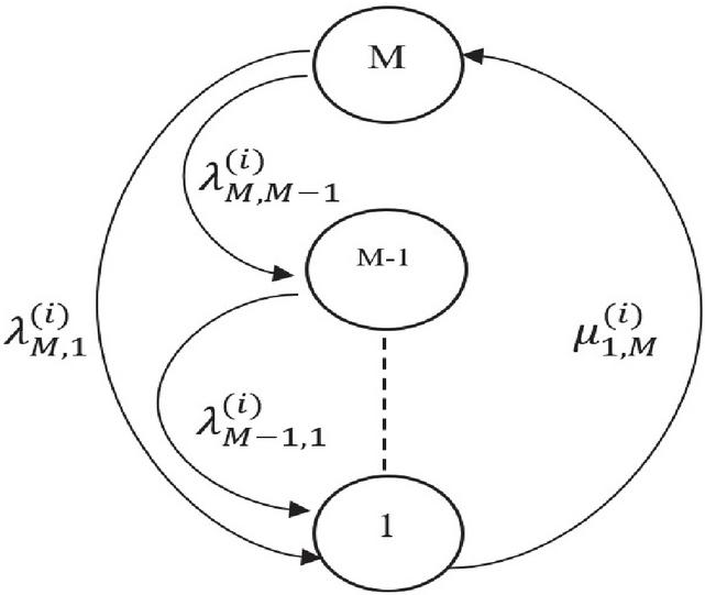
Figure 1 State transition diagram.

4.1 ${\mathit{\text{L}}}_{\mathit{\text{z}}}$-transform of Multi-state Element

Obtaining the $L_z$-transform of each element is the first step in computing the dynamic reliability indices of a repairable $k/n$ MSS. In order to calculate it, firstly, obtain the states’ set represented by, $g=\{g_{i1},g_{i2},\mathrm{\dots },g_{iM}\}$, where $g_{ij}$ is the performance levels of component i, which i in state j, $j=1,2,\mathrm{\dots },M$. Now, the time function of probability distribution of component i in state j i.e., $p_{ij}(t)$ can be obtained by solving simultaneously the system of differential Equation (3) with the help of initial conditions $p_{iM}(0)=1,\mathrm{\dots },p_{i2}(0)=0,p_{i1}(0)=0$.

$$\begin{array}{c}\frac{d{p}_{iM}(t)}{dt}=\sum _{e=1}^{M-1}{\mu }_{eM}^{(i)}\cdot p_{ie}(t)-p_{iM}(t)\sum _{e=1}^{M-1}{\lambda }_{e{M}_i}^{(i)}\hfill \\ \frac{d{p}_{ij}(t)}{dt}=\sum _{e=j+1}^M{\lambda }_{ej}^{(i)}\cdot p_{ie}(t)+\sum _{e=1}^{j-1}{\mu }_{ej}^{(i)}.p_{ie}(t)\hfill \\ -p_{ij}(t)\left(\sum _{e=1}^{j-1}{\lambda }_{je}^{(i)}+\sum _{e=1}^M{\mu }_{je}^{(i)}\right)\hfill \\ \frac{d{p}_{i1}(t)}{dt}=\sum _{e=2}^M{\lambda }_{e1}^{(i)}\cdot p_{ie}(t)-p_{i1}(t)\sum _{e=2}^M{\mu }_{ie}^{(i)}\hfill \end{array}\}$$

(3)

In Equation (3), $\frac{d{p}_{iM}(t)}{dt}$ represents how fast the probability changes for component i to be in its highest state, $M$. On the other hand, $\frac{d{p}_{ij}(t)}{dt}$ indicates the rate at which the probability changes for component i to be in state j, where j ranges from 1 to $M-1$. These terms are crucial for monitoring how the system’s state probabilities evolve over time. The transition rates $\lambda$ and $\mu$, which describe the likelihood of moving between different states, are key factors influencing these equations.

The $L_z$-transform of one element i can be obtained subsequently as:

$$L_z(G_i(t))=\sum _{j=1}^M{p}_{ij}(t)z^{g_{ij}}$$

Once one element’s $L_z$-transform has been determined, a similar procedure may be used to determine the $L_z$-transform for each of the $k/n$ system’s component i.

4.2 ${\mathit{\text{L}}}_{\mathit{\text{z}}}$-transform of Multi-state $k/n$ System

The $L_z$-transform of entire multi-state $k/n$ system can be obtained by operating UGF operator ${\mathrm{\Omega }}_f$ on the $L_z$-transform of multi-state elements, as shown in the Property 1. Let $L_z(G_1(t)),L_z(G_2(t))\mathrm{\dots },L_z(G_n(t))$ be the $L_z$-transform of 1st, 2nd and $n$th element correspondingly, i.e.,

$$L_z(G_i(t))=\sum _{j=1}^M{p}_{ij}(t)z^{g_{ij}},i=1,2,\mathrm{\dots }n.$$

Then, $L_z$-transform corresponding to entire complex $k/n$ MSS is obtained as:

$L_z(G_{sys}(t))$	$={\mathrm{\Omega }}_{k\text{-out-of-}n}(L_z(G_1(t)),L_z(G_2(t)),\mathrm{\dots }$
	$\mathrm{\hspace{1em}\hspace{1em}}{L}_z(G_{n-1}(t)),L_z(G_n(t)))$
	$={\displaystyle \sum _{j_1=1}^M}{\displaystyle \sum _{j_2=1}^M}\mathrm{\dots }{\displaystyle \sum _{j_{n-1}=0}^M}{\displaystyle \sum _{j_n=0}^M}$
	$\mathrm{\hspace{1em}}\times \left({\displaystyle \prod _{i=1}^n}{p}_{i{j}_i}(t)z^{{\mathrm{\Phi }}_{k\text{-out-of-}n}(g_{i{j}_1},g_{i{j}_2},\mathrm{\dots }{g}_{i{j}_{n-1}},g_{i{j}_n})}\right)$

where $\mathrm{\Phi }(g_{i{j}_i})$ is known as the system’s structure function and it hinge on the topology of the structure (system). The structure function for $k/n$ MSS, when individual component has numerous states is given to be:

$${\mathrm{\Phi }}_{k\text{-out-of-}n}(g_{i{j}_1},g_{i{j}_2},\mathrm{\dots },g_{i{j}_{n-1}},g_{i{j}_n})=\sum _{i=1}^n{g}_{i{j}_i}$$

Following the acquisition of the $L_z$-transform for the entire $k/n$ multistate system, reliability measures can be computed as follows:

4.2.1 Reliability

It is the likelihood that any system will serve its aim for a predetermined period of time in specific operating conditions. With the required number of element k, the $L_z$-transform yields the reliability of the $k/n$ system as

$$R(t)=\sum _{j=1}^M{p}_{ij}(t)\beta ({\mathrm{\Phi }}_{k\text{-out-of-}n}(g_{i{j}_1},g_{i{j}_2},\mathrm{\dots },g_{i{j}_{n-1}},g_{i{j}_n})-k)$$

where,

$$\beta (a)=\{\begin{array}{cc}1,\hfill & a\ge 0\hfill \\ 0,\hfill & a<0\hfill \end{array}$$

4.2.2 Availability

The availability $A(t)$ of the $k/n$ system at any time $t$ for minimum number of required component $k$ can be obtained as

$$A(t)=\sum _{j=1}^M{p}_{ij}(t)\beta ({\mathrm{\Phi }}_{k\text{-out-of-}n}(g_{i{j}_1},g_{i{j}_2},\mathrm{\dots },g_{i{j}_{n-1}},g_{i{j}_n})-k)$$

One can observe that the mathematical representations of the system’s reliability and availability are identical but individually are not exactly same. This is due to the failure rate being taken into account when estimating availability, but not while estimating reliability.

4.2.3 Mean expected performance

The $k/n$ multi-state repairable system’s mean expected performance at time $t\ge 0$ is calculated as

$$E(t)=\sum _{\begin{array}{c}j=1\\ g_{ij}>0\end{array}}^M{p}_{ij}(t)g_{ij}$$

(4)

4.2.4 Mean performance deficiency

The performance shortfall of a $k/n$ multi-state system at any specific time t is calculated from

$$D(t)=\sum _{j=1}^M{p}_{ij}(t)\max (k-g_{ij},0)$$

(5)

5 A Numerical Example: An Oil Supply System

To apply the derived results in the proposed work let us take the oil supply system depicted in Figure 2. Four oil pipelines transport oil from the oil source to three stations then n equals 4. A pipeline is regarded as a multi-state component and any point along a pipeline could experience a failure. Pipeline 1, 2 and 3 have four states and pipeline 4 has 3 states. There are different demands for oil at each station. For Station 1 to operate at full capacity, minimum four pipelines must be operational, $k_1=4$. Station 2 needs at least two pipelines to be operational ($k_2=2$) and Station 3 needs at least three pipelines to function ($k_3=3$). According to the aforesaid descriptions above, this system may be thought of as a $k/n$:G MSS with $n=4$ and $k_1=4$, $k_2=2$, and $k_3=3$. The state of the pipeline changes with time. The pipeline 1, 2 and 3 has four states and pipeline 4 consists of 3 states; therefore, let states 4, 3, 2 and 1 represent these states. For first three pipelines, state 1 is considered to be a total failure condition, while states 2 and 3 are intermediate states. State 4 denotes a perfect functioning state. For pipeline 4, state 3 is perfect operational state, state 2 is intermediate state and state 3 is the state of failure. Let us assume that the pipelines are repaired when it is at lowest state i.e., at state 1, in order to transmit it to perfect operational state. Table 1 signifies the states’ transition rates and the performance of the each four pipelines as:

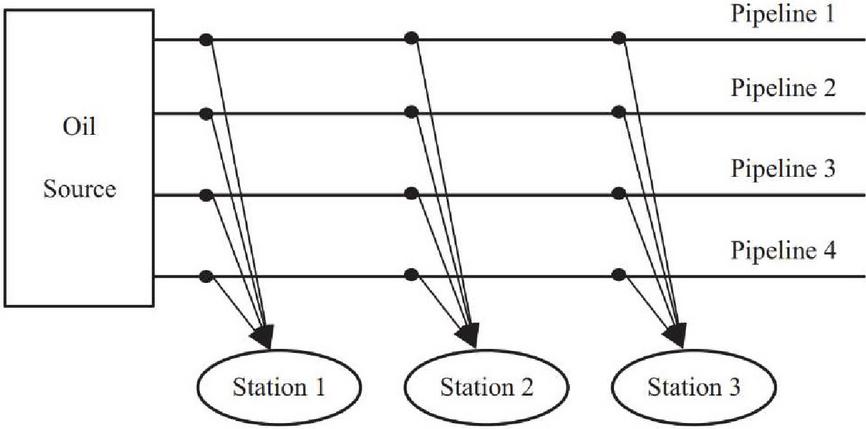
Figure 2 The oil supply system.

Table 1 Pipelines’ performance and transition rates of oil supply system

Oil Supply System	Transition Rates (1/year)
Pipeline	States	S1	S2	S3	S4	Performance Rates
1	S1	0.0	0.0	0.0	4.2	0
	S2	0.3	0.0	0.0	0.0	1.1
	S3	0.5	0.9	0.0	0.0	1.7
	S4	0.7	1.3	2.0	0.0	2.3
2	S1	0.0	0.0	0.0	5.4	0
	S2	0.5	0.0	0.0	0.0	1.6
	S3	0.7	1.2	0.0	0.0	2.0
	S4	0.9	1.6	2.2	0.0	2.8
3	S1	0.0	0.0	0.0	7.2	0
	S2	0.2	0.0	0.0	0.0	0.8
	S3	0.4	0.8	0.0	0.0	1.0
	S4	0.8	1.1	1.8	0.0	1.3
4	S1	0.0	0.0	3.4	–	0
	S2	0.5	0.0	0.0	–	0.9
	S3	0.2	0.8	0.0	–	1.5

Primarily at time $t=0,p_{i4}(0)=1$ for $i=1,2$ and 3; $p_{i3}(0)=1$ for $i=4$ and $p_{ij}(0)=0$ for remaining values of i and j, $1\le i\le 4$, $1\le j\le 4$. Now for this k-out-of-4 system, the set of governing differential equations (3) of pipeline 1 becomes

$$\begin{array}{c}\frac{d{p}_{11}(t)}{dt}=-4.2p_{11}(t)+0.3p_{12}(t)+0.5p_{13}(t)+0.7p_{14}(t)\hfill \\ \frac{d{p}_{12}(t)}{dt}=0p_{11}(t)-0.3p_{12}(t)+0.9p_{13}(t)+1.3p_{14}(t)\hfill \\ \frac{d{p}_{13}(t)}{dt}=0p_{11}(t)+0p_{12}(t)-1.4p_{13}(t)+2p_{14}(t)\hfill \\ \frac{d{p}_{14}(t)}{dt}=4.2p_{11}(t)+0p_{12}(t)+0p_{13}(t)-4p_{14}(t)\hfill \end{array}\}$$

(6)

State probability for pipeline 1 can be obtained by solving Equation (6) under the preliminary conditions $p_{11}(0)=p_{12}(0)=p_{13}(0)=0$ and $p_{14}(0)=1$, as shown in Figure 3.

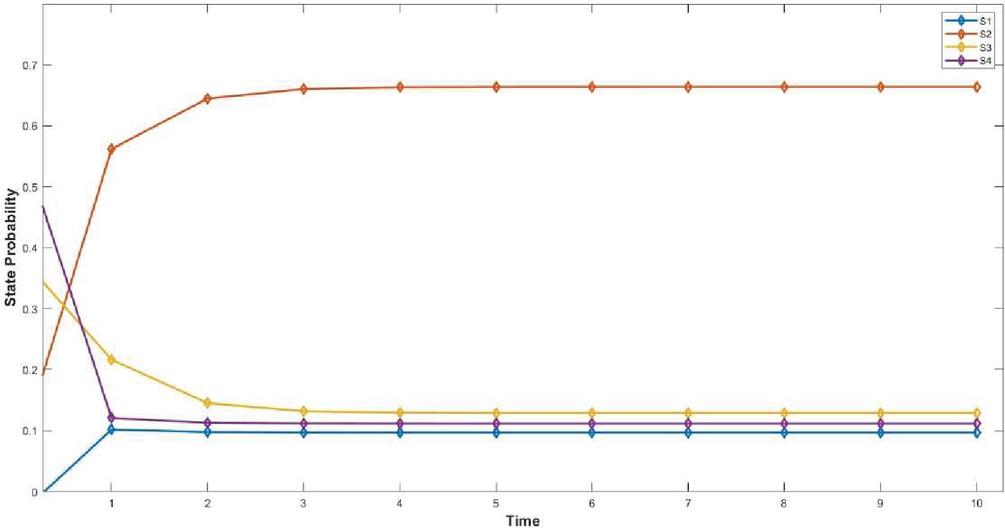
Figure 3 Probability of different states for pipeline-1.

Now, $L_z$-transform for pipeline 1 can be derived using Equation (1) as follows:

$$L_z(G_1(t))=\sum _{j=1}^4{p}_{1j}(t)z^{g_{1j}}=p_{11}{z}^0+p_{12}{z}^{1.1}+p_{13}{z}^{1.7}+p_{14}{z}^{2.3}$$

In a similar manner, the differential equations for the second, third, and fourth pipelines are governed by replacing $i=2,3$ and 4 and changing the value of the states in the Equation (3). By solving these equations in the context of the preliminary conditions, we may get the transient probabilities shown in Figures 4–6 correspondingly.

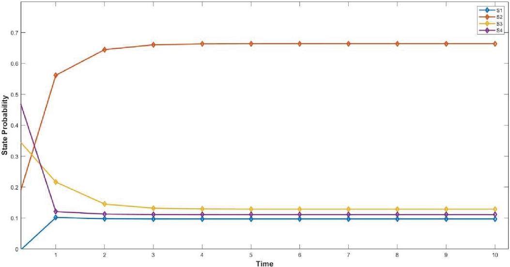
Figure 4 Probability of different states for pipeline-2.

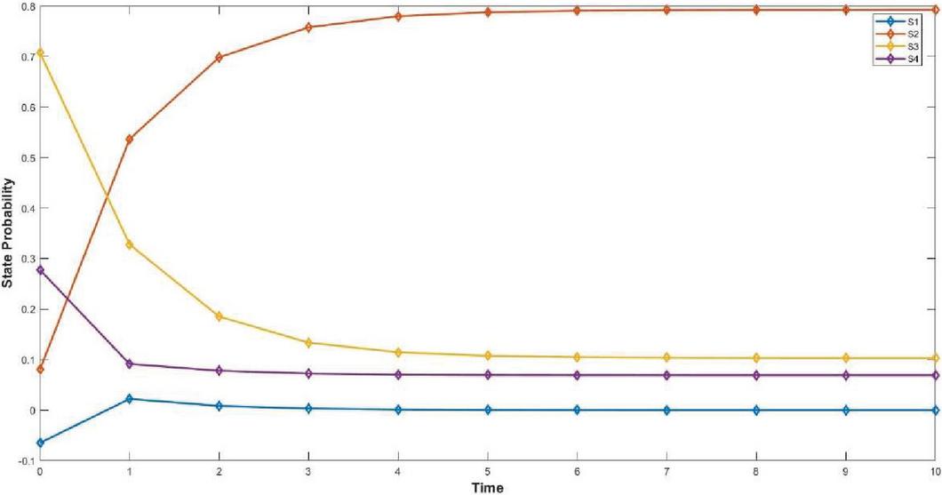
Figure 5 Probability of different states for pipeline-3.

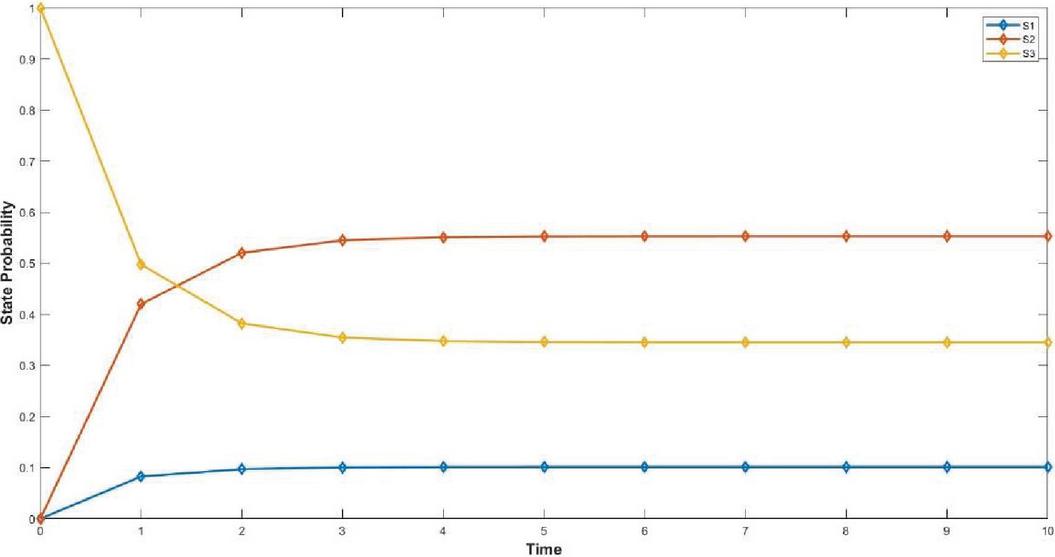
Figure 6 State probability distribution for pipeline-4.

Finally, the $L_z$-transform for pipeline 2, 3 and 4 are found to be:

$L_z(G_2(t))$	$={\displaystyle \sum _{j=1}^4}{p}_{2j}(t)z^{g_{2j}}=p_{21}{z}^0+p_{22}{z}^{1.6}+p_{23}{z}^{2.0}+p_{24}{z}^{2.8}$
$L_z(G_3(t))$	$={\displaystyle \sum _{j=1}^4}{p}_{3j}(t)z^{g_{3j}}=p_{31}{z}^0+p_{32}{z}^{0.8}+p_{33}{z}^{1.0}+p_{34}{z}^{1.3}$
$L_z(G_4(t))$	$={\displaystyle \sum _{j=1}^3}{p}_{4j}(t)z^{g_{4j}}=p_{31}{z}^0+p_{32}{z}^{0.9}+p_{33}{z}^{1.5}$

The $L_z$-transform for the oil supply system consisting of four pipelines, first three having four states and fourth having three states is obtained from Equation (2) and is expressed as

$L_z(G(t))$	$={\mathrm{\Omega }}_{k\text{-out-of-}n}\{L_z(G_1(t)),L_z(G_2(t)),L_z(G_3(t)),L_z(G_4(t))\}$
	$={\mathrm{\Omega }}_{k\text{-out-of-}n}\{(p_{11}{z}^0+p_{12}{z}^{1.1}+p_{13}{z}^{1.7}+p_{14}{z}^{2.3}),$
	$\mathrm{\hspace{1em}\hspace{1em}}(p_{21}{z}^0+p_{22}{z}^{1.6}+p_{23}{z}^{2.0}+p_{24}{z}^{2.8}),$
	$\mathrm{\hspace{1em}\hspace{1em}}(p_{31}{z}^0+p_{32}{z}^{0.8}+p_{33}{z}^{1.0}+p_{34}{z}^{1.3}),$
	$\mathrm{\hspace{1em}\hspace{1em}}(p_{41}{z}^0+p_{42}{z}^{0.9}+p_{43}{z}^{1.5})\}$	(7)

5.1 Reliability

As discussed in the Section 4.2.1, to obtain the reliability, Equation (4) of the pipeline-1 becomes

$\begin{array}{c}{\displaystyle \frac{d{p}_{11}(t)}{dt}}=0.3p_{12}(t)+0.5p_{13}(t)+0.7p_{14}(t)\hfill \\ {\displaystyle \frac{d{p}_{12}(t)}{dt}}=-0.3p_{12}(t)+0.9p_{13}(t)+1.3p_{14}(t)\hfill \\ {\displaystyle \frac{d{p}_{13}(t)}{dt}}=-1.4p_{13}(t)+2p_{14}(t)\hfill \\ {\displaystyle \frac{d{p}_{14}(t)}{dt}}=-4p_{14}(t)\hfill \end{array}\}$

The governing differential equations for pipelines 2, 3 and 4 is obtained in a similar manner toward obtaining the reliability of the oil supply system under consideration by inserting $i=2,3$ and 4 in Equation (3). One can find the state probabilities as depicted in Figures 7, 8, 9 and 10, respectively, by successively solving these equations under the given preliminary conditions.

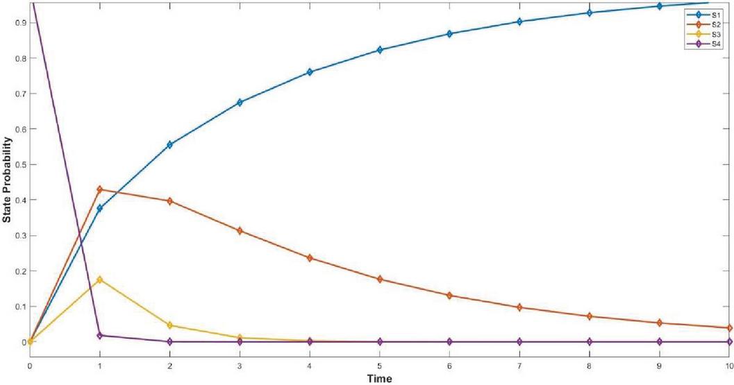
Figure 7 Probability of different states for pipeline-1.

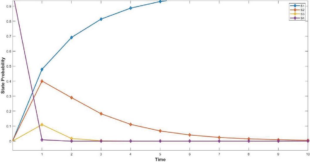
Figure 8 Probability of different states for pipeline-2.

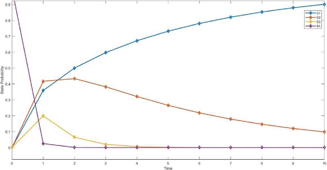
Figure 9 Probability of different states for pipeline-3.

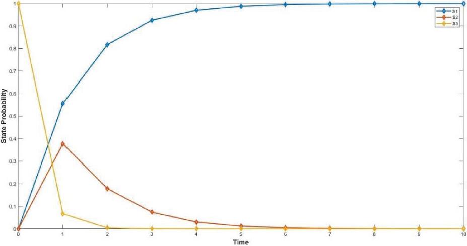
Figure 10 Probability of different states for pipeline-4.

Figures 7–10 illustrate the probabilities of different pipeline states, which are used to determine reliability. To calculate these transient probabilities, the repair rate is set to zero i.e., ${\mu }_{ij}=0\forall i,j$, and the system of differential equations is solved using predefined initial conditions. The results clearly show that the probability increases for the initial states and decreases steadily for the final state, representing the best-performing state. After obtaining the $L_z$-transform of each pipeline according to the determined state probabilities, the $L_z$-transform of the oil supply system is computed through Equation (2). Finally, Equation (5) has been used to determine the reliability of the oil supply system for various minimum needed component counts, i.e., $k_1=4,k_2=2$, and $k_3=3$. Figure 11 depicts a graph that shows the reliability of the system over time and in conjunction with different minimal components. It can be clearly observed that, the reliability decreases over time as the number of minimum required components increase.

Figure 11 Reliability of the oil supply system.

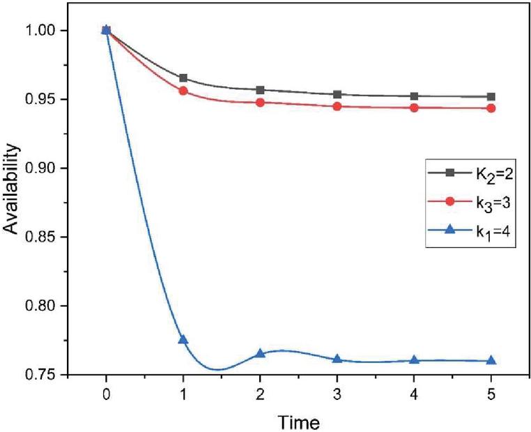
Figure 12 Availability of the oil supply system.

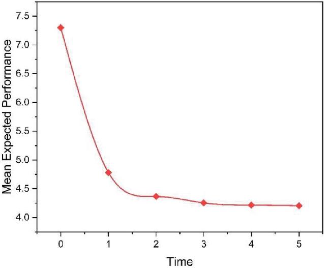
Figure 13 Mean expected performance of the oil supply system.

5.2 Availability

The availability of the oil supply system has been obtained with respect to time and is being plotted in Figure 12 for $k_1=4$, $k_2=2$, and $k_3=3$ respectively. As the minimum required components increase, one can observe a decline in availability over time. It’s noteworthy that availability surpasses reliability at any given time, owing to repair activities.

5.3 Mean Expected Performance

The average expected performance of oil supply system can be calculated from Equation (4). The result obtained is shown in Figure 13 and is evident that the performance expected from the system decrease continuously over time.

5.4 Mean Performance Deficiency

Figure 14 illustrates the average performance deficit of the oil supply system based on the requisite performance $k_1=4,k_2=2$, and $k_3=3$ respectively.

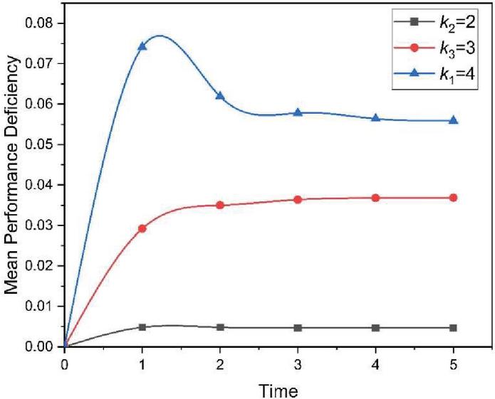
Figure 14 Mean performance deficiency of oil supply system.

6 Conclusion

In this study, the $L_z$-transform has been extensively used to study a multi-state $k/n$ system with major and minor failures as well as substantial repair. The $k/n$ system is of great importance especially in the complex engineering system. The state of the components in the majority of engineering systems changes over time, i.e., the state probabilities of each component are not constant but rather depend on the passage of time. This aspect has been taken into account in this recent $L_z$-transform research. For the $k/n$ multi-state system under consideration, where state probabilities are treated as time-dependent, an algorithm based on the $L_z$-transform is proposed to evaluate time-dependent reliability measures. To validate the suggested algorithm, a case study of an oil supply system is examined. For this system, the reliability measures are calculated in a dynamic context and are plotted for different values of time and minimum number of required component. It can be clearly observed that the reliability and availability of the oil supply system decreases as the number of minimum required component at different states increase. One can easily visualize that for each k, both reliability and availability decline over time in a progressive manner, however, the rate at which dynamic reliability declines is greater than that of dynamic availability. This study bridges theory and practice by offering a dynamic method to evaluate system reliability over time using the $L_z$-transform. Practically, it helps engineers optimize maintenance and resource planning for complex systems. Theoretically, it enhances reliability analysis by incorporating time-dependent state probabilities. This approach ensures better performance insights for real-world applications.

This research provides insights into how the state probabilities of system components change over time, which is crucial for accurately assessing the performance of complex engineering systems. By incorporating the $L_z$-transform, the study offers a robust method to determine the reliability and availability of systems, which are key metrics for system performance and maintenance planning. This study provides valuable insights for operations managers and technical professionals to obtain the system performance in situations where the state probability of system components is time dependent. This study introduces a novel approach to analyzing multi-state k/n systems with time-dependent state probabilities, addressing a critical gap in reliability assessment. The proposed methodology offers a foundation for extending dynamic reliability analysis to diverse and complex engineering systems. This paper does not extend for the case of inspection and maintenance strategies. In future, this methodology can be extended to a wide range of complex engineering systems beyond the k/n systems like, sliding window system, weighted voting system etc., allowing for broader application and further refinement of the algorithm to enhance its accuracy and usability in diverse scenarios.

Acknowledgement

The Department of Science and Technology (India), which provided the first author with an Inspire fellowship (IF 210271) and funding for the work, is warmly acknowledged.

Competing Interests

The authors declare that they have no conflict of interest.

Data Availability Statement

No specific data has been used in the preparation of manuscript.

Credit Authorship Contribution Statement

Vaibhav Bisht: Conceptualization, Methodology, Validation, Formal analysis, Investigation, Writing – original draft.

S. B. Singh: Conceptualization, Methodology, Investigation, Reviewing, Supervision.

References

[1] Barlow, R. E., and Wu, A. S. (1978). Coherent systems with multi-state components. Mathematics of operations research, 3(4), 275–281.

[2] Bisht, V., and Singh, S. B. (2022). Reliability Analysis of 8 $\times$ 8 SEN – Using UGF Method. In: Ram, M., Pham, H. (eds) Reliability and Maintainability Assessment of Industrial Systems. Springer Series in Reliability Engineering. Springer, Cham.

[3] Bisht, V., and Singh, S. B. (2021). Reliability Estimation of 4 $\times$ 4 SENs Using UGF Method. Journal of Reliability and Statistical Studies, 14(1), 173–198.

[4] Boedigheimer, R. A., and Kapur, K. C. (1994). Customer-driven reliability models for multistate coherent systems. IEEE Transactions on reliability, 43(1), 46–50.

[5] El-Neweihi, E., Proschan, F., and Sethuraman, J. (1978). Multistate coherent systems. Journal of Applied Probability, 15(4), 675–688.

[6] Eryilmaz, S. (2014). Lifetime of multistate k-out-of-n systems. Quality and Reliability Engineering International, 30(7), 1015–1022.

[7] Frenkel I., L. Khvatskin, S. Daichman and A. Lisnianski, “Assessing Water Cooling System Performance: Lz-Transform Method,” 2013 International Conference on Availability, Reliability and Security, Regensburg, Germany, 2013, pp. 737–742.

[8] Frenkel I., Bolvashenkov, I., Khvatskin, L. and Lisnianski, A.(2018). The Lz-Transform Method for the Reliability and Fault Tolerance Assessment of Norilsk-Type Ship’s Diesel-Geared Traction Drives. Transport and Telecommunication Journal, 19(4), 284–293.

[9] Huang, J., Zuo, M. J., and Wu, Y. (2000). Generalized multi-state k-out-of-n: G systems. IEEE Transactions on reliability, 49(1), 105–111.

[10] Khati, A., and Singh, S. B. (2021). Reliability assessment of replaceable shuffle-exchange network by using interval-valued universal generating function. In The Handbook of Reliability, Maintenance, and System Safety through Mathematical Modeling (pp. 419–455). Academic Press.

[11] Kuo W, Zuo M J. Optimal reliability modeling: principles and applications. John Wiley & Sons, 2003.

[12] Li, W., and Zuo, M. J. (2008). Optimal design of multi-state weighted k/n systems based on component design. Reliability Engineering & System Safety, 93(11), 1673–1681.

[13] Li, W., and Zuo, M. J. (2008). Reliability evaluation of multi-state weighted k/n systems. Reliability engineering & system safety, 93(1), 160–167.

[14] Lisnianski, A. (2012). L z-Transform for a discrete-state continuous-time Markov process and its applications to multi-state system reliability. In Recent advances in system reliability (pp. 79–95). Springer, London.

[15] Lisnianski, A., and Haim, H. B. (2013). Short-term reliability evaluation for power stations by using Lz-transform. Journal of Modern Power Systems and Clean Energy, 1(2), 110–117.

[16] Lisnianski A, Frenkel I, Khvatskin L. Modern Dynamic Reliability Analysis for Multi-state Systems. In Springer Series in Reliability Engineering, Springer; 2021.

[17] Lisnianski A. and Levitin G. Multi-state System Reliability: Assessment, Optimization and Applications. New Jersey: World Scientific 2003.

[18] Negi, S., and Singh, S. B. (2015). Reliability analysis of non-repairable complex system with weighted subsystems connected in series. Applied Mathematics and Computation, 262, 79–89.

[19] Qin, J., and Li, Z. (2019). Reliability and sensitivity analysis method for a multistate system with common cause failure. Complexity, 2019.

[20] Tian Z, Zuo MJ. (2009) Yam RCM. Multi-state k/n systems and their performance evaluation. IIE Trans; 41: 32–44.

[21] Ushakov, I. A. (1986). A universal generating function. Soviet Journal of Computer and Systems Sciences, 24(5), 118–129.

[22] Yeh, W. C. (2008). A simple universal generating function method for estimating the reliability of general multi-state node networks. Iie Transactions, 41(1), 3–11.

[23] Zhao, X., Wu, C., Wang, S., and Wang, X. (2018). Reliability analysis of multi-state k-out-of-n: G system with common bus performance sharing. Computers & Industrial Engineering, 124, 359–369.

[24] Zuo, M. J., and Tian, Z. (2006). Performance evaluation of generalized multi-state k/n systems. IEEE Transactions on Reliability, 55(2), 319–327.

[25] Bisht, V., and Singh, S. B. (2023). Lz-transform approach to evaluate reliability indices of multi-state repairable weighted K-out-of-n systems. Quality and Reliability Engineering International, 39(3), 1043–1057.

[26] Bisht, V., and Singh, S. B. (2024). Interval valued reliability indices assessment of multi-state system using interval Lz-transform. International Journal of System Assurance Engineering and Management, 15(7), 3293–3305.

[27] Chopra, G., and Ram, M. (2022). Linear Consecutive-k-out-of-n: G System Reliability Analysis. Journal of Reliability and Statistical Studies, 15(2), 669–692.

[28] Singh, A., Bisht, V., and Singh, S. B. (2024). Reliability indices of multi-state repairable m-out-of-r-within-k/n system using Lz-transform method. Communications in Statistics-Theory and Methods, 1–18.

[29] Bisht, V., and Singh, S. B. (2024). Dynamic reliability measures of weighted k/n system with heterogeneous components and its application to solar power generating system. Proceedings of the Institution of Mechanical Engineers, Part O: Journal of Risk and Reliability, \nolinkurl1748006X241289014.

[30] Bisht, S., and Singh, S. B. (2021). Reliability Evaluation of Repairable Parallel-Series Multi-State System Implementing Interval Valued Universal Generating Function. Journal of Reliability and Statistical Studies, 14(1), 81–120.

[31] Bo, Y., Bao, M., Ding, Y., and Hu, Y. (2024). A DNN-based reliability evaluation method for multi-state series-parallel systems considering semi-Markov process. Reliability Engineering & System Safety, 242, 109604.

[32] Lisnianski, A., Frenkel, I., and Khvatskin, L. (2017). On sensitivity analysis of aging multi-state system by using Lz-transform. Reliability Engineering & System Safety, 166, 99–108.

Journal of Reliability and Statistical Studies, Vol. 18, Issue 1 (2025), 103–126.
doi: 10.13052/jrss0974-8024.1815
© 2025 River Publishers

Abstract

Notations

1 Introduction

2 System Description

3 ${\mathit{\text{L}}}_{\mathit{\text{z}}}$-transform

4 Algorithm for Computing Dynamic (Time-Dependent) Reliability Indices of k/n System by ${\mathit{\text{L}}}_{\mathit{\text{z}}}$-transform

4.1 ${\mathit{\text{L}}}_{\mathit{\text{z}}}$-transform of Multi-state Element

4.2 ${\mathit{\text{L}}}_{\mathit{\text{z}}}$-transform of Multi-state $k/n$ System

4.2.1 Reliability

4.2.2 Availability

4.2.3 Mean expected performance

4.2.4 Mean performance deficiency

5 A Numerical Example: An Oil Supply System

5.1 Reliability

5.2 Availability

5.3 Mean Expected Performance

5.4 Mean Performance Deficiency

6 Conclusion

Acknowledgement

Competing Interests

Data Availability Statement

Credit Authorship Contribution Statement

References