Time-Dependent Reliability and Sensitivity Analyses of Multi-Performance Multi-State Weighted Star Configuration System Incorporating Maintenance

Ayush Singh and S. B. Singh^*

Department of Mathematics, Statistics and Computer Science, G.B. Pant University of Agriculture and Technology, Pantnagar, India
E-mail: ayushsingh549@gmail.com; drsurajbsingh@yahoo.com
*Corresponding Author

Received 11 January 2025; Accepted 29 March 2025

Abstract

The multi-performance multi-state (MPMS) weighted star configuration system introduces an advanced reliability model that considers multiple states and performance levels rather than just operational or failed states. This approach reflects real-world scenarios where components degrade over time instead of failing abruptly. The star configuration system comprises a central hub connected to multiple radial subsystems, each contributing differently to overall system performance. Using the $L_z$-transform method, a comprehensive analytical framework is developed to evaluate the dynamic reliability measures while incorporating maintenance and inspection strategies. Failed components are managed through an (M|M|1):($\mathrm{\infty }$|FCFS) queuing model, where repair or replacement is decided based on inspection outcomes and preventive or corrective maintenance procedures. Minor, semi-minor and semi-major failures are repaired using Erlang distributions, while major failures necessitate replacements governed by Weibull distributions. These distribution sensure accurate estimation of failure probabilities, support better maintenance planning and enhance cost analysis by incorporating realistic failure patterns. Key reliability measures including reliability, availability, sensitivity, instantaneous mean expected performance and cost analysis are examined. A practical example involving a star-shaped gear system demonstrates the applicability and effectiveness of the proposed methodology, highlighting its potential for enhancing system reliability and cost management.

Keywords: $L_z$-transform, multi-performance multi-state star configuration, reliability, availability, sensitivity, cost, maintenance, inspection.

Notations

$e_{ij}$	Performance level of component $i$ in state $j$
${\lambda }_{jk}^i$	Failure rate of component $i$ from state $j$ to state $k$ for $j>k$
${\mu }_{jk}^i$	Repair rate of component $i$ from state $j$ to state $k$ for $j<k$
V	The number of performances of the component and system
$w_j$	Demand set for the $j^{th}$ node signified as $[w_{j,1},\mathrm{\dots },w_{j,k_j}]$
$L_j$	Demand set for the transmission line signified as $[l_{j,1},\mathrm{\dots },l_{j,l_j}]$
$E_i^v$	Performance variable $v$ of component $i$
$\overline{E_i}$	Performance variable vector of component $i$ signified as $(E_i^1,\mathrm{\dots }{E}_i^v,\mathrm{\dots },E_i^V)$
${\overline{e}}_{i,j}$	Performance vector of component $i$ in state $j$ signified as $(e_{i,j}^1,\mathrm{\dots },e_{i,j}^v,\mathrm{\dots },e_{i,j}^V)$

1 Introduction

The reliability of binary state systems, where components are classified as either functioning or failed, forms the foundation of traditional reliability engineering. Such systems simplify the analysis and decision-making by treating components and systems as being in one of two states. However, this binary approach often falls short in real-world scenarios, where components may exhibit multiple performance levels or degrade gradually instead of failing abruptly. To address these complexities, MPMS models have been introduced. These models account for intermediate performance states, enabling a more realistic and nuanced analysis of system reliability, especially in fields like telecommunications, power systems, and healthcare. Engineering contexts often feature a diverse array of MPMS systems that are widely recognized and utilized. These include various configurations such as series and parallel systems, k-out-of-n and weighted k-out-of-n systems, consecutive k-out-of-n systems, bridge systems, and more.

The k-out-of-n system is a setup where the system performs satisfactorily as long as at least k of its n components are functioning. This configuration plays a crucial role in engineering and reliability theory, offering the advantage of partial functionality. Various extensions of the k-out-of-n system have been developed, such as the consecutive k-out-of-n system, weighted k-out-of-n system, m-out-of-r-within-k-out-of-n system, etc. These adaptations expand their applicability to a wide range of reliability challenges and operational contexts. Byun et al. [5] investigated the reliability growth of k-out-of-n systems by employing the matrix-based system reliability approach. Pant et al. [21] explored the availability and optimized inspection strategies for k-out-of-n systems under competing risks. Singh and Poonia [23] analyzed the reliability measures of a k-out-of-n: G repairable system composed of two subsystems with controllers connected in a series arrangement. Wu and Chen [26] proposed a weighted variation of the k-out-of-n system, developing a specialized algorithm to calculate the reliability of such systems by considering the binary states of their components. This methodology introduced weights for each component, influencing the system’s overall reliability. In a weighted k-out-of-n system, each component $i$ is assigned a specific weight $w_i$, where $w_i>0$, $i=1,\mathrm{\dots },n$. These weights signify the component’s importance or utility, and the system achieves optimal functionality when the total weight of the active components equals or surpasses the predefined threshold K. Chen and Yang [6] developed an algorithm to compute the reliability of a two-stage weighted k-out-of-n system. Building upon the foundation of a single-stage weighted k-out-of-n system, Eryilmaz [8] proposed a variation where the weights of the components in the k-out-of-n system are treated as random variables. Gao et al. [10] addressed human uncertainty in system operations by integrating uncertain variables into the weighted system framework, leading to the concept of an uncertain weighted k-out-of-n system. Zhang [29] evaluated the reliability of a randomly weighted k-out-of-n system featuring heterogeneous components. Wu and Chen [27] extended the weighted k-out-of-n system into the consecutive weighted k-out-of-n system and analyzed its reliability. Prior studies on reliability focused primarily on binary state systems. To broaden the understanding of reliability, Li and Zuo [16] investigated the reliability of multi-state weighted k-out-of-n systems within the framework of multi-state system (MSS) by utilizing the universal generating function (UGF) approach. To further the study of fuzzy systems, Ding et al. [7] applied fuzzy recursive techniques and fuzzy UGF methods to evaluate the reliability of such systems. Furthermore, Negi and Singh [20] examined the reliability of a non-repairable complex system composed of multiple weighted k-out-of-n subsystems. Bisht and Singh [1] leveraged the interval-valued UGF to analyze the reliability of repairable parallel-series MSS. Larsen et al. [14] introduced an advanced model for multi-performance weighted multi-state k-out-of-n systems and evaluated its reliability using the UGF approach to improve system efficiency. Additionally, Zhuang et al. [31] focused on reliability and capacity assessments for MPMS-weighted k-out-of-n systems. The UGF method remains a widely adopted tool for analyzing the reliability of diverse systems and networks [2].

In the aforementioned MSSs, performance sharing is a common phenomenon where the excess performance of one component can be distributed to other components facing performance shortfalls via transmitters, thereby enhancing the overall system reliability. Inspired by the concept of performance sharing, Lisnianski and Ding [18] were the first to explore a system model consisting of two components: a main component and a reserve component. This model incorporated single-directional performance sharing to enhance the reliability of the main component. Kumar and Gupta [13] analyzed the reliability of a load-sharing k-out-of-n: G system. Levitin [15] evaluated the reliability of MSSs with common bus performance sharing using the UGF method. Zhao et al. [30] computed the reliability of a multi-state k-out-of-n: G system with a common bus performance sharing utilizing the UGF technique.Wang et al. [25] proposed a reliability model for MSSs with performance sharing, where N multi-state units are connected in series. Su et al. [23] developed a reliability model for a complex MSS, consisting of n number of k-out-of-n: G subsystems integrated with a performance-sharing mechanism and explored the structural optimization, considering a fixed transmission capacity for the transmitter. An extended configuration, the k-out-of-(M + N): G system can include two distinct categories of units in certain scenarios. Zhang et al. [28] computed the reliability and availability of a repairable k-out-of-(M + N): G warm standby system. To address the complexities of the aforementioned systems, Guo [11] introduced a star-configured power grid system where the central node of the configuration is occupied by the main machine, while multiple backup machines are positioned at the terminal nodes of the star configuration system. Su et al. [24] determined the reliability of a k-out-of-(n + 1): G star configuration MSSs with performance sharing using the UGF technique.

The UGF method has proven useful for evaluating the reliability of MPMS systems operating with binary states. However, it suffers from critical limitations, primarily its restriction to random variables and applicability only under steady-state conditions. To overcome these constraints, Lisnianski [17] introduced an advanced approach called the $L_z$-transform method. This method significantly extends the analysis capabilities for both systems and individual components by facilitating a more robust evaluation of reliability indices in dynamic environments. It is particularly well-suited for discrete-state continuous-time (DSCT) Markov processes, where components follow stochastic behaviours. Since its inception, this technique has found broad application in dynamic reliability assessments. For instance, Frenkel et al. [9] applied the $L_z$-transform method to assess the availability of an aging refrigeration system subject to minimal repairs. Hu et al. [12] utilized the $L_z$-transform to determine the availability of discrete-time MSSs undergoing minor failures and repairs. Lisnianski et al. [19] compiled a detailed theoretical framework and numerous practical examples showcasing the $L_z$-transform method’s relevance to dynamic reliability analysis of multi-state systems. Bisht and Singh [3] employed the $L_z$-transform technique to evaluate the reliability indices of a weighted K-out-of-n system. Singh et al. [22] further demonstrated the utility of $L_z$-transform by calculating reliability indices for a multi-state repairable m-out-of-r-within-k-out-of-n system. Bisht and Singh [4] computed the dynamic reliability measures of weighted k-out-of-n systems with heterogeneous components.

The proposed study introduces an innovative framework for evaluating the dynamic reliability measures of a weighted star configuration system designed for MPMS components. The proposed approach integrates maintenance and inspection strategies while leveraging the $L_z$-transform technique, offering a unique analytical perspective that has yet to be fully explored in existing research. This research addresses scenarios where the state probabilities of MPMS components exhibit time-dependent variations, i.e., these probabilities evolve dynamically over time. The components in this system are designed to be either repairable or replaceable, encountering various failure levels classified as minor, semi-minor, semi-major and major failures. Maintenance procedures involve both preventive and corrective strategies. Preventive maintenance (PM) is scheduled when minor, semi-minor or semi-major failures occur, while corrective maintenance (CM) is reserved for major failures. Components that fail completely enter a queue governed by the (M|M|1):($\mathrm{\infty }$|FCFS) model, where inspections are conducted to determine whether a component should be repaired or replaced. The repair process follows the Erlang distribution, whereas replacements are guided by the Weibull distribution, based on the condition of the components. In the proposed study, key reliability measures, such as reliability, availability, sensitivity, mean expected performance and cost analysis are evaluated. The structure of the paper is organized as follows: Section 2 presents the model under consideration, incorporating multi-performance and multi-state components along with the weighted star configuration system. Section 3 provides a detailed explanation of the $L_z$-transform method and its fundamental properties. Section 4 describes an algorithm developed to calculate the dynamic reliability measures of the proposed system. Section 5 offers a practical case study involving a star-shaped gear system to demonstrate the applicability and effectiveness of the proposed approach. Finally, Section 6 delivers the concluding remarks and key insights.

2 Model Description

This study examines a weighted star configuration system that functions across multiple states and supports different performance levels. The following section offers a comprehensive description of the considered model, ensuring a clear understanding of its design and operational characteristics.

2.1 Multi-performance Multi-state Component

In an MPMS system, each component $i$ comprises $V$ performance variables represented by the vector $\overline{E_i}$, where $\overline{E_i}=(E_i^1,\mathrm{\dots }{E}_i^v,\mathrm{\dots },E_i^V)$, $1\le v\le V$. Each component can exist in $W$ distinct states, such that $1\le j\le W$, where $j=W$ indicates that the component is in an ideal operating state, while $j=1$ represents complete failure and states between $W$ and 1 are represented as intermediate states. Each multi-performance component $E_i^v$ in state $j$ has a corresponding performance level $e_{i,j}^v$, performance variable $V$ and the vector ${\overline{e}}_{i,j}$ represents the performance level of the component $i$ in state $j$ as ${\overline{e}}_{i,j}=(e_{i,j}^1,\mathrm{\dots },e_{i,j}^v,\mathrm{\dots },e_{i,j}^V)$. The states of the component $i$ can be depicted using the following matrix:

$$\widehat{E_i}=\left[\begin{array}{cccc}\hfill e_{i,1}^1\hfill & \hfill e_{i,1}^2\hfill & \hfill \mathrm{\cdots }\hfill & \hfill e_{i,1}^V\hfill \\ \hfill e_{i,2}^1\hfill & \hfill e_{i,2}^2\hfill & \hfill \mathrm{\cdots }\hfill & \hfill e_{i,2}^V\hfill \\ \hfill \mathrm{⋮}\hfill & \hfill \mathrm{⋮}\hfill & \hfill \mathrm{\ddots }\hfill & \hfill \mathrm{⋮}\hfill \\ \hfill e_{i,W}^1\hfill & \hfill e_{i,W}^2\hfill & \hfill \mathrm{\cdots }\hfill & \hfill e_{i,W}^V\hfill \end{array}\right]$$

2.2 Multi-performance Multi-state Weighted Star Configuration System

An MPMS weighted star configuration system consisting of a central node and n terminal nodes. Each terminal node is connected to the central node via a transmission line that facilitates performance sharing and can transmit a limited amount of performance. In the proposed Modeling, we assume that each terminal node is equipped with a single generator. The system’s structure is depicted in Figure 1, the circles represent the terminal nodes, labelled from node 1 to node n. The rectangles symbolize the transmission lines, while the hexagon represents the power redistribution station, referred to as S. Each generator is denoted as $T_j$ (where $j=1,\mathrm{\dots },n$), operates at a multiple performance level $e_{i,j}^v$ and the vector ${\overline{e}}_{i,j}$, which denotes the performance levels of component $i$ in state $j$, expressed as ${\overline{e}}_{i,j}=(e_{i,j}^1,\mathrm{\dots },e_{i,j}^v,\mathrm{\dots },e_{i,j}^V)$. Each node j has $k_j$ different demand levels, denoted by the ordered set $w_j$=$[w_{j,1},\mathrm{\dots },w_{j,k_j}]$. Additionally, the transmission capacity of the j${}^{t\mathit{}h}$ transmission line is a random variable, denoted by $L_j$ (where $j=1,\mathrm{\dots },n$). The set $L_j=[l_{j,1},\mathrm{\dots },l_{j,l_j}]$ contains all possible random transmission capacity levels, where $l_{j,l_j}$ represents the number of transmission capacity levels.

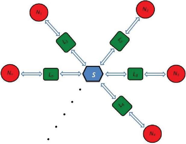
Figure 1 Star configuration system.

3 ${\mathit{\text{L}}}_{\mathit{\text{z}}}$-transform

Consider a Markov process $E(t)$ where each component occupies discrete states and time progresses continuously. This process is characterized by the set of possible states ${\overline{e}}_{i,j}=(e_{i,j}^1,\mathrm{\dots },e_{i,j}^v,\mathrm{\dots },e_{i,j}^V)$, where $e_{i,j}^V$ represents the performance level associated with the distinct performance variable $V$ of component i in any state $j$ $(j=1,\mathrm{\dots },W_i)$, and $W_i$ denotes the total number of possible states, the process is further defined by the transition intensity matrix $X=[x_{ij}(t)]$ and the initial state probability distribution $p_0=[p_{i1},\mathrm{\dots },p_{i{W}_i}]$, where $p_{i1}=\mathrm{Prob}\{E(0)=e_{i,1}^v\}$ and $p_{i{W}_i}=\mathrm{Prob}\{E(0)=e_{i,W_i}^v\}$, for component i in state j. Therefore, the discrete-state, continuous-time Markov process can be defined by the triplet: $E(t)=\{{\overline{e}}_{i,j},X,p_0\}$.

Definition: The $L_z$-transform of a DSCT Markov process $E(t)=\{{\overline{e}}_{i,j},X,p_0\}$ is represented by a function $f(z,t,p_0)$ and expressed as

$$L_z(E(t))=f(z,t,p_0)=\sum _{j=1}^{W_i}{p}_{ij}(t)z^{(e_{i,j}^1,\mathrm{\dots },e_{i,j}^v,\mathrm{\dots },e_{i,j}^V)}.$$

(1)

where, $p_{ij}(t)$ represents the time-dependent probability distribution for the system, indicating the probability of component i being in the state j at time $t\ge 0$. The initial state probabilities are represented by $p_0$, and the expression can be further extended to include the complex variable z.

$L_z$-transform caries with the following properties:

Property 1: If a constant value ‘$a$’ is multiplied by the DSCT Markov process, then it will be multiplied by the corresponding performance level in each state $i$ as

$$L_z(aE(t))=\sum _{j=1}^{W_i}{p}_{ij}(t)z^{a(e_{i,j}^1,\mathrm{\dots },e_{i,j}^v,\mathrm{\dots },e_{i,j}^V)}.$$

Property 2: $L_z$-transform of two DSCT Markov processes $R(t)$ and $S(t)$ from a single-valued function $f(R(t),S(t))$ can be calculated by using Ushakov’s UGF operator ${\mathrm{\Omega }}_f$ to $R(t)$ and $S(t)$ for $t\ge 0$ as

$$L_z\{f[R(t),S(t)]\}={\mathrm{\Omega }}_f(L_z\{R(t)\},L_z\{S(t)\}).$$

(2)

4 Algorithm to Determine the Reliability Measures of An MPMS Weighted Star Configuration System

Consider a system with multiple performance levels and states, organized as a weighted star configuration. In this structure, each component has time-dependent state probabilities, reflecting the evolution of its state over time. The system is designed to be repairable, enabling components to be inspected and maintained to restore their performance. The deterioration of each component is modelled by a Markov process, and repairs are carried out at different intensities depending on the severity of the failure. Minor issues are addressed through preventive maintenance, while more significant failures, such as major failures, require corrective maintenance. In case of complete or major failures, the component is entirely replaced by a new one. Each component in the system operates at multiple performance levels, represented by $\overline{E_i}=(E_i^1,\mathrm{\dots }{E}_i^v,\mathrm{\dots },E_i^V)$ for $1\le v\le V$. For each multi-performance component $E_i^v$ in state $j$, there is a corresponding performance level $e_{i,j}^v$ and the vector ${\overline{e}}_{i,j}$ denotes the performance levels of component $i$ in state $j$, expressed as ${\overline{e}}_{i,j}=(e_{i,j}^1,\mathrm{\dots },e_{i,j}^v,\mathrm{\dots },e_{i,j}^V)$. The multi-performance components in the system exhibit different performance levels ranging from $1,\mathrm{\dots },\mathit{\text{W}}$, where W indicates perfect operation and 1 represents complete failure. The intermediate values between 1 and $W$ correspond to varying degrees of operational effectiveness, reflecting the component’s performance in different states, as shown in Figure 1. Here, each component’s state deteriorates according to a Markov process and follows the (M|M|1):($\mathrm{\infty }$|FCFS) model for repairs or replacement. The state transitions are illustrated in Figure 2.

4.1 Preventive Maintenance

A component can encounter various types of failures, classified as minor, semi-minor, semi-major, or major, each with unique causes and consequences. Minor failures lead to minimal impact on the system’s overall functionality. They may slightly reduce performance or cause minor degradation but are typically easy to resolve. Semi-minor failures represent a greater level of disruption than minor ones, often resulting from moderate interruptions or multiple minor issues occurring together. These failures are typically induced by major disruptions, extensive operational stress, or an accumulation of moderate problems. In terms of preventive maintenance, a component in perfect condition, represented as state $W$, is inspected periodically. Upon inspection, if the component experiences a minor failure, it degrades to state $W-1$. In this case, the system remains operational without requiring immediate maintenance, as the component is effectively restored to between “as good as new” and “as bad as old” condition. However, following a subsequent inspection at state $W-1$, if the component further deteriorates to state $W-2$, preventive maintenance is scheduled. After repair, the component returns to state $W-1$. Following the next inspection at $W-1$, if the component degrades to either state $W-2$ or $W-3$ due to minor or semi-minor failure, preventive maintenance is performed, and the component is restored to its immediate previous state. Specifically, if it falls to state $W-2$, it is restored to $W-1$, and if it falls to state $W-3$, it is restored to state $W-2$. This preventive maintenance cycle continues until the component reaches state 1, representing complete failure.

4.2 Corrective Maintenance

If a component undergoes semi-major or major failure, the nature and impact of the failure differ significantly. A semi-major failure results in severe disruption, causing a direct decline from state $W-1$ or $W-2$ to state 1, which leads to substantial performance loss or system inefficiency. Such failures are typically driven by significant operational strain, major system disruptions, or a combination of multiple moderate-level issues that severely impair the component’s functionality. In contrast, a major failure involves an abrupt and catastrophic transition directly from state $W$ to state 1, signifying total breakdown where the component becomes entirely non-operational and requires replacement instead of repair. When a component reaches state 1 after experiencing either semi-major or major failure, it enters a queueing system for corrective maintenance. The queue operates under an (M|M|1):($\mathrm{\infty }$|FCFS) model, where failures are governed by the Markovian process, and a single technician handles both inspection and corrective maintenance. There is no limit on how many failed components can wait for service, and repairs are performed on a first-come, first-served basis. The technician inspects each failed component to determine whether it can be repaired or must be replaced. If repair is deemed feasible, the repair process follows an Erlang distribution. It is important to recognize that even after repair, the condition of MPMS components does not return to the perfect state $W$. Instead, they occupy a condition between “as good as new” and “as bad as old”. Specifically, when a component degrades to state 1 due to semi-major failure, it is restored to state $W-1$ following inspection and repair rather than being returned to state $W$. The handling of major failure follows a similar queue-based process under the same (M|M|1):($\mathrm{\infty }$|FCFS) model. Major failures often result from catastrophic operational stress or critical system faults leading to total component collapse. Following inspection, if the technician confirms that the failure is beyond repair, the component is scheduled for replacement. The replacement process also follows a first-come, first-served order but adheres to a Weibull distribution model. After replacement, the component is restored to an optimal condition, equivalent to state W or “as good as new.” For instance, when a major failure, represented by ${\lambda }_{4,1}$, occurs, the component transitions from state 1 back to state $W$, achieving full functionality. These sequences of events are illustrated in Figure 2.

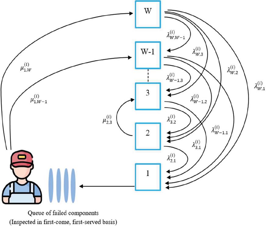
Figure 2 State transition of an MPMS component with minor, semi-minor, semi-major and major failures along with repair and replacement.

Enumerate the set of states corresponding to various performance variables is denoted as ${\overline{e}}_{i,j}=(e_{i,j}^1,\mathrm{\dots },e_{i,j}^v,\mathrm{\dots },e_{i,j}^V)$, where, $e_{i,j}^V$ represents the performance level of a specific performance variable V for component i in state j. The probability distribution $p_0$ is used to describe the initial state probabilities of the MPMS component. With this framework in place, the differential equations governing the probabilities of the transient states can be formulated and expressed as

${\displaystyle \frac{d{p}_{i{W}_i}(t)}{dt}}$	$={\displaystyle \sum _{e=1}^{W_{i-1}}}{\mu }_{e{W}_i}^{(i)}\cdot p_{ie}(t)-p_{iN}(t){\displaystyle \sum _{e=1}^{W_{i-1}}}{\lambda }_{e{W}_i}^{(i)}$	(3)
${\displaystyle \frac{d{p}_{ij}(t)}{dt}}$	$={\displaystyle \sum _{e=j+1}^{W_i}}{\lambda }_{ej}^{(i)}\cdot p_{ie}(t)+{\displaystyle \sum _{e=1}^{j-1}}{\mu }_{ej}^{(i)}\cdot p_{ie}(t)$
	$\mathrm{\hspace{1em}}-p_{ij}(t)\left({\displaystyle \sum _{e=1}^{j-1}}{\lambda }_{je}^{(i)}+{\displaystyle \sum _{e=1}^{W_i}}{\mu }_{je}^{(i)}\right)$	(4)
${\displaystyle \frac{d{p}_{i1}(t)}{dt}}$	$={\displaystyle \sum _{e=2}^{W_i}}{\lambda }_{e1}^{(i)}\cdot p_{ie}(t)-p_{i1}(t){\displaystyle \sum _{e=2}^{W_i}}{\mu }_{ie}^{(i)}$	(5)

The state probability $p_{ij}(t)$ is determined by solving the set of differential equations (3)–(5), utilizing the initial state probability distribution $p_0$. After inspection, if a component in state 1 is found to have undergone a minor, semi-minor, or semi-major failure, the state probability $p_{1,W-1}$ is substituted with the corresponding probability derived from the Erlang distribution, as undermentioned

$$f(t;{\mu }_{1,W-1},{\lambda }_{W-1,1})=\frac{\lambda _{W-1,1}{}^{{\mu }_{1,W-1}}{t}^{{\mu }_{1,W-1}-1}{e}^{-{\lambda }_{W-1,1}t}}{({\mu }_{1,W-1}-1)!}.$$

(6)

where, ${\lambda }_{W-1,1}$ and ${\mu }_{1,W-1}$ denote the semi-major failure rate and the repair rate, respectively, at time $t$. If a major failure is observed during inspection, the probability $p_{1,W}$ is subsequently substituted with the probability computed using the Weibull distribution, as outlined below

$$f(t;{\mu }_{1,W},{\lambda }_{W,1})=\frac{{\lambda }_{W,1}}{{\mu }_{1,W}}{\left(\frac{t}{{\mu }_{1,W}}\right)}^{{\lambda }_{W,1}-1}{e}^{-{\left(\frac{t}{{\mu }_{1,W}}\right)}^{{\lambda }_{W,1}}}.$$

(7)

where, ${\lambda }_{W,1}$ and ${\mu }_{1,W}$ denote the rates of major failure and major repair, respectively. By applying Equations (3) through (7) in conjunction with the multi-state, multi-performance variables ${\overline{e}}_{i,j}=(e_{i,j}^1,\mathrm{\dots },e_{i,j}^v,\mathrm{\dots },e_{i,j}^V)$, the $L_z$-transform for the first component of the system within the framework of the weighted star configuration can be determined as

$$L_z(X_i(t))=f(z,t,p_0)=\sum _{j=1}^{W_i}{p}_{ij}(t)z^{(e_{i,j}^1,\mathrm{\dots },e_{i,j}^v,\mathrm{\dots },e_{i,j}^V)}.$$

(8)

where, $p_{ij}(t)$ denotes the time-dependent probability distribution of the system, capturing the different performance levels and states of its components. The set ${\overline{e}}_{i,j}=(e_{i,j}^1,\mathrm{\dots },e_{i,j}^v,\mathrm{\dots },e_{i,j}^V)$ specifies the performance level of component $i$ in state $j$ at time $t\ge 0$ and $V$ represents the unique performance variables linked to the component. Similarly, the $L_z$-transform for each MPMS component within the system can be calculated individually. There are $k_j$ different demand levels that can be denoted by the set $w_j=[w_{j,1},\mathrm{\dots },w_{j,k_j}]$ corresponding to the node j. Let $e_{i,j}^V$ and $W_j$ denote the random performance variables and demand of the $j^{th}$ generator and node belonging to the set ${\overline{e}}_{i,j}$ and $w_j$, respectively. Additionally, the transmission capacity of the $j^{th}$ transmission line is treated as a random variable, represented by $L_j$ for $j=1,\mathrm{\dots },n$. The set $L_j=[l_{j,1},\mathrm{\dots },l_{j,l_j}]$, denotes all possible random levels of transmission capacity for $L_j$, where $l_{j,l_j}$ indicates the total number of capacity levels.The random demand $W_j$ of the node j assumes values from the set $w_j=[w_{j,1},\mathrm{\dots },w_{j,k_j}]$, then the $L_z$-transform of $W_j$ is expressed as follows

$$L_z(W_j(t))=f(z,t,p_0)=\sum _{j=1}^{k_j}{\gamma }_{ij}(t)z^{(w_{j,1},\mathrm{\dots },w_{j,k_j})}.$$

(9)

In addition, if the random transmission line capacity $L_j$ for the $j^{th}$ transmission line, where $j=1,\mathrm{\dots },n$, is drawn from the set $L_j=[l_{j,1},\mathrm{\dots },l_{j,l_j}]$, then the $L_z$-transform of $L_j$ is defined as

$$L_z(L_j(t))=f(z,t,p_0)=\sum _{j=1}^{l_j}{\delta }_{ij}(t)z^{(l_{j,1},\mathrm{\dots },l_{j,l_j})}.$$

(10)

For any combination of performance levels and demand levels at node j, the surplus performance $M_j$ and performance deficiency $U_j$ exhibit statistical dependence. Specifically, when $M_j>0$, it follows that $U_j=0$, and vice versa. The probability density functions for both $M_j$ and $U_j$ are derived using the$L_z$-transform, which encapsulates both variables. Using the $L_z$-transform $L_z(X_i(t))$ and $L_z(W_j(t))$, the combined $L_z$-transform $(L_z({\wedge }_j(t)))$ can be determined through the application of the composition operator $\otimes$ as

$L_z({\wedge }_j(t))$	$=\otimes (L_z(X_i(t)),L_z(W_j(t)))$
	$={\displaystyle \sum _{j=1}^{W_i}}{p}_{ij}(t)z^{(e_{i,j}^1,\mathrm{\dots },e_{i,j}^v,\mathrm{\dots },e_{i,j}^V)}\otimes {\displaystyle \sum _{j=1}^{k_j}}{\gamma }_{ij}(t)z^{(w_{j,1},\mathrm{\dots },w_{j,k_j})}$
	$={\displaystyle \sum _{j=1}^{W_i}}{\displaystyle \sum _{j=1}^{k_j}}{p}_{ij}(t)\cdot {\gamma }_{ij}(t)\cdot z^{max(0,e_{i,j}^V-w_{j,k_j}),max(0,w_{j,k_j}-e_{i,j}^V)}$	(11)

where, $\max (0,e_{i,j}^V-w_{j,k_j})$ and $\max (0,w_{j,k_j}-e_{i,j}^V)$ are the surplus and deficiency performance of the $j^{th}$ node, denoted as $m_{j,d}$ and $u_{j,d}$, respectively. The system operates effectively for certain predefined weight values that do not require performance sharing from the central node. Therefore, retain only the values that do not meet the predefined weight thresholds $K_1$ and $K_2$, so that they can share the performance to meet the required threshold. Terms that are equal to or exceed these predefined values, which do not necessitate performance sharing, should be excluded from the calculation. Consequently, the $L_z$-transform $(L_z({\wedge }_j(t)))$ is modified by applying the operator $\odot$ as follows

$\otimes ({\wedge }_j(t))$	$=\odot (L_z(X_i(t)),L_z(W_j(t)))=L_z({\vee }_j(t))$
	$={\displaystyle \sum _{j=1}^{W_i}}{\displaystyle \sum _{j=1}^{k_j}}{p}_{ij}(t)\cdot {\gamma }_{ij}(t)$
	$\mathrm{\hspace{1em}}\cdot z^{(max(0,e_{i,j}^V-w_{j,k_j}))<K_1,(max(0,w_{j,k_j}-e_{i,j}^V))<K_2}$	(12)

At node $j^{th}$, if $m_{j,d}>0$, the surplus performance $m_{j,d}$ can be delivered to the central node. Conversely, when the performance is deficient, $u_{j,d}$ must be compensated by drawing resources from the central node via the transmission line $L_j$. The capacity of performance exchange between node j and the central node is constrained by the bandwidth of $L_j$. Consequently, the actual amount of performance transferred is governed by either $\max (L_j,M_j)$ or $\rho (L_j,U_j)$. Let $D_j$ represent the real performance exchanged between node j and the central node. Then the$L_z$-transform for $D_j$ is obtained using the composition operator $\ominus$ as

$L_z(D_j(t))$	$=\ominus (L_z\left({\vee }_j(t)\right),L_z(L_j(t)))$
	$={\displaystyle \sum _{j=1}^{W_i}}{\displaystyle \sum _{j=1}^{k_j}}{p}_{ij}(t)\cdot {\gamma }_{ij}(t)\cdot z^{m_{j,d},u_{j,d}}\ominus {\displaystyle \sum _{j=1}^{l_j}}{\delta }_{ij}(t)z^{(l_{j,1},\mathrm{\dots },l_{j,l_j})}$
	$={\displaystyle \sum _{j=1}^{W_i}}{\displaystyle \sum _{j=1}^{k_j}}{\displaystyle \sum _{j=1}^{l_j}}{p}_{ij}(t)\cdot {\gamma }_{ij}(t)\cdot {\delta }_{ij}(t)\cdot z^{max(m_{j,d},l_{j,d}),max(u_{j,d},l_{j,d})}$	(13)

Once the $L_z$-transform for the entire weighted star configuration system is obtained, the dynamic reliability measures can be computed as described in the following sections.

4.3 Reliability

The reliability of an MPMS weighted star configuration system can be obtained by employing $L_z$-transform for the system’s required minimum threshold performance as

$R(t)={\displaystyle \sum _{j=1}^W}{p}_{ij}(t)\cdot {\gamma }_{ij}(t)\cdot {\delta }_{ij}(t)\cdot \beta [max(m_{j,d},l_{j,d}),max(u_{j,d},l_{j,d})]$

where,

$$\beta (x,y)=\{\begin{array}{cc}1,\hfill & x,y\ge 0\hfill \\ 0,\hfill & x,y<0\hfill \end{array}$$

(14)

4.4 Availability

The MPMS system’s availability can be determined as follows

$A(t)={\displaystyle \sum _{j=1}^W}{p}_{ij}(t)\cdot {\gamma }_{ij}(t)\cdot {\delta }_{ij}(t)\cdot \beta [max(m_{j,d},l_{j,d}),max(u_{j,d},l_{j,d})]$

(15)

While the formulas for system reliability and availability may seem similar at first glance, they are fundamentally different due to the unique treatment of failure rates in each concept. Reliability focuses on the ability of a system to function continuously without failure over a defined time span, without explicitly incorporating failure rates into its calculation. In contrast, availability considers failure rates, reflecting the likelihood that a system is operational and ready for use at any moment in time.

4.5 Mean Expected Performance

The mean expected performance of the entire MPMS system at time $t\ge 0$ is calculated as

$$M(t)=\sum _{\begin{array}{c}j=1\\ e_{i,j}^v>0\end{array}}^{W_i}{p}_{ij}(t)\cdot [max(m_{j,d},l_{j,d}),max(u_{j,d},l_{j,d})].$$

(16)

4.6 Sensitivity

The MPMS system’s instantaneous sensitivity with respect to repair rate $(S_{\mu }(t))$ and failure rate $(S_{\lambda }(t))$ can be evaluated, respectively, as

$S_{\mu }(t)$	$={\displaystyle \frac{\partial A(t)}{\partial \mu }}={\displaystyle \frac{\lambda }{{(\lambda +\mu )}^2}}(1-e^{-(\lambda +\mu )t})-{\displaystyle \frac{t\mu }{\lambda +\mu }}{e}^{-(\lambda +\mu )t}$	(17)
$S_{\lambda }(t)$	$={\displaystyle \frac{\partial A(t)}{\partial \lambda }}=-{\displaystyle \frac{\mu }{{(\lambda +\mu )}^2}}(1-e^{-(\lambda +\mu )t})+{\displaystyle \frac{t\lambda }{\lambda +\mu }}{e}^{-(\lambda +\mu )t}$	(18)

4.7 Cost Analysis

The expected costs or revenues $C(t)$ for the system under consideration over the interval $[0,t]$ are determined using Equation (19). In this context, $S_1$ represents the service facility, whereas $S_2$ indicates the service cost per unit of time within the same period $[0,t]$. This method fundamentally evaluates the service facility’s profitability by assessing the balance between the income produced and the operational costs accrued over the given duration and expressed as

$$C(t)=S_1{\int }_0^{t}A(t)\mathit{d}t-S_{2}t.$$

(19)

Table 1 Transition rates and performance variables of outer ring gear of SSG system

		Transition Rates of
Outer		Outer Ring Gear				Performance Level
Ring Gears	States	S${}_1$	S${}_2$	S${}_3$	S${}_4$	$e_{ij}$
	S${}_{\mathrm{1}}$	0.00	0.00	3.42	4.97	0,0
Ring	S${}_{\mathrm{2}}$	0.98	0.00	4.11	0.00	3,6
Gear 1	S${}_{\mathrm{3}}$	1.32	5.61	0.00	0.00	4,8
	S${}_{\mathrm{4}}$	2.32	2.77	1.49	0.00	5,9
	S${}_{\mathrm{1}}$	0.00	0.00	4.68	4.99	0,0
Ring	S${}_{\mathrm{2}}$	3.78	0.00	3.54	0.00	2,5
Gear 2	S${}_{\mathrm{3}}$	2.19	2.34	0.00	0.00	4,6
	S${}_{\mathrm{4}}$	0.65	1.03	2.22	0.00	6,6
	S${}_{\mathrm{1}}$	0.00	0.00	5.36	7.79	0,0
Ring	S${}_{\mathrm{2}}$	1.46	0.00	3.55	0.00	4,9
Gear 3	S${}_{\mathrm{3}}$	1.05	1.99	0.00	0.00	6,10
	S${}_{\mathrm{4}}$	2.75	1.09	2.71	0.00	7,12

5 Numerical Example: Star-shaped Gear System

Consider a star-shaped gear (SSG) system to examine and demonstrate the reliability measures of a weighted star configuration system. An SSG system consists of a central gear, known as the sun gear, surrounded by multiple smaller gears, called radial gears and a fixed outer ring gear, arranged radially and engaging with the central gear’s teeth. When the central gear rotates, it transmits speed and torque i.e., rotational force to each radial’s gear, which is evenly spaced and meshed between the central and outer ring gear, causing it to rotate in the opposite direction. The fixed outer ring provides additional stability and engages with the radial gears to control torque distribution. This configuration efficiently balances load and provides compact high-torque output. In the considered system, three fixed outer ring gears are connected to three radial gears, forming a star-shaped gear system with the central gear at the center. Each outer ring gear is modelled as an MPMS component and has four possible states, denoted as $S_i$, for $i=1,\mathrm{\dots },4$. State $S_4$ represents optimal functionality, while state $S_1$ indicates complete failure. Intermediate states $S_2$ and $S_3$ represent varying degrees of partial malfunction. Failures of the outer ring gears can occur at minor, semi-major and major levels, and each failure type can be managed through repair or replacement procedures, as detailed in Section 4. Further, each radial gear connected to the outer ring gears has two possible states: $S_1$, which denotes complete failure and $S_2$, representing the perfect state. In the event of a complete failure, the radial gear can be repaired. The central gear, connected to the radial gears, has three possible states: $S_1$ (complete failure), $S_3$ (fully functional) and $S_2$ (intermediate state). The central gear can experience minor, semi-major or major failures and can be repaired or replaced according to the procedures outlined in Section 4. The transition rates of the outer ring gears, radial gears and central gears are listed in Tables 1, 2 and 3, respectively, providing the probabilities for state transitions and performance variations between the different components of the system.

Table 2 Transition rates and performance variables of radial gear of SSG system

		Transition Rates of
		Outer Ring Gear	Demand
Radial Gear	States	S${}_1$	S${}_2$	$e_{ij}$
Radial	S${}_{\mathrm{1}}$	0.0	0.5	2,3
Gear 1	S${}_{\mathrm{2}}$	0.9	0.0	3,4
Radial	S${}_{\mathrm{1}}$	0.0	1.5	1,4
Gear 2	S${}_{\mathrm{2}}$	0.8	0.0	2,6
Radial	S${}_{\mathrm{1}}$	0.0	1.9	4,6
Gear 3	S${}_{\mathrm{2}}$	0.2	0.0	5,10

Table 3 Transition rates and performance variables of central gear of SSG system

		Transition Rates
		of Central Gear			Demand
	States	S${}_{\mathrm{1}}$	S${}_{\mathrm{2}}$	S${}_{\mathrm{3}}$	$e_{ij}$
Central	S${}_{\mathrm{1}}$	0.0	1.8	2.1	1,2
Gear	S${}_{\mathrm{2}}$	0.4	0.0	1.5	3,5
	S${}_{\mathrm{3}}$	0.5	0.2	0.0	6,7

Formulate the governing differential equations that characterize the operation of the MPMS outer ring gear, taking into account minor, semi-major and major failures, along with the processes of repair or replacement, based on Equations (3)–(5) as

${\displaystyle \frac{d{p}_{i1}(t)}{dt}}$	$=({\mu }_{13}^{(i)}+{\mu }_{14}^{(i)})p_{i1}(t)+{\lambda }_{21}^{(i)}{p}_{i2}(t)+{\lambda }_{31}^{(i)}{p}_{i3}(t)+{\lambda }_{41}^{(i)}{p}_{i4}(t)$	(20)
${\displaystyle \frac{d{p}_{i2}(t)}{dt}}$	$=-({\lambda }_{21}^{(i)}+{\mu }_{23}^{(i)})p_{i2}(t)+{\lambda }_{32}^{(i)}{p}_{i3}(t)+{\lambda }_{42}^{(i)}{p}_{i4}(t)$	(21)
${\displaystyle \frac{d{p}_{i3}(t)}{dt}}$	$={\mu }_{13}^{(i)}{p}_{i1}(t)++{\mu }_{23}^{(i)}{p}_{i2}(t)-({\lambda }_{31}^{(i)}+{\lambda }_{32}^{(i)})p_{i3}(t)+{\lambda }_{43}^{(i)}{p}_{i4}(t)$	(22)
${\displaystyle \frac{d{p}_{i4}(t)}{dt}}$	$={\mu }_{14}^{(i)}{p}_{i1}(t)-({\lambda }_{41}^{(i)}+{\lambda }_{42}^{(i)}+{\lambda }_{43}^{(i)})p_{i4}(t)$	(23)

Solving Equations (16)–(19) using the initial conditions $p_{14}(0)=1$ and $p_{13}(0)=p_{12}(0)=p_{11}(0)=0$, we get

$f(t;{\mu }_{13},{\lambda }_{31})$	$={\displaystyle \frac{\lambda _{31}{}^{{\mu }_{13}}{t}^{{\mu }_{13}-1}{e}^{-{\lambda }_{31}t}}{({\mu }_{13}-1)!}}$	(24)
$f(t;{\mu }_{14},{\lambda }_{41})$	$={\displaystyle \frac{{\lambda }_{41}}{{\mu }_{14}}}{\left({\displaystyle \frac{t}{{\mu }_{14}}}\right)}^{{\lambda }_{41}-1}{e}^{-{\left(\frac{t}{{\mu }_{14}}\right)}^{{\lambda }_{41}}}$	(25)

Upon solving Equations (20) through (23), replace the state probabilities $p_{13}$ and $p_{14}$ with the corresponding probability density functions derived from the Erlang and Weibull distributions, with the help of Equations (24) and (25), respectively. Using these substitutions, the state probabilities for the first outer ring gear of the SSG system can be determined as shown in Figure 3.

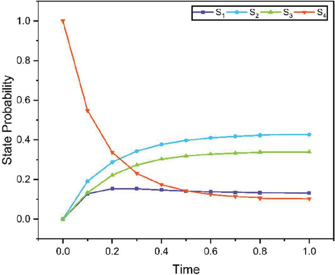
Figure 3 State probabilities of first outer ring gear.

The $L_z$-transform of the first outer ring gear $(X_1)$ with multiple performances can be evaluated using Equation (1) as

$L_z(X_1(t))$	$={\displaystyle \sum _{j=1}^4}{p}_{1j}(t)z^{(e_{1j}^1,e_{1j}^2)}=p_{11}(t)z^{(0,0)}+p_{12}(t)z^{(3,6)}$
	$\mathrm{\hspace{1em}}+p_{13}(t)z^{(4,8)}+p_{14}(t)z^{(5,9)}$

where, $e_{1j}^1$ and $e_{1j}^2$ represent the first and second performance variables for the first outer ring gear in state $j$, respectively. Now, substitute $i=2$ and 3 into Equations (20) through (23) to derive the system of differential equations for the second and third outer ring gears. After solving the system of differential equations so obtained, with the initial conditions $p_{i4}(0)=1$ and $p_{i3}(0)=p_{i2}(0)=p_{i1}(0)=0$, replace the state probabilities $p_{i3}$ and $p_{i4}$, for $i=2$ and 3, using the probability density functions based on the Erlang and Weibull distributions, respectively. After these replacements, the resulting state probabilities for the second and third outer ring gears, are shown in Figures 4 and 5, respectively.

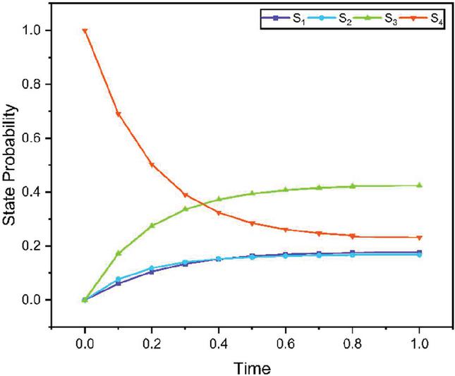
Figure 4 State probabilities of second outer ring gear.

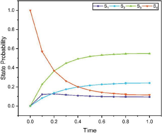
Figure 5 State probabilities of third outer ring gear.

Based on the state probabilities, the $L_z$-transform of the second $(X_2)$ and third $(X_3)$ outer ring gears, each with multiple performances, can be computed using Equation (1) as

$L_z(X_2(t))$	$={\displaystyle \sum _{j=1}^4}{p}_{2j}(t)z^{(e_{2j}^1,e_{2j}^2)}=p_{21}(t)z^{(0,0)}+p_{22}(t)z^{(2,5)}$
	$\mathrm{\hspace{1em}}+p_{23}(t)z^{(4,6)}+p_{24}(t)z^{(6,6)}$
$L_z(X_3(t))$	$={\displaystyle \sum _{j=1}^4}{p}_{3j}(t)z^{(e_{3j}^1,e_{3j}^2)}=p_{31}(t)z^{(0,0)}+p_{32}(t)z^{(4,9)}$
	$\mathrm{\hspace{1em}}+p_{33}(t)z^{(6,10)}+p_{34}(t)z^{(7,12)}$

Similarly, the system of differential equations for the first radial gear can be obtained using Equations (3)–(5) as

$$\begin{array}{cc}\hfill \frac{d{\gamma }_{11}(t)}{dt}& =-0.9{\gamma }_{11}(t)+0.5{\gamma }_{12}(t)\hfill \\ \hfill \frac{d{\gamma }_{12}(t)}{dt}& =0.9{\gamma }_{12}(t)-0.5{\gamma }_{12}(t)\hfill \end{array}\}$$

(26)

Once the Equation (26) is solved under the initial condition ${\gamma }_{12}(0)=1$ and ${\gamma }_{11}(0)=0$, the state probabilities for the first radial gear of the SSG system can be determined as shown in Figure 6.

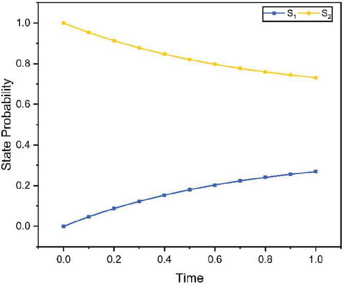
Figure 6 State probabilities of first radial gear.

With the help of state probabilities and the demand values outlined in Table 2. The $L_z$-transform of the first radial gear $(W_1)$ can be computed using Equation (9) as

$L_z(W_1(t))={\displaystyle \sum _{j=1}^2}{\gamma }_{1j}(t)z^{(w_{1,1},w_{1,2})}={\gamma }_{11}(t)z^{(2,3)}+{\gamma }_{12}(t)z^{(3,5)}$

where, $w_{1,1}$ and $w_{1,2}$ represent the required demands and ${\gamma }_{1j}$ is the state probabilities for the first radial gear in the $j^{th}$ state. Likewise, the state probabilities for the other radial gears can be obtained, and using these state probabilities, the $L_z$-transform of the second $(W_2)$ and third $(W_3)$ radial gear can be evaluated as

$L_z(W_2(t))$	$={\displaystyle \sum _{j=1}^2}{\gamma }_{2j}(t)z^{(w_{2,1},w_{2,2})}={\gamma }_{21}(t)z^{(1,4)}+{\gamma }_{22}(t)z^{(2,6)}$
$L_z(W_3(t))$	$={\displaystyle \sum _{j=1}^2}{\gamma }_{3j}(t)z^{(w_{3,1},w_{3,2})}={\gamma }_{31}(t)z^{(4,6)}+{\gamma }_{32}(t)z^{(5,10)}$

Now, the system of differential equation for the transmitter i.e., the central gear, can be obtained as

$$\begin{array}{cc}\hfill \frac{d{\delta }_{11}(t)}{dt}& =-3.9{\delta }_{11}(t)+0.4{\delta }_{12}(t)+0.5{\delta }_{13}(t)\hfill \\ \hfill \frac{d{\delta }_{12}(t)}{dt}& =1.8{\delta }_{11}(t)-1.9{\delta }_{12}(t)+0.2{\delta }_{13}(t)\hfill \\ \hfill \frac{d{\delta }_{13}(t)}{dt}& =2.1{\delta }_{11}(t)+1.5{\delta }_{12}(t)-0.7{\delta }_{13}(t)\hfill \end{array}\}$$

(27)

Solving the Equation (27) under the initial condition ${\delta }_{13}(0)=1$ and ${\delta }_{12}(0)={\delta }_{11}(0)=0$, the state probabilities for the central gear of the SSG system can be computed as illustrated in Figure 7.

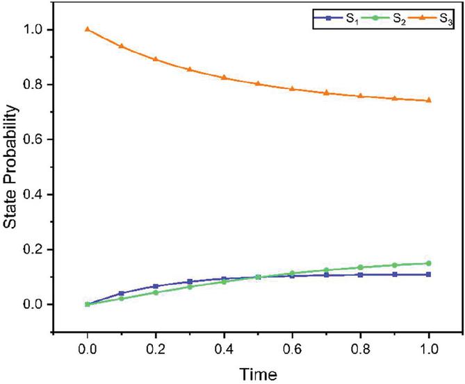
Figure 7 State probabilities of the central gear.

Using the state probabilities and the demand values, the $L_z$-transform for the central gear $(L(t))$ can be calculated using Equation (10) as follows

$L_z(L(t))$	$={\displaystyle \sum _{j=1}^3}{\delta }_{ij}(t)z^{(l_{1,1},l_{1,2})}={\delta }_{11}(t)z^{(1,2)}$
	$\mathrm{\hspace{1em}}+{\delta }_{12}(t)z^{(3,5)}+{\delta }_{13}(t)z^{(6,7)}$

At node j, the surplus performance and performance deficiency are statistically dependent on any combination of performance and demand levels. By utilizing the $L_z$-transform, $L_z(X_1(t))$ and $L_z(W_1(t))$, the combined $L_z$-transform $(L_z({\wedge }_1(t)))$ can be derived using the composition operator $\otimes$, with the help of Equation (11) as

$L_z({\wedge }_1(t))$	$=\otimes (L_z(X_1(t)),L_z(W_1(t)))$
$L_z({\wedge }_1(t))$	$=((p_{11}(t)z^{(0,0)}+p_{12}(t)z^{(3,6)}+p_{13}(t)z^{(4,8)}$
	$\mathrm{\hspace{1em}}+p_{14}(t)z^{(5,9)}),({\gamma }_{11}(t)z^{(2,3)}+{\gamma }_{12}(t)z^{(3,5)}))$	(28)

Likewise, the combined $L_z$-transform $(L_z({\wedge }_2(t)))$ and $(L_z({\wedge }_3(t)))$ can be derived using the composition operator $\otimes$ as

$L_z({\wedge }_2(t))$	$=\otimes (L_z(X_2(t)),L_z(W_2(t)))$
$L_z({\wedge }_2(t))$	$=((p_{21}(t)z^{(0,0)}+p_{22}(t)z^{(2,5)}+p_{23}(t)z^{(4,6)}$
	$\mathrm{\hspace{1em}}+p_{24}(t)z^{(6,6)}),({\gamma }_{21}(t)z^{(1,4)}+{\gamma }_{22}(t)z^{(2,6)}))$	(29)
$L_z({\wedge }_3(t))$	$=((p_{31}(t)z^{(0,0)}+p_{32}(t)z^{(4,9)}+p_{33}(t)z^{(6,10)}$
	$\mathrm{\hspace{1em}}+p_{34}(t)z^{(7,12)}),({\gamma }_{31}(t)z^{(4,6)}+{\gamma }_{32}(t)z^{(5,10)}))$	(30)

Now, remove the values from Equations (28)–(30) that are equal to or exceed the threshold value and do not require performance sharing and retain only those values that fall short of the predefined weight thresholds $K_1$ and $K_2$, as these are the ones that need to share performance to meet the required threshold, as defined in Equation (12). Then the $L_z$-transform $(L_z({\wedge }_j(t)))$ is modified by applying the operator $\odot$ as

$(L_z({\wedge }_j(t)))$	$=\odot (L_z({\wedge }_1(t)),L_z({\wedge }_2(t))L_z({\wedge }_2(t)))=L_z({\vee }_j(t))$
$L_z({\vee }_j(t))$	$=\odot (((p_{11}(t)z^{(0,0)}+p_{12}(t)z^{(3,6)}+p_{13}(t)z^{(4,8)}$
	$\mathrm{\hspace{1em}}+p_{14}(t)z^{(5,9)}),({\gamma }_{11}(t)z^{(2,3)}+{\gamma }_{12}(t)z^{(3,5)})),((p_{21}(t)z^{(0,0)}$
	$\mathrm{\hspace{1em}}+p_{22}(t)z^{(2,5)}+p_{23}(t)z^{(4,6)}+p_{24}(t)z^{(6,6)}),({\gamma }_{21}(t)z^{(1,4)}$
	$\mathrm{\hspace{1em}}+{\gamma }_{22}(t)z^{(2,6)})),((p_{31}(t)z^{(0,0)}+p_{32}(t)z^{(4,9)}$
	$\mathrm{\hspace{1em}}+p_{33}(t)z^{(6,10)}+p_{34}(t)z^{(7,12)}),({\gamma }_{31}(t)z^{(4,6)}$
	$\mathrm{\hspace{1em}}+{\gamma }_{32}(t)z^{(5,10)})))$	(31)

The capacity for performance exchange between the radial gear and the central gear is limited by the bandwidth of $L_j$. Let D represent the actual performance exchanged between the radial gear and the central gear. After filtering out the values that fail to meet the required performance or demand in Equation (31), the $L_z$-transform is combined with the $L_z$-transform of the transmitter. This combination allocates the performance necessary to meet the demand using the composition operator $\ominus$ as defined in the Equation (13). Thus, the $L_z$-transform for D is derived as

$L_z(D(t))$	$=\ominus (L_z({\vee }_j(t)),L_z(L(t)))$
	$=(((p_{11}(t)z^{(0,0)}+p_{12}(t)z^{(3,6)}+p_{13}(t)z^{(4,8)}$
	$\mathrm{\hspace{1em}}+p_{14}(t)z^{(5,9)}),({\gamma }_{11}(t)z^{(2,3)}+{\gamma }_{12}(t)z^{(3,5)})),((p_{21}(t)z^{(0,0)}$
	$\mathrm{\hspace{1em}}+p_{22}(t)z^{(2,5)}+p_{23}(t)z^{(4,6)}+p_{24}(t)z^{(6,6)}),({\gamma }_{21}(t)z^{(1,4)}$
	$\mathrm{\hspace{1em}}+{\gamma }_{22}(t)z^{(2,6)})),((p_{31}(t)z^{(0,0)}+p_{32}(t)z^{(4,9)}+p_{33}(t)z^{(6,10)}$
	$\mathrm{\hspace{1em}}+p_{34}(t)z^{(7,12)}),({\gamma }_{31}(t)z^{(4,6)}+{\gamma }_{32}(t)z^{(5,10)})),({\delta }_{11}(t)z^{(1,2)}$
	$\mathrm{\hspace{1em}}+{\delta }_{12}(t)z^{(3,5)}+{\delta }_{13}(t)z^{(6,7)}))$	(32)

Once the $L_z$-transform of the actual performance exchanged between the radial gear and the central gear is obtained, the reliability measures of the SSG system can be determined.

5.1 Reliability

To assess the reliability of the SSG system, Equations (3) through (5) for the first outer ring gear ($X_1$) at the initial time $t=0$, $p_{i4}=1$ for $i=1,\mathrm{\dots },4$ and $p_{ij}(0)=0$ for $i=1,\mathrm{\dots },4;j=1,\mathrm{\dots },3$ become

${\displaystyle \frac{d{p}_{11}(t)}{dt}}$	$=0.98p_{12}(t)+1.32p_{13}(t)+2.32p_{14}(t)$
${\displaystyle \frac{d{p}_{12}(t)}{dt}}$	$=-0.98p_{12}(t)+5.61p_{13}(t)+2.77p_{14}(t)$
${\displaystyle \frac{d{p}_{13}(t)}{dt}}$	$=-6.93p_{13}(t)+1.49p_{14}(t)$
${\displaystyle \frac{d{p}_{14}(t)}{dt}}$	$=-6.58p_{14}(t)$

Similarly, the system of differential equations governing the behaviour of the remaining gears in the SSG system is constructed by applying indices $i,j=2,3$ and 4 into Equations (20) through (25). The corresponding probabilities for each gear are obtained by solving these differential equations under specified initial conditions. The results of these solutions are graphically represented in Figures 8 to 11.

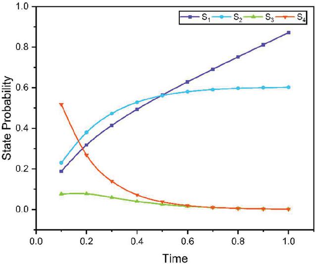
Figure 8 State probabilities of first outer ring gear.

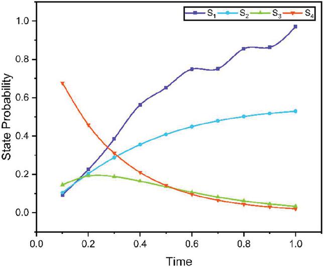
Figure 9 State probabilities of second outer ring gear.

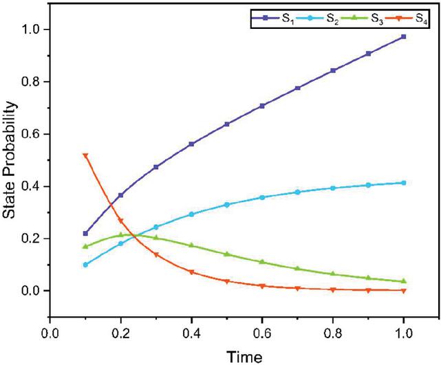
Figure 10 State probabilities of third outer ring gear.

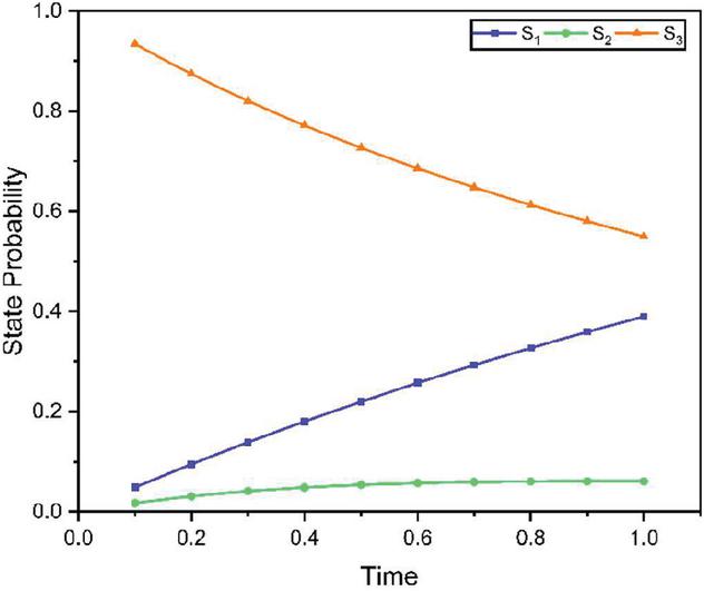
Figure 11 State probabilities of central gear.

After deriving the $L_z$-transform of the actual performance transferred between the radial gear and central gear, incorporating their respective state probabilities, the reliability of the SSG system is computed using Equation (14) by following the procedure detailed in the preceding section. Subsequently, the system’s reliability is determined based on the minimum threshold demand values specific to the SSG system, as illustrated in Figure 12. A three-dimensional plot is presented to depict the reliability trends, highlighting how the system’s reliability responds to varying minimum performance demands over different time intervals.

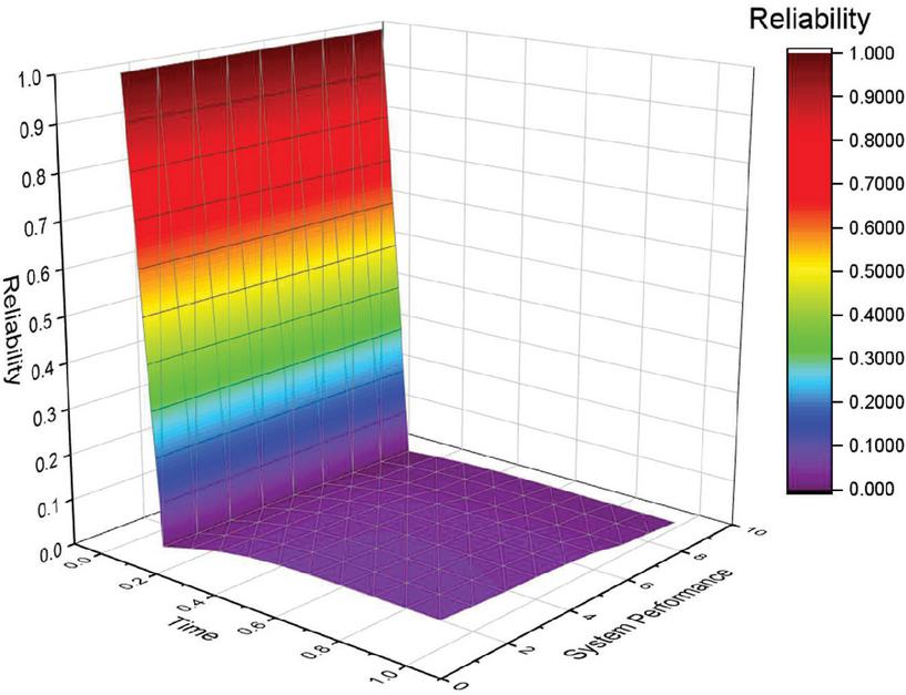
Figure 12 Reliability of SSG system across various performances and time.

5.2 Availability

The computation of the SSG system’s availability follows the method described in Section 4.4 and Equation (15). The resulting availability for the SSG system is displayed in a three-dimensional plot, as depicted in Figure 13. This graphical representation offers a detailed perspective on how availability changes across different time periods, providing insight into the system’s performance over time.

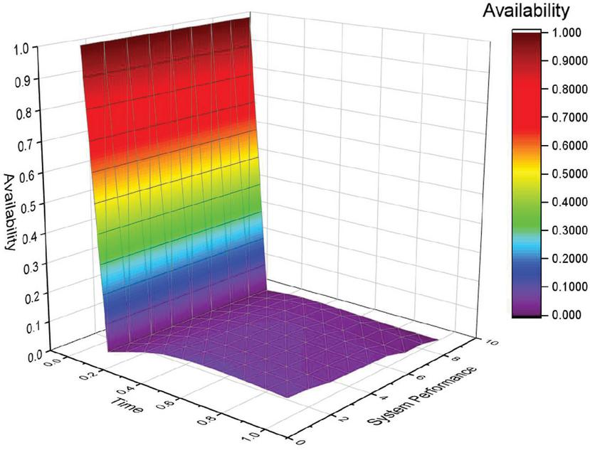
Figure 13 Availability of SSG system across various performances and time.

5.3 Sensitivity Analysis

The sensitivity analysis of the SSG system concerning both the repair rate and failure rate for $t\ge 0$ is carried out using Equations (16) and (17). The outcomes of this analysis are visually represented in Figures 14 and 15, providing insights into the impact of these parameters on system performance.

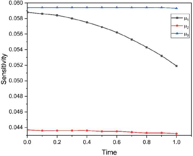
Figure 14 Sensitivity of SSG system with respect to repair rate.

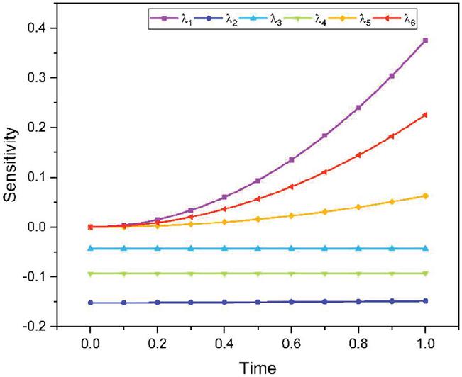
Figure 15 Sensitivity of STP system with respect to failure rate.

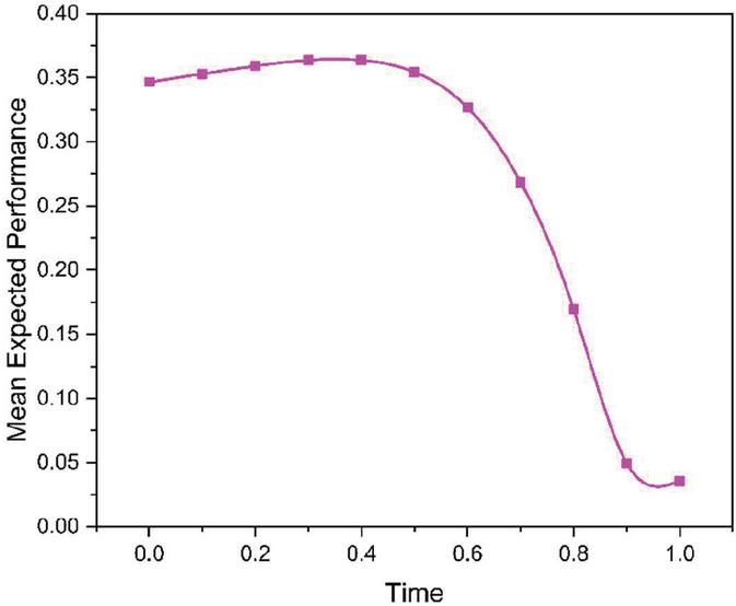
Figure 16 Mean expected performance of SSG system.

5.4 Mean Expected Performance

The instantaneous mean expected performance of the SSG system for time $t\ge 0$ is assessed through Equation (18). The corresponding results are depicted in Figure 16, illustrating how the system’s performance evolves over time.

5.5 Cost Analysis

The expected revenues or costs of the SSG system within the time interval [0, 1] are computed using Equation (19), where the constant revenue cost is set as $G_1=20$, and the service costs vary with values of $G_2=0.05$, 0.04, 0.03, 0.02 and 0.01 per unit. Figure 17 presents the results, offering a visual representation of how the expected revenues or costs change under different service cost conditions.

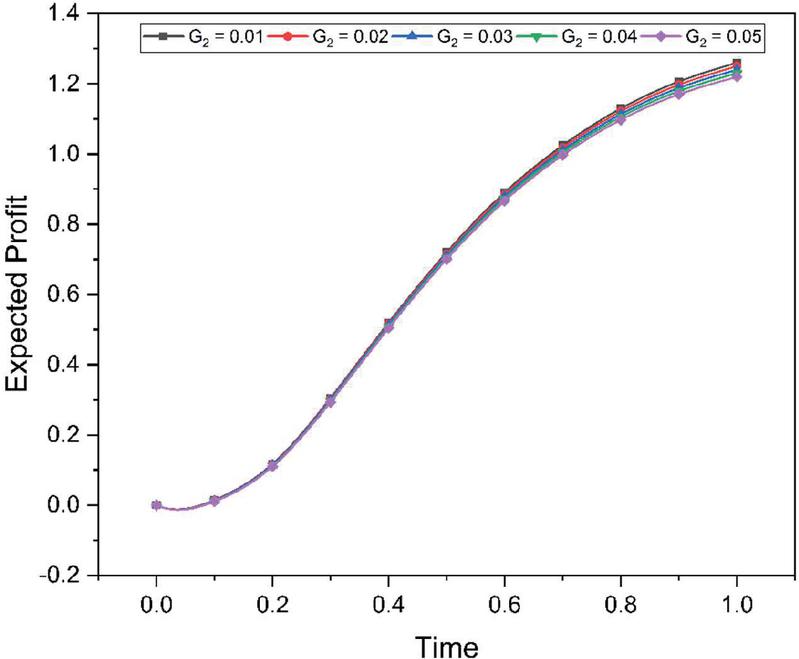
Figure 17 Expected revenue with different service costs for SSG system.

6 Conclusion

The current study explores an MPMS weighted star configuration system designed to handle a range of failure levels, including minor, semi-minor, semi-major and major failures, along with their respective repair and replacement. The star configuration system is structured with a central hub connected to several radial subsystems, each contributing to the overall system performance in a variable manner. The central hub serves as the primary node, coordinating the interaction between the subsystems. In weighted MPMS systems, the state probabilities of individual components fluctuate over time. To address this time-dependent behaviour, a methodology based on the $L_z$-transform is introduced to evaluate the dynamic reliability of the MPMS system, accounting for the time-varying state probabilities of components within a queueing framework. The approach integrates inspection and maintenance strategies for dealing with different types of failure severity. For minor, semi-minor, and semi-major failures, components are repaired following preventive maintenance, whereas major failures require corrective maintenance for their replacement. To validate this approach, a case study of a star-shaped gear system is presented, encompassing various failures. In the event of complete malfunctions, components do not undergo immediate repair or replacement, instead, they enter a queue, awaiting maintenance after inspection. The system operates based on an (M|M|1):($\mathrm{\infty }$|FCFS) queueing model, where repairs follow an Erlang distribution, and replacements follow a Weibull distribution. This queuing structure allows for a more detailed representation of system behaviour, capturing the dynamics of resource allocation and maintenance scheduling. Dynamic reliability, availability, sensitivity, mean expected performance and expected revenue cost are carried out and plotted to illustrate the system’s evolving behaviour. These calculations reveal how the star configuration adapts to varying levels of subsystem performance and the impact of different failure rates on overall system reliability and cost. The ability to model these dynamic interactions between the central hub and the radial subsystems offers deeper insights into system optimization, maintenance policies, and performance enhancement strategies.

For the SSG system, the graphs of reliability and availability in Figures 12 and 13 exhibits a decreasing trend over time, although an apparent increase in availability is observed. This rise reflects the impact of maintenance actions, where the instantaneous uptime improves following the implementation of maintenance procedures. Figure 14 shows that sensitivity remains constant with respect to repair rates, indicating a linear and predictable improvement in availability as the repair rate increases. However, at certain higher repair rates, sensitivity is decreasing because higher repair rates reduce the system’s downtime, making the system’s performance less responsive to further increments in repair efficiency. Conversely, for failure rates, the sensitivity of the SSG system increases over time, as illustrated in Figure 15. This indicates that availability becomes more sensitive to variations in failure frequency, with even slight increments in failure rates causing significant reductions in uptime and making the system more susceptible to disruptions. Figure 16 depicts the decline in the mean expected performance of the SSG system over time, highlighting a reduction in overall efficiency. This decrease may be attributed to factors such as component wear and tear or environmental changes affecting system operation. Additionally, as shown in Figure 17, the expected revenue of the system rises over time with decreasing service cost $G_2$, demonstrating how reduced operational expenses positively influence profitability. The methodology presented in this research is broadly applicable to complex MPMS systems with time-dependent component behaviour, offering a practical framework for evaluating dynamic reliability measures. By accounting for evolving component states and performance levels, this approach provides a robust solution for optimizing reliability in engineering systems under real-world operating conditions.

The proposed model opens avenues for further exploration and refinement in dynamic reliability analysis. While the current study primarily employs the Markov process, future research could explore the integration of Semi-Markov processes. Additionally, investigating alternative queuing models, advanced inspection techniques, and innovative condition-based maintenance strategies presents valuable opportunities to enhance system performance and efficiency.

Competing Interests

The authors declare that they have no conflict of interest.

Data Availability Statement

No specific data has been used in the preparation of the manuscript.

Acknowledgement

The first author gratefully acknowledges the Department of Social Justice and Empowerment (India) for providing the National Fellowship for Scheduled Castes (NSFDC/E-71131) and financial support during this study.

Credit Authorship Contribution Statement

Ayush Singh: Conceptualization, Methodology, Validation, Formal analysis, Investigation, Writing – original draft. S. B. Singh: Conceptualization, Methodology, Validation, Reviewing, Supervision.

References

[1] Bisht, S., and Singh, S. B. (2021). Reliability Evaluation of Repairable Parallel-Series Multi-State System Implementing Interval Valued Universal Generating Function. Journal of Reliability and Statistical Studies, 14(1), 81–120.

[2] Bisht, V., and Singh, S. B. (2021). Reliability estimation of 4$\times$4 SENs using UGF method. Journal of Reliability and Statistical Studies, 14(1), 173–198.

[3] Bisht, V., and Singh, S. B. (2023). $L_z$-transform approach to evaluate reliability indices of multi-state repairable weighted K-out-of-n systems. Quality and Reliability Engineering International, 39(3), 1043–1057.

[4] Bisht, V., and Singh, S. B. (2024). Dynamic reliability measures of weighted k-out-of-n system with heterogeneous components and its application to solar power generating system. Proceedings of the Institution of Mechanical Engineers, Part O: Journal of Risk and Reliability. 1–11. \nolinkurldoi.org/10.1177/1748006X241289014.

[5] Byun, J. E., Noh, H. M., and Song, J. (2017). Reliability growth analysis of k-out-of-N systems using matrix-based system reliability method. Reliability Engineering & System Safety, 165(2017), 410–421.

[6] Chen, Y., and Yang, Q. (2005). Reliability of two-stage weighted-k-out-of-n systems with components in common. IEEE Transactions on Reliability, 54(3), 431–440.

[7] Ding, Y., Zuo, M. J., Lisnianski, A., and Li, W. (2010). A framework for reliability approximation of multi-state weighted k-out-of-n systems. IEEE Transactions on Reliability, 59(2), 297–308.

[8] Eryilmaz, S. (2013). On reliability analysis of a k-out-of-n system with components having random weights. Reliability Engineering & System Safety, 109(2013), 41–44.

[9] Frenkel, I., Lisnianski, A., and Khvatskin, L. (2012). Availability assessment for aging refrigeration system by using $L_z$-transform. Journal of Reliability and Statistical Studies, 5(2), 33–43.

[10] Gao, J., Yao, K., Zhou, J., and Ke, H. (2018). Reliability Analysis of Uncertain Weighted k-out-of-n Systems. IEEE Transactions on Fuzzy Systems, 26(5), 2663–2671.

[11] Guo, Y. (2011). Discussion on the construction of remote multi-point backup in power communication network. Telecommunications for Electric Power System, 32(2), 22–25.

[12] Hu, L., Zhang, Z., Su, P., and Peng, R. (2017). Fuzzy availability assessment for discrete time multi-state system under minor failures and repairs by using fuzzy $L_z$-transform. Eksploatacja i Niezawodność, 19(2), 179–190.

[13] Kumar, S., and Gupta, R. (2022). Working vacation policy for load sharing K-out-of-N: G system. Journal of Reliability and Statistical Studies, 15(2), 583–616.

[14] Larsen, E. M., Ding, Y., Li, Y. F., and Zio, E. (2020). Definitions of generalized multiperformance weighted multi-state K-out-of-n system and its reliability evaluations. Reliability Engineering & System Safety, 199(2020), 105876.

[15] Levitin, G. (2011). Reliability of multi-state systems with common bus performance sharing. IIE Transactions, 43(7), 518–524.

[16] Li, W., and Zuo, M. J. (2008). Reliability evaluation of multi-state weighted k-out-of-n systems. Reliability engineering & system safety, 93(1), 160–167.

[17] Lisnianski, A. 2012. $L_z$-transform for a discrete-state continuous-time Markov process and its applications to multi-state system reliability. In Recent advances in system reliability: Signatures, multi-state systems and statistical inference, ed. A. Lisnianski and I. Frenkel, 79–95.

[18] Lisnianski, A., and Ding, Y. (2009). Redundancy analysis for repairable multi-state system by using combined stochastic processes methods and universal generating function technique. Reliability Engineering & System Safety, 94(11), 1788–1795.

[19] Lisnianski, A., Frenkel, I., and Khvatskin, L. (2021). Modern dynamic reliability analysis for multi-state systems. In Springer Series in Reliability Engineering. Springer.

[20] Negi, S., and Singh, S. B. (2015). Reliability analysis of non-repairable complex system with weighted subsystems connected in series. Applied Mathematics and Computation, 262(2015), 79–89.

[21] Pant, H., Singh, S. B., Pant, S., and Chantola, N. (2020). Availability analysis and inspection optimisation for a competing-risk k-out-of-n: G system. International Journal of Reliability and Safety, 14(2), 168–181.

[22] Singh, A., Bisht, V., and Singh, S. B. (2025). Reliability indices of multi-state repairable m-out-of-r-within-k-out-of-n system using $L_z$-transform method. Communications in Statistics-Theory and Methods, 54(9), 2741–2758.

[23] Singh, V. V., and Poonia, P. K. (2022). Stochastic analysis of k-out-of-n: G type of repairable system in combination of subsystems with controllers and multi-repair approach. Journal of Optimization in Industrial Engineering, 15(1), 121–130.

[24] Su, P., Wang, G., and Duan, F. (2020). Reliability evaluation of a k-out-of-n (G)-subsystem based multi-state system with common bus performance sharing. Reliability Engineering & System Safety, 198(2020), 106884.

[25] Su, P., Wang, G., and Duan, F. (2021). Reliability analysis for k-out-of-(n + 1): G star configuration multi-state systems with performance sharing. Computers & Industrial Engineering, 152(2021), 106991.

[26] Wang, G., Duan, F., and Zhou, Y. (2018). Reliability evaluation of multi-state series systems with performance sharing. Reliability Engineering & System Safety, 173(2018), 58–63.

[27] Wu, J. S., and Chen, R. J. (1994). An algorithm for computing the reliability of weighted-k-out-of-n systems. IEEE Transactions on Reliability, 43(2), 327–328.

[28] Wu, J. S., and Chen, R. J. (1994). Efficient algorithms for k-out-of-n and consecutive weighted-k-out-of-n: F system. IEEE Transactions on Reliability, 43(4), 650–65.

[29] Zhang, T., Xie, M., and Horigome, M. (2006). Availability and reliability of k-out-of-(M+ N): G warm standby systems. Reliability Engineering & System Safety, 91(4), 381–387.

[30] Zhang, Y. (2021). Reliability analysis of randomly weighted k-out-of-n systems with heterogeneous components. Reliability Engineering & System Safety, 205(2021), 107184.

[31] Zhao, X., Wu, C., Wang, S., and Wang, X. (2018). Reliability analysis of multi-state k-out-of-n: G system with common bus performance sharing. Computers & Industrial Engineering, 124(2018), 359–369.

[32] Zhuang, X., Yu, T., Sun, Z., and Song, K. (2022). Reliability and capacity evaluation of multiperformance multi-state weighted $K^{-}$-out-of-n systems. Communications in Statistics Simulation and Computation, 51(10), 6026–6042.

Biographies

Ayush Singh is a Research Scholar in the Department of Mathematics, Statistics and Computer Science at G. B. Pant University of Agriculture and Technology, Pantnagar, Uttarakhand, India. He received his B.Sc. degree from Hemvati Nandan Bahuguna Garhwal University, Srinagar, Uttarakhand in 2019 and his M.Sc. degree from Sri Dev Suman University, Tehri Garhwal, Uttarakhand in 2021. In 2022, he qualified the CSIR-NET exam in Mathematical Sciences. He has published extensively in reputed journals and serves as a reviewer for several esteemed academic publications. His area of research is Reliability Theory.

S. B. Singh is a Professor in the Department of Mathematics, Statistics and Computer Science, at G. B. Pant University of Agriculture and Technology, Pantnagar, India. He has 25 years of experience in teaching and research, working with undergraduate and postgraduate students at engineering colleges and universities. Prof. Singh is a member of the Indian Mathematical Society, Operations Research Society of India, ISST National Society for Prevention of Blindness in India and Indian Science Congress Association. He is a regular reviewer of many books and international/national journals. He has been a member of the organizing committee of many international and national conferences and workshops. He is editor in Chief of the journal “Journal of Reliability and Statistical Studies”. He has authored and co-authored eight books on various courses in Applied and Engineering Mathematics. He has been conferred with four national awards and two times best teacher awards. He has published his research works in national and international journals of repute. His area of research is Reliability Theory.

Journal of Reliability and Statistical Studies, Vol. 18, Issue 1 (2025), 127–164.
doi: 10.13052/jrss0974-8024.1816
© 2025 River Publishers