A Study on Reliability Estimation with Progressively First Failure Censored Data Using xgamma Distribution

Sunita Sharma^1,* and Vinod Kumar²

¹Department of Mathematics, Manipal Institute of Technology, Manipal Academy of Higher Education, Manipal, Karnataka, 576104, India
²Department of Mathematics, Statistics and Computer Science, G.B. Pant University of Agriculture and Technology, Pantnagar, India
E-mail: sunita.sharma@manipal.edu; vinod_kumarbcb@yahoo.com
*Corresponding Author

Received 15 January 2025; Accepted 26 February 2025

Abstract

Progressively first failure censored (PFFC) data plays a pivotal role in reliability theory and life-testing experiments due to its ability to provide comprehensive insights into the reliability of systems and components. This approach facilitates more accurate estimation of reliability metrics and provides valuable insights into the performance and longevity of systems in life-testing experiments. In this article, we explore both classical and Bayesian approaches to estimate the model parameter and reliability characteristics of the xgamma distribution utilizing data from the PFFC dataset. In classical estimation, we analyze maximum likelihood estimators (MLEs) and derive asymptotic confidence intervals (ACIs). Within the Bayesian framework, we evaluate Bayes estimators using both non-informative and gamma informative priors, employing the squared error loss function (SELF) and utilizing Lindley approximation alongside the Metropolis-Hasting (M-H) algorithm. Furthermore, we construct highest probability density (HPD) intervals using the M-H algorithm. To assess the effectiveness of each estimation method, we conduct numerical computations through a simulation study. Lastly, we analyze a real dataset to demonstrate the practical utility of the xgamma distribution within a censoring framework.

Keywords: xgamma distribution, Bayesian estimation, progressively first failure censoring, maximum likelihood estimation, Lindley approximation, M-H algorithm.

1 Introduction

Censoring plays a crucial role in reliability theory and life testing experiments, where the primary focus is on understanding the durability, longevity, or failure times of products or systems. In these contexts, censoring occurs when the exact failure times of some units are not observed or are incomplete due to various reasons such as the study ending before all units fail, loss to follow-up, or technical constraints.

Reliability theory aims to estimate and predict the probability of a product or system operating without failure for a specified period. Censoring allows researchers to include data from units that have not failed up to the end of the study, providing valuable information about the reliability of the product or system beyond the observed failure times. This is especially important in scenarios where failure times may be censored due to units still functioning or the study ending before all units fail. In life testing experiments, censoring is integral to assessing the reliability and durability of products or systems under controlled conditions. Life testing involves subjecting a sample of units to stress or operating conditions until they fail. Censoring allows researchers to record the exact failure times of some units while including data from units that have not failed up to the end of the test. This enables the estimation of reliability metrics such as mean time to failure, failure rate, or survival probability, even when complete failure information is not available for all units. Among the various types of censoring schemes, Type-I and Type-II censoring schemes are widely employed in reliability analysis. In scenarios where the lifespan of goods or objects extends over a considerable duration, the corresponding test duration of an experiment naturally becomes prolonged. Balasooriya (1995) pioneered a failure censoring approach aimed at enhancing cost-effectiveness and efficiency in life testing procedures. This method involves testing k items across n groups, each comprising k items, and conducting simultaneous tests until the initial failure occurs in each group. While this strategy optimizes resources and time, it lacks flexibility for intermittent removal of units during testing. In contrast, Cohen’s (1963) progressive censoring scheme allows for the removal of units at various stages throughout the testing process, offering greater adaptability and control. By leveraging the cost-effectiveness and time-saving benefits inherent in first failure censoring, alongside the capability for intermittent removal offered by progressive censoring, Wu and Kus (2009) amalgamated these approaches. This fusion gave rise to the progressive first failure censoring scheme (PFFCS), a novel life testing strategy designed to enhance efficiency and reliability. The PFFCS stands as a pivotal advancement in reliability theory and lifetime testing, seamlessly blending the advantages of both first failure censoring and progressive censoring techniques. By melding these approaches, PFFCS offers a multifaceted array of benefits. Firstly, its integrated methodology enhances testing efficiency by concurrently conducting tests while permitting intermittent removals, thereby optimizing resource allocation and reducing overall testing duration. This streamlined process translates to tangible cost savings by eliminating unnecessary testing on failed units and conserving resources. Moreover, PFFCS provides unprecedented flexibility by allowing for the removal of units at various stages of testing, empowering experimenters to adapt the procedure to evolving conditions or unforeseen events. This adaptability not only improves the accuracy of reliability estimates but also enhances the overall reliability analysis by ensuring that relevant failure events are observed and recorded. Several authors in the literature have conducted various research studies based on the proposed censoring scheme, demonstrating its efficacy and applicability. For example, Kumar et al., (2023) studied the classical and Bayesian estimation of the model parameter and the reliability characteristics of the Inverse Pareto distribution using Progressively first failure censored data. Ghafouri and Rastogi (2021) considered the estimation of the parameters and reliability analysis of Kumaraswamy distribution under progressively first-failure censoring. Saini et al., (2021) focused on the estimation of stress-strength reliability function for generalized Maxwell failure distribution using progressive first failure censoring. Further, Dube et al., (2016) dealt with the progressively first failure censored Lindley distribution. Abu-Moussa et al., (2023) investigated the statistical inference for the parameters, reliability and hazard functions of the extended Rayleigh distribution using progressively first-failure censored samples. Moreover Bi et al., (2022) derived reliability estimates for the bathtub-shaped distribution based on progressively first failure censoring samples in their study. Fathi et al., (2022) proposed the estimation method for Bayesian and Non-Bayesian reliability and hazard functions for Weibull inverted exponential distribution based on progressively first-failure censoring data. Zhang and Gui (2020) gave the expressions for reliability and failure functions of the Inverted Exponentiated Half-Logistic distribution with progressively first-failure sampling schemes.

The structure of the remaining sections of the article unfolds as follows: Section 2 outlines the methodology employed in this study. Section 3 provides the notations and abbreviations used throughout the study. Section 4 outlines the classical inference procedures for determining the model parameters and assessing their reliability characteristics. Following this, Section 5 delves into Bayesian inference techniques for estimating the model parameters and evaluating its reliability characteristics. A simulation study is detailed in Section 6, providing empirical validation. In Section 7, real datasets are analyzed to demonstrate the applicability of the proposed model and the first-failure censoring scheme. Finally, Section 8 offers concluding remarks summarizing the key findings and implications of the study.

2 Methodology

A first-failure censoring scheme can be defined in the following manner: Let $n$ independent groups, each containing $k$ items, are subjected to a life test. The test will end once a predetermined number of failures, denoted as $s$, is reached. After the occurrence of the first failure at time $Y_1$, $G_1$ surviving groups along with the group experiencing the failure are excluded from the experiment. The process repeats for subsequent failures: at time $Y_2$, $G_2$ surviving groups and the group with the second failure are removed, continuing iteratively. When the experiment experiences its $s^{th}$ failure at time $Y_s$, we remove the remaining live groups, as well as the group where the $s^{th}$ failure happened, from the experiment. The observed failure times, denoted as $Y_1<Y_2<\mathrm{\cdots }<Y_s$, are referred to as progressively first failure censored order statistics due to the progressive censoring plan $\underset{¯}{G}=(G_1,G_2,\mathrm{\dots },G_s)$, where, $G_j$; $j=1,2,\mathrm{\dots },s$ for represents the predetermined number of live groups to be removed at the $j^{th}$ failure, ensuring that $n=s+G_1+G_2+\mathrm{\cdots }+G_s$. Following this, suppose $\underset{¯}{y}=(y_1,y_2,\mathrm{\dots }{y}_s)$ constitute PFFC sample extracted from a continuous population governed by a cdf $F_Y(y)$ and pdf $f_Y(y)$. Consequently, the likelihood function is determined as stated by Wu and Kus (2009) as

$$L(\underset{¯}{y})=C{k}^s\prod _{j=1}^s{f}_Y(y_j){[1-F_Y(y_j)]}^{k(G_j+1)-1},\mathrm{\hspace{0.25em}0}<y_1<y_2\mathrm{\cdots }<y_s<\mathrm{\infty }$$

(1)

where, $C=n(n-G_1-1)(n-G_1-G_2-2)\mathrm{\cdots }(n-G_1-G_2-\mathrm{\cdots }-G_{s-1}-s+1)$.

The xgamma distribution [Sen et al., (2016)] is a vital tool in reliability analysis, offering precise modeling of component lifetimes and failure patterns. Its flexibility accommodates diverse failure mechanisms, enhancing the accuracy of reliability predictions. Additionally, it is adept at capturing both early-life and wear-out phases, crucial for assessing product durability. In the context of censoring procedures, xgamma distribution plays a crucial role in handling incomplete data, a common challenge in survival analysis. By accommodating censored observations, it facilitates the estimation of key parameters such as survival functions and hazard rates, thereby enabling researchers to draw meaningful conclusions from partially observed datasets. This capability is particularly valuable in longitudinal studies, clinical trials, and epidemiological research where censoring is inherent. Furthermore, the xgamma distribution finds widespread application beyond reliability and censoring in fields such as finance, actuarial science, and environmental modeling.

The pdf and cdf of xgamma distribution with random variable $Y$ and parameter $\theta$ are given below:

$$f_Y(y,\theta )=\frac{{\theta }^2}{(1+\theta )}\left(1+\frac{\theta }{2}{y}^2\right)e^{-\theta y},y>0,\theta >0$$

(2)

and the corresponding cumulative distribution function (cdf) is

$$F_Y(y,\theta )=1-\frac{\left(1+\theta +\theta y+\frac{{\theta }^2{y}^2}{2}\right)}{(1+\theta )}{e}^{-\theta y},y>0,\theta >0$$

(3)

The reliability function $R(y)$ and hazard function $h(y)$ are as follows:

$$R(y)=\left(\frac{1+\theta +\theta y+\frac{{(\theta y)}^2}{2}}{1+\theta }\right)e^{-\theta y},y>0,\theta >0$$	(4)
$$h(y)=\frac{{\theta }^2\left(1+\frac{\theta }{2}{y}^2\right)}{(1+\theta +\theta y+\frac{{\theta }^2{y}^2}{2})},y>0,\theta >0$$	(5)

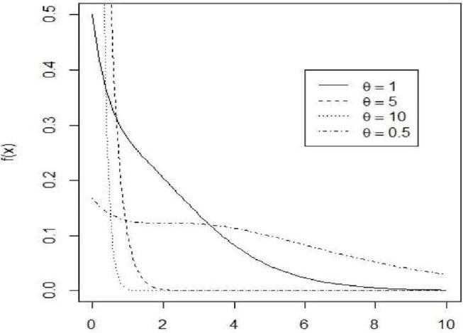
Figure 1 pdf of xgamma for selected values of $\theta$.

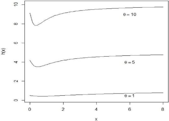
Figure 2 Hazard function of xgamma for selected values of $\theta$.

The survival estimation of xgamma distribution has been discussed by Sen et al., (2018). Yadav et al., (2018) devised maximum likelihood and Bayesian estimation methods for parameter and reliability characterization of the xgamma distribution using hybrid type-II censored samples. Yadav (2023) proposed a Bayesian approach for estimating the parameter and reliability function of the xgamma distribution when dealing with type-I hybrid censored observations. Hence the aim of this paper is to present both classical and Bayesian approaches for inferring the parameters of the xgamma distribution utilizing first-failure censoring schemes. Initially, ML estimates of the parameters and their approximate confidence intervals are obtained. Additionally, employing a symmetric loss function, expressions are derived for the Bayesian estimates of the parameters and reliability characteristics of the model. Due to the complexity of these expressions, which cannot be simplified into closed forms, we employ the Lindley method and the M-H algorithm to compute the Bayesian estimates. Furthermore, we derive HPD credible intervals to provide comprehensive insights into the uncertainty associated with the estimates.

3 Notations and Abbreviations

PFFCS	Progressively first failure censoring scheme
ACI	Asymptotic confidence interval
SELF	Square error loss function
MLE	Maximum likelihood estimate
M-H	Metropolis-Hasting
$\theta$	Parameter of xgamma distribution
$\underset{¯}{y}$	PFFC samples
$L$($\underset{¯}{y}$)	Likelihood function of $\underset{¯}{y}$
$\widehat{R}(\underset{¯}{y})$	MLE of the reliability function of $\underset{¯}{y}$
$\widehat{h}(\underset{¯}{y})$	MLE of the hazard function of $\underset{¯}{y}$
$\pi \left(\theta |\underset{¯}{y}\right)$	Posterior distribution of $\theta$
$R_L^B(\underset{¯}{y})$	Bayes estimate of $R(\underset{¯}{y}$) using Lindley approximation
$h_L^B(\underset{¯}{y})$	Bayes estimate of $h(\underset{¯}{y})$ using Lindley approximation
${\theta }_{MH}^B$	Bayes estimate of $\theta$ using M-H algorithm under SELF
$R_{MH}^B(\underset{¯}{y})$	Bayes estimate of $R(\underset{¯}{y})$ using M-H algorithm under SELF
$h_{MH}^B(\underset{¯}{y})$	Bayes estimate of $h(\underset{¯}{y})$ using M-H algorithm under SELF
CS	Censoring schemes
HPD	Highest posterior density
AL	Average length
CP	Coverage probability
AE	Average estimates
MSE	Mean square error
MCMC	Markov Chain Monte Carlo

4 Classical Estimation

In this section, our primary objective is to estimate the unknown parameter, denoted as $\theta$, associated with xgamma distribution. We derive the MLE for parameter $\theta$ and further explore reliability characteristics such as $R(y)$ and $h(y)$. Furthermore, we develop asymptotic and bootstrap confidence intervals for the parameter $\theta$. Additionally, we establish both asymptotic and bootstrap confidence intervals for the parameter $\theta$. Given a predetermined sampling plan $\underset{¯}{G}=(G_1,G_2,\mathrm{\dots },G_s)$, let $y_1,y_2,\mathrm{\dots }{y}_s$ denote the PFFC sample drawn from the xgamma distribution. Utilizing Equations (1), (2) and (3), we can derive the associated likelihood function as

$L(\underset{¯}{y},\theta )$	$=C{k}^s{\displaystyle \frac{{\theta }^{2s}}{{(1+\theta )}^s}}{\displaystyle \prod _{j=1}^s}\left(1+{\displaystyle \frac{{\theta }^2}{2}}{y}_j^2\right)e^{-\theta y_j}$
	$\mathrm{\hspace{1em}}\times {\left[\left({\displaystyle \frac{1+\theta +\theta y_j+\frac{{(\theta y_j)}^2}{2}}{1+\theta }}\right)e^{-\theta y_j}\right]}^{k(G_j+1)-1}$	(6)

The corresponding log-likelihood function will be

$l(\underset{¯}{y},\theta )$	$=A+2slog\theta -slog(1+\theta )+{\displaystyle \sum _{j=1}^s}\log \left(1+{\displaystyle \frac{{\theta }^2}{2}}{y}_j^2\right)-\theta y_j$
	$\mathrm{\hspace{1em}}+{\displaystyle \sum _{j=1}^s}[k(G_j+1)-1]\log \left({\displaystyle \frac{1+\theta +\theta y_j+\frac{{(\theta y_j)}^2}{2}}{1+\theta }}\right)-\theta y_j$	(7)

where, $A=\log C+s\log k$. Now, the MLE of $\theta$ is given by solution of the following normal equation

${\displaystyle \frac{\partial l(\underset{¯}{y},\theta )}{\partial \theta }}$	$={\displaystyle \frac{2s}{\theta }}-{\displaystyle \frac{s}{(1+\theta )}}+{\displaystyle \sum _{j=1}^s}{\displaystyle \frac{\theta y_j^2}{\left(1+\frac{{\theta }^2}{2}{y}_j^2\right)}}-y_j$
	$\mathrm{\hspace{1em}}+{\displaystyle \sum _{j=1}^s}[k(G_j+1)-1]{\displaystyle \frac{\left[y_j+\theta y_j^2+\frac{{(\theta y_j)}^2}{2}\right]}{\left(\frac{1+\theta +\theta y_j+\frac{{(\theta y_j)}^2}{2}}{1+\theta }\right)}}-y_j=0$	(8)

Obtaining the MLE for $\theta$, denoted as $\widehat{\theta }$, requires solving Equation (4). However, Equation (4) does not offer a closed-form solution, necessitating the use of numerical iterative methods for precise computation of $\widehat{\theta }$. Utilizing the invariance property of MLE, we can then derive estimators for $R(\underset{¯}{y})$ and $h(\underset{¯}{y})$ respectively as follows

$$\widehat{R}\left(\underset{¯}{y}\right)=\left(\frac{1+\widehat{\theta }+\widehat{\theta }y+\frac{{(\widehat{\theta }y)}^2}{2}}{1+\widehat{\theta }}\right)e^{-\widehat{\theta }y}$$

(9)

and

$$\widehat{h}(\underset{¯}{y})=\frac{{\widehat{\theta }}^2\left(1+\frac{\widehat{\theta }}{2}{y}^2\right)}{\left(1+\widehat{\theta }+\widehat{\theta }y+\frac{{\widehat{\theta }}^2{y}^2}{2}\right)}$$

(10)

Under the regular conditions, the MLE $\widehat{\theta }$ is asymptotically normally distributed, i.e., $\widehat{\theta }\sim N(\theta ,I^{-1}(\theta ))$, where $I(\widehat{\theta })$ is observed the Fisher information is given by

$$I(\widehat{\theta })=-E{\left[\frac{{\partial }^{2}l(\underset{¯}{y},\theta )}{\partial {\theta }^2}\right]}_{\theta =\widehat{\theta }}$$

(11)

Here

${\displaystyle \frac{{\partial }^{2}l(\underset{¯}{y},\theta )}{\partial {\theta }^2}}$	$=-{\displaystyle \frac{2s}{{\theta }^2}}+{\displaystyle \frac{s}{{(1+\theta )}^2}}+{\displaystyle \sum _{j=1}^s}{y}_j^2\left[{\displaystyle \frac{1-\frac{{\left(\theta y_j\right)}^2}{2}}{{\left(1+\frac{{\left(\theta y_j\right)}^2}{2}\right)}^2}}\right]$
	$\mathrm{\hspace{1em}}+{\displaystyle \sum _{j=1}^s}[k(G_j+1)-1](y_j^2+\theta y_j^2){\displaystyle \frac{\left(1+\theta +\theta y_j+\frac{{\left(\theta y_j\right)}^2}{2}\right)}{(1+\theta )}}$
	$\mathrm{\hspace{1em}}-{\left[{\displaystyle \frac{y_j+\theta y_j^2+\frac{{\left(\theta y_j\right)}^2}{2}}{(1+\theta )}}\right]}^2$	(12)

If $\widehat{V}ar(\widehat{\theta })=I^{-1}(\widehat{\theta })$ represents the observed variance of $\widehat{\theta }$, then the asymptotic confidence interval for $\widehat{\theta }$ can be derived as follows:

$$\widehat{\theta }\pm z_{\alpha /2}\sqrt{\widehat{V}ar(\widehat{\theta })}$$

Here, $z_{\alpha /2}$ is the upper ${(\alpha /2)}^{th}$ percentile of the standard normal distribution $N(0,1)$. Also, the CP for $\theta$ is given by,

$$C{P}_{\theta }=\left[\frac{\widehat{\theta }-\theta }{\sqrt{\widehat{V}ar(\widehat{\theta })}}\right]\le z_{\alpha /2}$$

5 Bayes Estimation

In this section, we aim to determine the Bayes estimates for the parameter $\theta$ and the reliability characteristics $R(\theta )$ and $h(\theta )$ under the SELF. Assume that the prior belief regarding the unknown parameter $\theta$ follows a gamma distribution with hyperparameters $a$ and $b$. Consequently, the corresponding prior distribution for $\theta$ is given by:

$$h(\theta )=\frac{b^a}{\mathrm{\Gamma }(a)}{\theta }^{a-1}{e}^{-b\theta },\theta >0,a,b>0$$

By incorporating a prior belief in the maximum likelihood function in (4), the posterior distribution of $\theta$ is given by,

$\pi (\theta |\underset{¯}{y})\propto {\displaystyle \frac{\begin{array}{c}\frac{{\theta }^{2s+a-1}}{{(1+\theta )}^s}\exp \left\{-\theta \left(b-{\prod }_{j=1}^s\left(1+\frac{{\theta }^2}{2}{y}_j^2\right)+y_j\right)\right\}\hfill \\ \times \exp \left({\sum }_{j=1}^s[k(G_j+1)-1]\log \left(\frac{1+\theta +\theta y_j+\frac{{\left(\theta y_j\right)}^2}{2}}{1+\theta }\right)\right)\hfill \end{array}}{\begin{array}{c}{\int }_0^{\mathrm{\infty }}\frac{{\theta }^{2s+a-1}}{{(1+\theta )}^s}\exp \left\{-\theta \left(b-{\prod }_{j=1}^s\left(1+\frac{{\theta }^2}{2}{y}_j^2\right)+y_j\right)\right\}\hfill \\ \times \exp \left({\sum }_{j=1}^s[k(G_j+1)-1]\log \left(\frac{1+\theta +\theta y_j+\frac{{(\theta y_j)}^2}{2}}{1+\theta }\right)\right)d\theta \hfill \end{array}}}$

(13)

The posterior distribution given in Equation (13) does not have any closed form solution, so it is quite difficult to obtain the posterior mean analytically. To solve this integration, we propose the following approximation methods: (i) Lindley approximation and (ii) M-H algorithm which are discussed in the next section.

5.1 Lindley Approximation

The Lindley approximation [Lindley (1980)] procedure is used to compute the Bayes estimates of the parameter and the reliability characteristics. Let $u(\theta )$ be any arbitrary function, then its posterior expectation is expressed as,

$$E(u(\theta )/\underset{¯}{y})=\frac{\int u(\theta )v(\theta )e^{l(\theta )}\mathit{d}\theta }{\int v(\theta )e^{l(\theta )}\mathit{d}\theta }$$

where $u(\theta )$ is the function of $\theta$ only, $v(\theta )$: prior density function and $l(\theta )=$ log likelihood function.

Using Lindley’s approximation, $E(u(\theta )/\underset{¯}{y})$ approximately estimated by

$E(u(\theta )/\underset{¯}{y})$	$=[u+0.5{\displaystyle \sum _i}{\displaystyle \sum _j}(u_{ij}+2u_i{\rho }_j){\sigma }_{ij}$
	$\mathrm{\hspace{1em}}+0.5{\displaystyle \sum _i}{\displaystyle \sum _j}{\displaystyle \sum _k}{\displaystyle \sum _l}{L}_{ijk}{\sigma }_{ij}{\sigma }_{kl}{u}_l]+o({\displaystyle \frac{1}{n^2}})$

Here $i,j,k,l=1,2,\mathrm{\dots },n;\theta =({\theta }_1,{\theta }_2,\mathrm{\dots },{\theta }_n);u_i=\frac{\partial u}{\partial {\theta }_i};u_{ij}=\frac{{\partial }^{2}u}{\partial {\theta }_i\partial {\theta }_j};$

$L_{ij}=\frac{{\partial }^{2}l}{\partial {\theta }_i{\theta }_j},{\rho }_i=\frac{\partial \rho }{\partial {\theta }_i}$ where $\rho$ is the logarithm of prior distribution.

In the scenario under consideration, we find that

${\rho }_1$	$={\displaystyle \frac{(a-1)}{\theta }}-b$
$L_{11}$	$={\displaystyle \frac{{\partial }^{2}l}{\partial {\theta }^2}}=-{\displaystyle \frac{2s}{{\theta }^2}}+{\displaystyle \frac{s}{{(1+\theta )}^2}}+{\displaystyle \sum _{j=1}^s}{y}_j^2\left[{\displaystyle \frac{1-\frac{{\left(\theta y_j\right)}^2}{2}}{{\left(1+\frac{{\left(\theta y_j\right)}^2}{2}\right)}^2}}\right]$
	$\mathrm{\hspace{1em}}+{\displaystyle \sum _{j=1}^s}[k(G_j+1)-1](y_j^2+\theta y_j^2){\displaystyle \frac{\left(1+\theta +\theta y_j+\frac{{\left(\theta y_j\right)}^2}{2}\right)}{(1+\theta )}}$
	$\mathrm{\hspace{1em}}-{\left[{\displaystyle \frac{y_j+\theta y_j^2+\frac{{\left(\theta y_j\right)}^2}{2}}{\left(1+\theta \right)}}\right]}^2$
$L_{111}$	$={\displaystyle \frac{4s}{{\theta }^3}}-{\displaystyle \frac{2s}{{(1+\theta )}^3}}+{\displaystyle \sum _{j=1}^s}{y}_j^2\theta y_j^2{\displaystyle \frac{\left[1-2\left(1+\frac{{\left(\theta y_j\right)}^2}{2}\right)\right]}{{\left(1+\frac{{\left(\theta y_j\right)}^2}{2}\right)}^2}}$
	$\mathrm{\hspace{1em}}+{\displaystyle \sum _{j=1}^s}[k(G_j+1)-1]y_j^2\left[{\displaystyle \frac{1+\theta +\theta y_j+\frac{{\left(\theta y_j\right)}^2}{2}}{\left(1+\theta \right)}}\right]$
	$\mathrm{\hspace{1em}}-{\displaystyle \frac{y_j^2}{(1+\theta )}}\left(\theta y_j^2+{\displaystyle \frac{{\left(\theta y_j\right)}^2}{2}}\right)-2\left[{\displaystyle \frac{y_j+\theta y_j^2+\frac{{\left(\theta y_j\right)}^2}{2}}{\left(1+\theta \right)}}\right]$
	$\mathrm{\hspace{1em}}+{\displaystyle \frac{y_j^2(1+\theta )+{(\theta y_j)}^2-2y_j}{2{(1+\theta )}^2}}$

${\sigma }_{ij},i,j=1,2$ are obtained by using $L_{ij},i,j=1,2$.

${\sigma }_{11}$	$={[-L_{11}]}^{-1}=[-{\displaystyle \frac{2s}{{\theta }^2}}+{\displaystyle \frac{s}{{(1+\theta )}^2}}+{\displaystyle \sum _{j=1}^s}{y}_j^2\left[{\displaystyle \frac{1-\frac{{(\theta y_j)}^2}{2}}{{\left(1+\frac{{(\theta y_j)}^2}{2}\right)}^2}}\right]$
	$\mathrm{\hspace{1em}}+{\displaystyle \sum _{j=1}^s}[k(G_j+1)-1](y_j^2+\theta y_j^2){\displaystyle \frac{\left(1+\theta +\theta y_j+\frac{{(\theta y_j)}^2}{2}\right)}{(1+\theta )}}$
	$\mathrm{\hspace{1em}}-{\left[{\displaystyle \frac{y_j+\theta y_j^2+\frac{{(\theta y_j)}^2}{2}}{(1+\theta )}}\right]}^2]{}^{-1}$

First, we consider $u=R(y)$

$u_1$	$={\displaystyle \frac{\partial u}{\partial \theta }}=-y{e}^{-\theta y}\left[{\displaystyle \frac{1+\theta +\theta y+\frac{{(\theta y)}^2}{2}}{(1+\theta )}}\right]+e^{-\theta y}\left[{\displaystyle \frac{y+\theta y^2+\frac{{(\theta y)}^2}{2}}{{(1+\theta )}^2}}\right]$
$u_{11}$	$={\displaystyle \frac{{\partial }^{2}u}{{\partial }^2\theta }}={\displaystyle \frac{-y{e}^{-\theta y}}{(1+\theta )}}\left[{\displaystyle \frac{y+\theta y^2+\frac{{(\theta y)}^2}{2}}{(1+\theta )}}+\left(1+\theta +\theta y+{\displaystyle \frac{{(\theta y)}^2}{2}}\right)\right]$

The Bayes estimate of reliability $R(\underset{¯}{y})$ denoted by $R_L^B$ using the Lindley approximation under SELF is given by

$$R_L^B(\underset{¯}{y})=R(y)+\frac{1}{2}[u_{11}{\sigma }_{11}]+u_1{\rho }_1{\sigma }_{11}+\frac{1}{2}[L_{111}{u}_1{\sigma }_{11}^2]$$

(14)

All the expressions in the above equations are obtained using MLE of the parameters.

In second case, we take $v=h(y)$

$v_1$	$={\displaystyle \frac{\partial v}{\partial \theta }}=\left[{\displaystyle \frac{\begin{array}{c}\frac{{(\theta y)}^2}{2}+2\theta \left(1+\frac{\theta y^2}{2}\right)\left(1+\theta +\theta y+\frac{{(\theta y)}^2}{2}\right)\hfill \\ -{\theta }^2\left(1+\frac{\theta y^2}{2}\right)(1+t+\theta y^2)\hfill \end{array}}{{\left(1+\theta +\theta y+\frac{{(\theta y)}^2}{2}\right)}^2}}\right]$
$v_{11}$	$={\displaystyle \frac{{\partial }^{2}v}{{\partial }^2\theta }}={\displaystyle \frac{1}{{\left(1+\theta +\theta y+\frac{{(\theta y)}^2}{2}\right)}^4}}$
	$\mathrm{\hspace{1em}}\times [\theta (2+\theta y^2)(1+t+\theta y^2)+2(1+\theta y^2)(1+\theta +\theta y+{\displaystyle \frac{{(\theta y)}^2}{2}})$
	$\mathrm{\hspace{1em}}-{(\theta y)}^2\left(1+{\displaystyle \frac{{\theta }^2}{2}}\right)+2\theta \left(1+{\theta }^2\right)\left(1+y+\theta y^2\right)$
	$\mathrm{\hspace{1em}}\times {(1+\theta +\theta y+{\displaystyle \frac{{(\theta y)}^2}{2}})}^2]$
	$\mathrm{\hspace{1em}}-[(1+\theta +\theta y+{\displaystyle \frac{{(\theta y)}^2}{2}})\{\theta (2+\theta y^2\}$
	$\mathrm{\hspace{1em}}-2{\theta }^2(1+{\displaystyle \frac{{\theta }^2}{2}})(1+y+\theta y^2]$

The Bayes estimate of $h(\underset{¯}{y})$ using the Lindley approximation under SELF is given by

$$h_L^B(\underset{¯}{y})=h(y)+\frac{1}{2}\left[v_{11}{\sigma }_{11}\right]+v_1{\rho }_1{\sigma }_{11}+\frac{1}{2}[L_{111}{v}_1{\sigma }_{11}^2]$$

(15)

5.2 M-H Algorithm

The M-H algorithm, a widely utilized MCMC technique, serves to generate a sequence of samples representing the posterior distribution. Gelman et al. (2013) and related references provide comprehensive insights into its application. For an in-depth exploration of the MCMC method and the M-H algorithm, refer to the comprehensive discussions by Metropolis et al. (1953) and Hastings (1970). To generate the random samples from the posterior density of $\theta$ a normal proposal distribution is utilized. The steps of an M-H algorithm are carried out as follows:

Step 1. Start with an initial guess value of $\theta$ say ${\theta }^{(0)}.$

Step 2. Using the M-H algorithm, generate ${\theta }_k^{(h)}$ from $N({\theta }^{(h)}|{\theta }^{(h-1)}).$

Step 3. Generate $u$ from a uniform distribution $U(0,1)$.

Step 4. Compute the value $A({\theta }^{(h)}|{\theta }^{(h-1)})=\min \{\frac{\pi ({\theta }^{(h)}|\underset{¯}{y})N({\theta }^{(h-1)}|{\theta }^{(h)}}{\pi ({\theta }^{(h-1)}|\underset{¯}{y})N({\theta }^{(h)}|{\theta }^{(h-1)}},1\}$

Step 5. If $u\le A,$ set ${\theta }^{(h)}={\theta }_k^{(h)}$ with acceptance rate $A$ otherwise ${\theta }^{(h)}={\theta }^{(h-1)}$.

Step 6. To obtain the parameter sequence of $\theta$, repeat steps 1–5, for $j=1,2,\mathrm{\dots }M,$ say $({\theta }^{(1)},{\theta }^{(2)},{\theta }^{(3)},\mathrm{\dots },{\theta }^{(M)})$.

As a result, we derive the estimate utilizing the $(M-M_0)$ observations, where $M_0$ represents the burn-in period. The approximate Bayes estimate of $g(\theta )$ using M-H algorithm under SELF is expressed as:

$$g_{MH}^B(\theta )=\frac{1}{M-M_0}\sum _{j=M_0+1}^{M}g({\theta }^{(j)})$$

Therefore, the Bayes estimates of the parameter $\theta$ and the reliability characteristics $R(\underset{¯}{y})$ and $h(\underset{¯}{y)}$ under SELF using M-H algorithm, respectively are expressed as

${\theta }_{MH}^B$	$={\displaystyle \frac{1}{M-M_0}}{\displaystyle \sum _{j=M_0+1}^M}{\theta }^{(j)}$
$R_{MH}^B(\underset{¯}{y})$	$={\displaystyle \frac{1}{M-M_0}}{\displaystyle \sum _{j=M_0+1}^M}\left({\displaystyle \frac{1+{\theta }^{(j)}+{\theta }^{(j)}y+\frac{{({\theta }^{(j)}y)}^2}{2}}{1+{\theta }^{(j)}}}\right)e^{-{\theta }^{(j)}y}\mathit{\hspace{1em}}\text{and}$
$h_{MH}^B(\underset{¯}{y})$	$={\displaystyle \frac{1}{M-M_0}}{\displaystyle \sum _{j=M_0+1}^M}{\displaystyle \frac{{({\theta }^{(j)})}^2\left(1+\frac{{\theta }^{(j)}}{2}{y}^2\right)}{\left(1+{\theta }^{(j)}+{\theta }^{(j)}y+\frac{{({\theta }^{(j)})}^2{y}^2}{2}\right)}}$

Next, we calculate the HPD credible interval, as presented below:

The HPD interval of $\theta$ can be obtained using sample generated by M-H algorithm. Let ${\theta }_{(1)}<{\theta }_{(2)}<\mathrm{\cdots }<{\theta }_{(M)}$. Now by using the algorithm proposed by Chen and Shao (1999), the $100(1-\eta )\%$, where, $0<\eta <1$, HPD credible interval of $\theta$ will be $({\theta }_{(j)},{\theta }_{(j+[(1-\eta )M])})$, where $j$ is chosen such that

${\theta }_{(j+[(1-\eta )M])}-{\theta }_{(j)}=\underset{1\le i\le \eta M}{\min }({\theta }_{(i+[(1-\eta )M])}-{\theta }_{(j)}),j=1,2,\mathrm{\dots }M,$

where, $[x]$ is the integer part of $x$.

6 Simulation Study

We employ a Monte Carlo simulation in this section to demonstrate the effectiveness of the estimation strategies proposed in this paper. In this study, PFFC samples are generated for various combinations of $(n,k,s)$ with a predefined censoring plan $\underset{¯}{G}$, alongside distinct values of the model parameter $\theta$. We utilize the algorithm proposed by Balakrishnan and Sandhu (1995) with some modifications to generate these samples. This adaptation enables the PFFC sample $y_1,y_2,\mathrm{\dots }{y}_s$ to be interpreted as a progressively censored sample derived from a population characterized by the cdf $[1-{(1-F(y))}^k]$ (Wu and Kus (2009)). For the simulation, we consider various combinations of $k$, $n$, and $s$. The number of items within each group $k$ ranges from 2 to 4, the number of groups $n$ varies from 20 to 30, and the predetermined number of failures $s$ represents 60$\%$ to 80$\%$ of $n$, all with a prefixed censoring plan $\underset{¯}{G}$. Additionally, we select two distinct representative values for $\theta$ as $\theta =0.5$ and $\theta =1.5$, respectively. For simulation purposes, a value of $\theta =1.5$ has been chosen. For every value of $n$, there are four distinct failure strategies implemented, with three of them being consistent across all scenarios. These three shared failure strategies are outlined below:

Scheme 1: $\{(k,n,s),(G_1=n-s,G_i=0,\forall i=2,3,\mathrm{\dots }s)\}$. In this scenario, at the first instance of failure, $(n-s)$ groups are eliminated from the experiment.

Scheme 2: $\{(k,n,s),(G_i=0,\forall i=1,2,\mathrm{\dots }s-1,G_s=n-s)\}.$ In this scenario, groups are removed at the $s^{th}$ failure, and

Scheme 3: $\{(k,n=s),(G_i=0,\forall i=1,2,\mathrm{\dots }s)\}$. This is the case of the first failure censored sample.

For numerical calculations, we produce various PFFC samples by employing different combinations of censoring schemes (CS), as detailed in Table 1. In CS, simplified notations like $(0*10)$ indicate a vector of ten zeros $(0,0,0,0,0,0,0,0,0,0)$. For this analysis, the mission time is set at $t=0.5$ units. Classical estimation techniques, specifically MLEs, are employed to determine the associated parameters and reliability metrics. The interval estimates for the model parameter $\theta$ are derived using asymptotic methods, evaluated for their coverage probabilities. Moreover, under the framework of SELF, Bayesian estimates of the parameter $\theta$ and the reliability characteristics are computed using an informative gamma prior, referred to as Prior 1. The hyperparameters $(a,b)$ for Prior 1 are chosen such that the prior mean precisely matches the true parameter value, ensuring that $\theta =a/b$. Thus, we set the hyperparameters $(a,b)=(3,2)$, resulting in $\theta =1.5$. For the non-informative prior (Prior 0), the hyperparameters are set to $(a,b)⟶(0,0)$. To derive the Bayesian estimates, we employ the Lindley approximation, and the M-H algorithms as previously described. A total of $M=10,000$ samples are generated for M-H algorithms, with the initial $M_0=3000$ samples discarded as the burn-in period. Additionally, we calculate the 95% HPD credible interval for the parameter $\theta$ along with their coverage probabilities. The simulations are conducted over $N=1000$ replications. We then determine AE and the corresponding MSEs for the different estimates. Let ${\widehat{\theta }}_j$ represent the estimate of $\theta$ for the $j^{th}$ sample; it is defined as follows:

$$\mathrm{AE}=\frac{1}{N}\sum _{j=1}^N{\widehat{\theta }}_j,MSE=\frac{1}{N}\sum _{j=1}^N{({\widehat{\theta }}_j-\theta )}^2$$

Furthermore, we compute AL and their respective CPs for the 95% asymptotic confidence intervals, as well as for the HPD credible intervals of the parameter $\theta$. These findings are consolidated in Tables 2–5, presenting a comprehensive overview of the simulated results. Based on these findings, the following conclusions can be drawn: In nearly all cases, as the sample size $n$ increases, MSEs of both the MLEs and the Bayesian estimates for the parameter $\theta$ and the reliability characteristics decrease. Additionally, Bayesian estimates generally exhibit smaller MSEs compared to MLEs. Notably, Bayesian estimates derived from Prior 1 outperform those from Prior 0, which aligns with expectations. Furthermore, the MSEs tend to decrease as the number of individuals within each group rises.

Average lengths of the asymptotic and HPD intervals consistently decrease as the sample size $n$ increases. Notably, HPD intervals exhibit shorter ALs compared to asymptotic confidence intervals. The CPs of both the MLE and Bayesian estimates for $\theta$ achieve their intended confidence levels in nearly all instances.

Table 1 Various combination of censoring schemes (CS) employed in the simulation study

CS	$(k,n,s)$	Censoring Schemes	CS	$(k,n,s)$	Censoring Schemes
1	(3,20,18)	(4,0*12)	5	(3,30,26)	(6,0*20)
2		(1,0*5,1,0*5,1,0*5,1)	6		(2,0*10,2,0*9,2)
3		(0*12,4)	7		(0*21,5)
4	(3,20,20)	(0*20)	8	(3,20,30)	(0*30)
1	(5,20,18)	(4,0*18)	5	(5,30,28)	(6,0*25)
2		(1,0*5,1,0*5,1,0*5,1)	6		(2,0*10,2,0*9,2)
3		(0*12,4)	7		(0,21,5)
4	(5,20,20)	(0*20)	8	(5,20,30)	(0*30)

Table 2 AE and MSEs of ML and Bayes estimates of $\theta$, when $\theta =1.5$

				Lindley Approximation				M-H
$(k,n,s)$	CS	MLE		Prior 0		Prior 1		Prior 0		Prior 1
(3,20,18)		AE	MSE	AE	MSE	AE	MSE	AE	MSE	AE	MSE
	1	1.5278	0.0562	1.5232	0.0586	1.5203	0.0467	1.5230	0.0587	1.5201	0.0466
	2	1.5262	0.0541	1.5296	0.0556	1.5208	0.0434	1.5294	0.0556	1.5208	0.0434
(3,20,20)	3	1.5292	0.0506	1.5338	0.0520	1.4899	0.0416	1.5337	0.0520	1.4889	0.0415
(5,20,18)	4	1.5180	0.0471	1.5225	0.0478	1.5263	0.0357	1.5222	0.0478	1.5261	0.0357
	5	1.5428	0.0435	1.5520	0.0439	1.5359	0.0259	1.5521	0.0439	1.5359	0.0259
	6	1.5352	0.0381	1.5398	0.0387	1.5324	0.0246	1.5391	0.0388	1.5324	0.0246
(5,20,20)	7	1.5290	0.0334	1.5326	0.0339	1.5498	0.0271	1.5325	0.0339	1.5496	0.0270
	8	1.5182	0.0322	1.5236	0.0325	1.5174	0.0217	1.5237	0.0326	1.5174	0.0216
(3,30,26)	1	1.5420	0.0461	1.5508	0.0475	1.5472	0.0322	1.5509	0.0475	1.5470	0.0322
	2	1.5362	0.0376	1.5478	0.0386	1.5476	0.0246	1.5471	0.0386	1.5477	0.0245
	3	1.5284	0.0341	1.5347	0.0354	1.5328	0.0227	1.5349	0.0354	1.5328	0.0226
(3,20,30)	4	1.5150	0.0325	1.5240	0.0331	1.5162	0.0197	1.5238	0.0331	1.5163	0.0198
(5,30,28)	5	1.5318	0.0296	1.5338	0.0301	1.5223	0.0150	1.5337	0.0302	1.5223	0.0150
	6	1.5266	0.0252	1.5328	0.0258	1.5271	0.0140	1.5324	0.0258	1.5270	0.0140
	7	1.5360	0.0250	1.5392	0.0258	1.5239	0.0123	1.5394	0.0258	1.5239	0.0120
(5,20,30)	8	1.5071	0.0189	1.5108	0.0191	1.5105	0.0093	1.5106	0.0191	1.5104	0.0092

Table 3 AL and CPs of 95% ACIs and HPD intervals of $\theta$, when $\theta =1.5$

				HPD
$(k,n,s)$	CS	ACI	Prior 0	Prior 1
(3,20,18)		AL	CP	AL	CP	AL	CP
	1	0.9257	0.936	1.0423	0.956	1.0127	0.965
	2	0.8632	0.930	1.0086	0.958	0.9723	0.967
(3,20,20)	3	0.8459	0.931	0.9878	0.954	0.9431	0.960
(5,20,18)	4	0.8114	0.951	0.9487	0.975	0.9234	0.982
	5	0.7400	0.932	0.8626	0.957	0.8302	0.968
	6	0.7182	0.936	0.8175	0.969	0.7915	0.956
(5,20,20)	7	0.6878	0.952	0.7789	0.962	0.7662	0.962
	8	0.6774	0.933	0.7647	0.954	0.7543	0.934
(3,30,26)	1	0.7475	0.928	0.8541	0.966	0.8349	0.934
	2	0.7294	0.953	0.8247	0.965	0.8112	0.935
	3	0.7069	0.955	0.7838	0.967	0.7745	0.971
(3,20,30)	4	0.6944	0.948	0.7736	0.974	0.7650	0.978
(5,30,28)	5	0.6258	0.941	0.7069	0.977	0.6887	0.982
	6	0.5937	0.952	0.6610	0.960	0.6548	0.981
	7	0.5802	0.942	0.6413	0.961	0.6224	0.971
(5,20,30)	8	0.5631	0.961	0.6258	0.979	0.6156	0.982

Table 4 AE and MSE’s of ML and Bayes estimates of $R(t),$ when $t=0.50$ and $R(t)=0.8056$

				Lindley Approximation				M-H
$(k,n,s)$	CS	MLE		Prior 0		Prior 1		Prior 0		Prior 1
(3,20,18)		AE	MSE	AE	MSE	AE	MSE	AE	MSE	AE	MSE
	1	0.8124	0.0032	0.8092	0.0031	0.8082	0.0027	0.8093	0.0031	0.8072	0.0026
	2	0.8131	0.0031	0.8096	0.0030	0.8091	0.0025	0.8097	0.0030	0.8090	0.0025
(3,20,20)	3	0.8167	0.0026	0.8114	0.0025	0.8068	0.0023	0.8114	0.0027	0.8067	0.0024
(5,20,18)	4	0.8054	0.0024	0.8002	0.0023	0.8019	0.0023	0.8005	0.0024	0.8019	0.0024
	5	0.8105	0.0022	0.8081	0.0022	0.8057	0.0018	0.8083	0.0021	0.8056	0.0018
	6	0.8086	0.0018	0.8065	0.0017	0.8054	0.0016	0.8062	0.0018	0.8053	0.0017
(5,20,20)	7	0.8076	0.0016	0.8053	0.0015	0.8081	0.0015	0.8053	0.0017	0.8076	0.0017
	8	0.8051	0.0016	0.8026	0.0014	0.8022	0.0013	0.8028	0.0017	0.8021	0.0021
(3,30,26)	1	0.8098	0.0022	0.8079	0.0021	0.8079	0.0020	0.8072	0.0023	0,8079	0.0018
	2	0.8090	0.0019	0.8073	0.0018	0.8087	0.0016	0.8025	0.0019	0.8088	0.0018
	3	0.8074	0.0018	0.8056	0.0016	0.8055	0.0015	0.8074	0.0018	0.8056	0.0016
(3,20,30)	4	0.8044	0.0018	0.8026	0.0018	0.8019	0.0017	0.8065	0.0017	0.8019	0.0013
(5,30,28)	5	0.8087	0,0015	0.8074	0.0014	0.8044	0.0012	0.8088	0.0015	0.8043	0.0013
	6	0.8077	0.0014	0.8066	0.0014	0.8060	0.0013	0.8023	0.0013	0.8061	0.0012
	7	0.8100	0.0013	0.8087	0.0012	0.8054	0.0011	0.8078	0.0013	0.8054	0.0012
(5,20,30)	8	0.8035	0.0011	0.8023	0.0011	0.8023	0.0011	0.8059	0.0010	0.8021	0.0011

Table 5 AE and MSE’s of ML and Bayes estimates of $h(t),$ when $t=0.50$ and $h(t)=0.386$

				Lindley Approximation				M-H
$(k,n,s)$	CS	MLE		Prior 0		Prior 1		Prior 0		Prior 1
(3,20,18)		AE	MSE	AE	MSE	AE	MSE	AE	MSE	AE	MSE
	1	0.3778	0.0027	0.3787	0.0027	0.3802	0.0022	0.3786	0.0027	0.3802	0.0022
	2	0.3777	0.0026	0.3786	0.0026	0.3797	0.0021	0.3785	0.0026	0.3798	0.0021
(3,20,20)	3	0.3763	0.0025	0.3774	0.0024	0.3819	0.0021	0.3773	0.0024	0.3819	0.0021
(5,20,18)	4	0.3866	0.0020	0.3876	0.0020	0.3864	0.0019	0.3876	0.0020	0.3864	0.0019
	5	0.3807	0.0018	0.3813	0.0017	0.3843	0.0015	0.3812	0.0018	0.3839	0.0015
	6	0.3826	0.0016	0.3832	0.0013	0.3819	0.0015	0.3832	0.0016	0.3843	0.0014
(5,20,20)	7	0.3837	0.0014	0.3844	0.0013	0.3874	0.0014	0.3844	0.0014	0.3819	0.0015
	8	0.3859	0.0014	0.3865	0.0019	0.3817	0.0014	0.3866	0.0014	0.3873	0.0014
(3,30,26)	1	0.3813	0.0019	0.3813	0.0016	0.3813	0.0017	0.3813	0.0019	0.3816	0.0017
	2	0.3823	0.0016	0.3824	0.0015	0.3843	0.0014	0.3824	0.0016	0.3812	0.0014
	3	0.3838	0.0015	0.3840	0.0014	0.3876	0.0014	0.3839	0.0015	0.3842	0.0014
(3,20,30)	4	0.3866	0.0014	0.3869	0.0012	0.3859	0.0013	0.3868	0.0014	0.3876	0.0013
(5,30,28)	5	0.3829	0.0013	0.3830	0.0011	0.3845	0.0011	0.3830	0.0012	0.3858	0.0011
	6	0.3839	0.0011	0.3840	0.0011	0.3853	0.0010	0.3840	0.0011	0.3845	0.0010
	7	0.3819	0.0011	0.3821	0.0009	0.3881	0.0010	0.3821	0.0011	0.3852	0.0010
(5,20,30)	8	0.3879	0.0010	0.3889	0.0008	0.3886	0.0008	0.3882	0.0008	0.3881	0.0008

7 Real Data Application

For illustrative purposes, we take a real dataset that includes the survival times (in days) of 45 patients with head and neck cancer who received both radiotherapy and chemotherapy (Efron, 1988). The data is as follows:

12.20, 23.56, 23.74, 25.87, 31.98, 37, 41.35, 47.38, 55.46, 58.36, 63.47, 68.46, 78,26, 74.47, 81, 43, 84, 92, 94, 110, 112, 119, 127, 130, 133, 140, 146, 155, 159, 173, 179, 194, 195, 209, 249, 281, 319, 339, 432, 469, 519, 633, 725, 817, 1776.

First, we apply the scaled total time on test (TTT) transform to analyze the behavior of the failure rate function for the real dataset. The scaled TTT transform is defined as follows:

$\psi (r,n)$	$=\left[{\displaystyle \sum _{j=1}^r}{t}_{(i)}+(n-r)t_r\right]/\left({\displaystyle \sum _{j=1}^r}{t}_{(i)}\right),$
	$\mathrm{\hspace{1em}}i=1,2,\mathrm{\dots }nandr=1,2\mathrm{\dots }n$

where $t_{(i)},i=1,2\mathrm{\dots }n$ is the $i^{th}$ order statistic of the sample. Figure 1 shows the scaled TTT plot for the dataset. This figure indicates that the considered dataset follows an increasing failure rate function. This observed pattern in the failure rate function suggests that the xgamma model may be an appropriate choice for modeling this dataset. Furthermore, we assess how well the xgamma model fits the dataset by conducting goodness-of-fit tests: the Kolmogorov–Smirnov (KS) test. The K–S statistic should be used solely to assess goodness-of-fit, not for model discrimination. Instead, model selection can be based on two criteria derived from the log-likelihood function at the MLEs: the Akaike Information Criterion (AIC) and the Bayesian Information Criterion (BIC). These are defined as AIC$=-2\log L(\widehat{\theta })+2p$ and BIC$=-2\log L(\widehat{\theta })+2\ln n$, where $\log L(\widehat{\theta })$ is the log-likelihood at the MLEs, $p$ is the number of parameters, and $n$ is the sample size. The model with the lowest AIC or BIC is considered the best fit. Table 6 shows the MLE values, AIC, BIC, K–S statistics and p-values Among all models, the xgamma$(\theta )$ distribution has the lowest values for -$\log L(\widehat{\theta }),$ AIC, BIC and K–S statistic and highest p-value, indicating it is the most suitable model for the considered data.

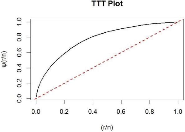
Figure 3 Scaled TT plot for the considered dataset.

Table 6 The model fitting summary for the considered data set based on MLE

Models	MLE	$-\log L$	AIC	BIC	K-S Statistic	p-value
xgamma ($\theta )$	$\widehat{\theta }=0.0549$	113.023	228.171	229.307	0.07451	0.96040
Exponential$(\theta )$	$\widehat{\theta }=0.0138$	121.435	244.870	246.005	0.10303	0.71330
Gamma $(\alpha ,\beta )$	$\widehat{\alpha }=4.0260$	113.821	230.058	232.330	0.35945	0.83761
	$\widehat{\beta }=0.0557$
Exponentiated	$\widehat{\alpha }=0.4634$	113.966	231.383	233.654	0.07603	0.95301
xgamma$(\alpha ,\theta )$	$\widehat{\theta }=0.00278$
Inverse xgamma $(\theta )$	$\widehat{\theta }=1.9201$	113.523	229.931	231.067	0.07587	0.94566

Table 7 Progressively first failure censored data for considered dataset

Group Items	1	2	3	4	5	6	7	8
(i)	12.20*	23.56*	23.74*	25.87*	41.35	195	47.38	110
(ii)	146	31.98	127	112	43*	63.47*	140	119*
(iii)	169	133	68.46	159	55.46	130	94*	92
Group items	9	10	11	12	13	14	15
(i)	37*	78.26*	209	249*	281*	194	58.36*
(ii)	179	519	725*	173	817	155*	173
(iii)	432	84	633	81	319	74.47	84

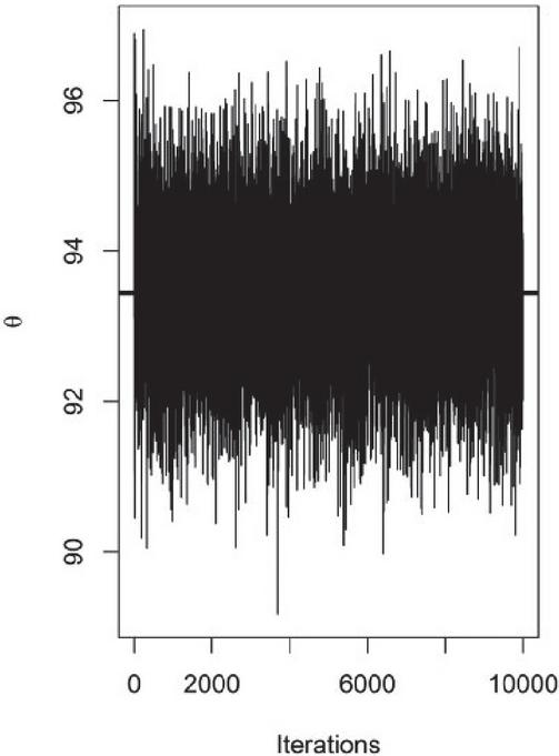
Figure 4 Trace plot of $\theta$.

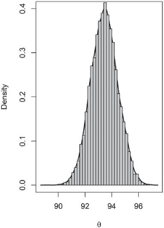
Figure 5 Histogram and density plot of $\theta$.

Now, the dataset has been divided into $n=15$ groups, each containing $k=3$ data points, after randomly assigning the data for the first-failure censored sample. In Table 7, the observations marked with an asterisk (*) indicate the first failure in each group. The final ordered list of first-failure censored data points is then provided as follows:

12.20, 23.56, 23.74, 25.87, 37, 41.35, 47.38, 58.36, 63.47, 74.47, 78.26, 81, 92, 209, 281

Finally, by implementing four distinct progressive censoring schemes on the previously obtained first-failure censored sample, with a set number of failures $m=10$, the resulting progressively first-failure censored samples for each scheme are presented as follows:

Scheme 1: $k=$ 3, $n=$ 15, $m=$ 10, $W=($5, 0*9),

$\underset{¯}{x}=[12.20,41.35,47.38,58.36,63.47,74.47,78.26,81,92,209]$

Scheme 2: $k=$ 3, $n=$ 15, $m=$ 10, $W=($1, 0*2, 1, 0*2, 2, 0*2, 1),

$\underset{¯}{x}=[12.20,23.74,25.87,37,41.35,47.38,58.36,78.26,81,92]$

Scheme 3: $k=$ 3, $n=$ 15, $m=$ 10, $W=($0*9, 5),

$\underset{¯}{x}=[12.20,23.56,23.74,25.87,37,41.35,47.38,58.36,63.47$, $74.47]$

Scheme 4: $k=$ 3, $n=$ 15, $m=$ 10, $W=($0*15),

$\underset{¯}{x}=[12.20,23.56,23.74,25.87,37,41.35,47.38,58.36,63.47$, $74.47,78.26,81,92,209,281]$

Table 8 ML and Bayes estimates of parameter and reliability characteristics under considered dataset for $k=3,n=15,m=10$

Scheme Parameters	Scheme 1	Scheme 2	Scheme 3	Scheme 4
$\widehat{\theta }$	96.345	83.766	72.178	73.107
${\theta }_{MH}^B$	94.345	81.256	71.024	72.154
$\widehat{R}\left(t\right)$	0.8003	0.9231	0.9265	0.8735
$R_L^B$	0.7960	0.9126	0.9216	0.8645
$R_{MH}^B$	0.7866	0.9171	0.9123	0.8659
$\widehat{h}\left(t\right)$	0.0075	0.0086	0.0087	0.0091
$h_L^B$	0.0076	0.0087	0.0087	0.0092
$h_{MH}^B$	0.0065	0.0078	0.0087	0.0089

Table 9 The 95% asymptotic and HPD credible intervals of parameter $\theta$ under considered real dataset

Scheme Parameters	Scheme 1	Scheme 2	Scheme 3	Scheme 4
${\widehat{\theta }}_{ACI}$	(72.48, 141.11)	(67.57, 117.86)	(62.19, 103.97)	(61.94, 100.26)
${\widehat{\theta }}_{HPD}$	(93.27, 98.26)	(77.67, 84.65)	(69.81, 76.13)	(69.90, 76.34)

Various censoring plans are employed to determine the ML and Bayesian estimates of the parameter $\theta$ as well as the associated reliability characteristics. These characteristics, including reliability $R(t)$ and hazard function $h(t)$ are calculated at the mission time $t$, which is defined as the median of the dataset. The Bayesian estimates for the parameter $\theta$ and the reliability characteristics are computed using a non-informative prior due to the lack of prior data. In this process, the Metropolis-Hastings algorithm is applied, generating 10,000 Markov chains, with the first 2,000 chains discarded as part of the burn-in period. Also, the 95% asymptotic and HPD credible intervals are calculated.

Point estimates for the parameter $\theta$ and reliability characteristics are summarized in Table 8, whereas Table 9 displays the interval estimates for $\theta$. The results for each censoring scheme are as follows:

• The estimates for the parameter $\theta$ across different estimation approaches are very similar and a comparable consistency is observed in the estimated values for other quantities, such as the reliability and hazard rate functions.

• Under each scheme, the HPD credible intervals are consistently shorter in length compared to the ACIs. This suggests that, for this dataset, the HPD method offers superior performance and efficiency.

• All reported confidence intervals indicate that the estimated value of the parameter $\theta$ could be any number greater than or equal to 61. This suggests that, based on the data, the lower bound of the parameter $\theta$ consistently exceeds 61 across all intervals.

8 Results and Conclusion

Reliability analysis is a cornerstone in understanding the performance and dependability of critical systems across diverse fields such as engineering, healthcare, and risk management. The demand for robust inferential procedures to estimate reliability parameters has grown significantly, especially for systems subject to complex censoring schemes. This study is motivated by the need to bridge the gap between classical and Bayesian approaches to parameter estimation, offering a comprehensive framework that integrates these paradigms for enhanced accuracy and applicability. By addressing the challenges of progressively first failure-censored data and leveraging modern computational techniques like the M-H algorithm, this work aims to contribute novel insights and tools to the evolving field of reliability modeling. This study develops and evaluates advanced inferential procedures for estimating the parameter $\theta$ and reliability characteristics of the xgamma model under progressively first failure-censored data. Both ML and Bayesian approaches are employed, with Bayesian estimation using the M-H algorithm to generate 10,000 Markov chains (after a burn-in of 2,000). Non-informative priors and asymptotic confidence intervals complement this analysis, with HPD credible intervals providing a robust measure of uncertainty. The findings demonstrate consistent estimates of $\theta$ and reliability characteristics across different censoring schemes. HPD intervals outperform asymptotic intervals, exhibiting superior precision and efficiency.

This work advances the field by employing the xgamma model under PFFCS, which provides greater flexibility and robustness in modeling real-world reliability data. Unlike previous research that predominantly emphasized point estimation, this study integrates maximum likelihood and Bayesian methods to deliver both point and interval estimates. Using advanced techniques like the Metropolis-Hastings algorithm, the Bayesian approach here offers higher precision, as demonstrated by the consistently shorter HPD credible intervals compared to asymptotic confidence intervals – an observation rarely addressed in prior work.

Additionally, while earlier studies often restricted their analyses to reliability and hazard functions under specific conditions, this research extends these evaluations to mission time, defined as the dataset median, and compares estimates across various censoring schemes. The xgamma model’s adaptability in handling progressively censored data addresses limitations in existing methodologies, making it particularly suitable for modern reliability applications. By combining rigorous numerical simulations with real-world data validation, this study not only reinforces the theoretical advancements but also underscores its practical utility. These contributions bridge critical gaps in the literature, offering a comprehensive framework for future research in reliability analysis using advanced censoring schemes.

This work provides a robust foundation for future advancements in reliability analysis. Potential avenues include extending the proposed methodologies to multidimensional and more complex reliability models, which could capture interactions among system components more effectively. Additionally, exploring alternative loss functions and prior distributions in the Bayesian framework may yield more context-specific estimators. The integration of these statistical approaches with emerging machine learning techniques offers a promising direction for improving both computational efficiency and predictive performance, particularly in big data environments. Moreover, the application of the developed methods to diverse censoring schemes and generalized lifetime distributions, such as hybrid or extended models, could broaden their utility across industries.

Conflict of Interest

There are not any potential conflicts of interests that are directly or indirectly related to the research.

Data Availability

The data that supports the findings of this study is available from the respective reference as mentioned in the main text.

References

Abu-Moussa, M., Alsadat, N., and Sharawy, A. (2023). On Estimation of Reliability Functions for the Extended Rayleigh Distribution under Progressive First-Failure Censoring Model. Axioms, 12(7): 680.

Balakrishnan, N., and Sandhu, R. (1995). A simple simulational algorithm for generating progressive type-II censored samples. The American Statistician, 49(2), 229–230.

Balasooriya, U. (1995). Failure–censored reliability sampling plans for the exponential distribution. Journal of Statistical Computation and Simulation, 52(4), 337–349.

Bi, Q., Ma, Y., and Gui, W. (2022). Reliability estimation for the bathtub-shaped distribution based on progressively first-failure censoring sampling. Communications in Statistics – Simulation and Computation, 51(8), 4564-4580.

Cohen, A. C. (1963). Progressively censored samples in life testing. Technometrics, 5(3), 327–339.

Chen, M. H., and Shao, Q. M. (1999). Monte Carlo estimation of Bayesian credible and HPD intervals. Journal of Computational and Graphical Statistics, 8(1), 69–92.

Dube, M., Garg, R., and Krishna, H. (2016). On progressively first failure censored Lindley distribution. Computational Statistics, 31, 139-163.

Efron, B. (1988). Logistic regression, survival analysis, and the Kaplan-Meier curve. Journal of the American Statistical Association, 83(402), 414–425.

Fathi, A., Farghal, A. A., and Soliman, A. A. (2022). Bayesian and Non-Bayesian Inference for Weibull Inverted Exponential Model under Progressive First-Failure Censoring Data. Mathematics, 10(10): 1648.

Gelman, A., Carlin, J. B., Stern, H. S., Dunson, D. B., Vehtari, A., and Rubin, D. B. (2013). Bayesian data analysis (3rd ed.). CRC Press.

Ghafouri, S., and Rastogi, M. K. (2021). Reliability analysis of Kumaraswamy distribution under progressive first-failure censoring. Journal of Statistical Modelling: Theory and Applications, 2(1), 67–99.

Hastings, W. K. (1970). Monte Carlo sampling methods using Markov chains and their applications. Biometrika, 57(1), 97–109.

Kumar, I., Kumar, K., and Ghosh, I. (2023). Reliability Estimation in Inverse Pareto Distribution Using Progressively First Failure Censored Data. American Journal of Mathematical and Management Sciences, 42(2), 126–147.

Lindley, D.V. (1980) Approximate bayesian methods.Trabajos de Estadística e Investigación Operativa, 31, 223–245.

Metropolis N., Rosenbluth A. W., Rosenbluth M. N., Teller A. H., and Teller E., (1953). Equation of State Calculations by Fast Computing Machines. The Journal of Chemical Physics, 21: 1087–1092.

Saini, S., Chaturvedi, A., and Garg, R. (2021). Estimation of stress–strength reliability for generalized Maxwell failure distribution under progressive first failure censoring. Journal of Statistical Computation and Simulation, 91(7), 1366–1393.

Sen, S., Chandra, N., and Maiti, S. (2018). Survival estimation in xgamma distribution under progressively type-II right censored scheme. Model Assisted Statistics and Applications, 13(2), 107–121.

Sen, S., Maiti, S., and Chandra, N. (2016). The xgamma Distribution: Statistical Properties and Application. Journal of Modern Applied Statistical Methods, 15(1), 774–788.

Wu, S.-J., and Kus, C. (2009). On estimation based on progressive first-failure-censored sampling. Computational Statistics & Data Analysis, 53(10), 3659–3670.

Yadav, A. (2023). Bayesian Estimation for Xgamma Distribution Under Type-I Hybrid Censoring Scheme Using Asymmetric Loss Function. Pakistan Journal of Statistics and Operation Research, 19(1), 27–49.

Yadav, A., Saha, M., Singh, S. K., and Singh, U. (2019). Bayesian Estimation of the Parameter and the Reliability Characteristics of xgamma Distribution Using Type-II Hybrid Censored Data. Life Cycle Reliability and Safety Engineering, 8, 1–10.

Zhang, F., and Gui, W. (2020). Parameter and Reliability Inferences of Inverted Exponentiated Half-Logistic Distribution under the Progressive First-Failure Censoring. Mathematics, 8(5): 708.

Biographies

Sunita Sharma is an Assistant Professor in the Department of Mathematics at Manipal Institute of Technology, Manipal, Karnataka. She holds a Ph.D. in Statistics from the Department of Mathematics, Statistics and Computer Science at G.B. Pant University of Agriculture and Technology, Pantnagar. Her research focuses on Bayesian estimation and reliability engineering. She has published extensively in reputed journals and serves as a reviewer for several esteemed academic publications. Dr. Sharma completed her B.Sc. and M.Sc. from Kumaun University, Nainital. Alongside her academic responsibilities, she remains actively engaged in research, contributing to advancements in her field.

Vinod Kumar is an esteemed Professor in the Department of Mathematics, Statistics, and Computer Science at G.B. Pant University of Agriculture and Technology, Pantnagar. With a distinguished career in academia, he has also held various administrative positions at the university. His research interests include Applied Statistics, Life Testing, Reliability and Bayesian Inference. He has published numerous research papers in reputed journals and actively contributes as a reviewer for many prestigious publications. Additionally, he serves as an Editor-in-Chief, further demonstrating his dedication to the advancement of statistical research.

Journal of Reliability and Statistical Studies, Vol. 18, Issue 1 (2025), 41–68.
doi: 10.13052/jrss0974-8024.1813
© 2025 River Publishers