Algorithms for Generating Neutrosophic Gamma Distributed Data
Muhammad Saleem1 and Muhammad Aslam2,*
1Department of Industrial Engineering, Faculty of Engineering, King Abdulaziz University, Rabigh, 21911, Saudi Arabia
2Department of Statistics, Faculty of Science, King Abdulaziz University, Jeddah 21589, Saudi Arabia
E-mail: msaleim1@kau.edu.sa; aslam_ravian@hotmail.com/magmuhammad@kau.edu.sa
*Corresponding Author
Received 26 February 2025; Accepted 28 June 2025
Abstract
The gamma distribution is well-known for its wide range of applications across various fields. Traditional gamma distributions and their associated algorithms have been used to model imprecise data; however, they face limitations in addressing uncertainty and indeterminacy. To overcome these challenges, this study introduces the neutrosophic gamma distribution, an extension of the classical gamma distribution that incorporates neutrosophic random variables to better handle imprecision and indeterminacy. Basic properties of the neutrosophic gamma distribution are presented, along with algorithms designed to generate data under different levels of indeterminacy. Simulation results reveal that as the degree of indeterminacy increases, the corresponding random variates tend to exhibit an upward trend. Comparative analysis with classical statistics highlights the significant effect of indeterminacy on data generation. Overall, the study demonstrates that the degree of indeterminacy plays a crucial role in shaping the behavior of data derived from the gamma distribution.
Keywords: Gamma distribution, random variate, indeterminacy, simulation, analysis.
1 Introduction
The gamma distribution is very important in reliability analysis, as shown in studies like [1] and [2]. In many cases, researchers use simulated data to support real data or when it’s difficult or impossible to collect real data that follows a gamma distribution. To create such data, special algorithms are used. These algorithms follow clear steps to simulate data based on specific conditions and parameters, helping ensure that the results match real-world situations as closely as possible. Simulating data using these algorithms is especially useful when collecting real data is too expensive or hard to do. Iriarte et al. [2] pointed out how useful it is to generate gamma-distributed random values in many different fields. The gamma distribution is also used in areas like Bayesian statistics and queuing theory, as shown in [3]. Other researchers have applied it in various fields – for example, Maaref and Annavajjala [4] in digital communications, Pati and Krishnan [5] in atmospheric studies, and Huber et al. [6] in economics. More details can be found in [7].
As mentioned earlier, generating random values from the gamma distribution is important in many fields. Gill [8] introduced one of the early methods for creating gamma random values. Atkinson and Pearce [9] developed algorithms for different types of statistical distributions, including the gamma distribution. Marsaglia and Tsang [10] proposed a simple and widely used method for generating gamma values. Robertson and Walls [11] provided algorithms for both the normal and gamma distributions. Tanizaki [12] created an algorithm that works for any shape parameter of the gamma distribution. Apolloni and Bassis [13] designed methods that use both parameters of the gamma distribution. Xi et al. [14] introduced a technique based on transformation to generate gamma values. Lawnik [15] explored how to simulate gamma data using an inverse chaotic transformation. Luengo [16] developed tools for generating pseudo-random gamma values.
The current algorithms for generating data from the gamma distribution are based on classical statistics and do not account for uncertainty or the degree of indeterminacy. Neutrosophic statistics, introduced by [17], is a modern approach designed to handle imprecise and uncertain data. Unlike classical methods, neutrosophic statistics includes a concept called the degree of indeterminacy, which classical statistics ignores. Neutrosophic statistics incorporates the degrees of truth, indeterminacy, and falsity, making it more informative than classical statistics. It reduces to classical statistical analysis when the degree of indeterminacy is absent. Methods for analyzing neutrosophic data have been presented by [18] and [19]. Smarandache [20] showed that neutrosophic statistics can be more effective than classical and interval-based approaches. Granados et al. [21] contributed by working on neutrosophic continuous distributions. Aslam [22] developed an algorithm to simulate neutrosophic data using the DUS-neutrosophic Weibull distribution, and later [23], introduced sine-cosine methods for generating neutrosophic data from the normal distribution. More examples of algorithms based on neutrosophic ideas can be found in [24] and [25]. Khan et al. [26] studied the neutrosophic gamma distribution and its use for complex data. Granados et al. [27] also introduced continuous distributions using neutrosophic random variables. Aslam and Alamri [28] created accept-reject-based algorithms for generating neutrosophic data from the uniform and Weibull distributions. Jdid et al. [29] proposed a method to convert uniform data into exponential data using neutrosophic statistics. In another study, Jdid et al. [30] developed algorithms to generate neutrosophic data from the gamma distribution. Aslam [31] also introduced the neutrosophic negative binomial distribution and its data generation methods, while Jdid and Smarandache [32] proposed a composition method to simulate neutrosophic data from the Poisson distribution. For more information on neutrosophic data generation algorithms, see references [22, 23, 33]. Alamri and Aslam [34] developed an algorithm for handling neutrosophic data based on the Erlang distribution.
The existing literature predominantly emphasizes classical statistical approaches to the gamma distribution, often overlooking the need for adaptable methodologies in uncertain environments. The gamma distribution under classical statistics and its associated algorithms are not equipped to effectively address indeterminacy, limiting their applicability in scenarios characterized by significant uncertainty. Although algorithms under classical statistics for generating random variates from the gamma distribution have been developed for certain environments, no existing work, to the best of our knowledge, explores algorithms using the neutrosophic gamma distribution with the accept-reject method. This study aims to address this gap and improve existing methods by introducing the neutrosophic gamma distribution and developing accept-reject-based algorithms that account for the degree of indeterminacy, thereby addressing the limitations of classical statistical approaches. The main contributions of the study are the introduction of the neutrosophic gamma distribution, the examination of its basic properties, and the development of algorithms for generating random variates using the accept-reject method under various conditions, with a particular focus on the role of indeterminacy. Simulation studies highlight the impact of increasing uncertainty on random variate generation, underscoring the need for more nuanced statistical modeling approaches. Comparative analyses with methods under classical statistics demonstrate the distinctiveness and applicability of the proposed algorithms under neutrosophic statistics in addressing uncertain scenarios effectively. Section 2 presents a brief introduction to the neutrosophic random variable. Section 3 presents the neutrosophic gamma distribution with some basic properties. Section 4 discusses the two proposed algorithms when . Section 5 discusses the simulation using the algorithm when . Section 6 discusses the comparative studies for both algorithms. Section 7 discusses the application of the proposed method. Section 8 discusses the limitations of the proposed method and Section 9 discusses the concluding remarks.
2 Neutrosophic Random Variable
In this section, we will first the neutrosophic random variable with some basic properties of expectation and variance. Let us define the neutrosophic random variable having two parts as follows
| (1) |
The first part, , is known as the determinate part and represents the random variable in classical statistics. The second part, , is referred to as the indeterminate part, where represents the degree of uncertainty. It is important to note that the neutrosophic random variable defined in Equation (1) is a generalization of the classical random variable, incorporating both determinate and precise values. The neutrosophic random variable reduces to when . Suppose has a mean of and a variance of . The expectation and variance of the neutrosophic random variable’s properties are then given by [31].
| (2) | |
| (3) |
3 Neutrosophic Gamma Distribution
In this section, we will introduce the neutrosophic gamma distribution using the neutrosophic random variable. Suppose that follows the neutrosophic gamma distribution, where follows the gamma distribution under classical statistics and be the indeterminate part. The neutrosophic probability density function (npdf) of the gamma distribution, characterized by parameters (shape parameter) and (scale parameter), is defined as follows:
| (4) |
It is important to note that the neutrosophic gamma distribution simplifies to the classical gamma distribution when .
Note that refers to the gamma function and is defined as follows:
| (5) |
If is a positive integer, the neutrosophic gamma function is equal to .
The expected value and the variance of the random variable follows the gamma distribution is expressed by
| (6) | |
| (7) |
By applying the expectation properties on a neutrosophic random variable , the expectation of a neutrosophic gamma-distributed random variable is expressed as
| (8) |
The neutrosophic variance for the neutrosophic gamma distribution is defined as:
| (9) |
For small values of , the variance in Equation (9) can be approximated as follows
| (10) |
4 The Proposed Algorithms of Gamma Distribution
In this segment, we introduce two algorithms employing the neutrosophic gamma distribution. The behavior of these algorithms is contingent upon the parameter . The initial algorithm, as outlined by Thomopoulo [35], will be presented when the values are below one. Conversely, the second algorithm, also derived from Thomopoulo [35], will be elucidated for scenarios where the values exceed one.
4.1 Algorithm when
This section outlines the development of a procedure for generating random number when , as per Thomopoulo [35] and Ahrens and Dieter [36]. The proposed algorithm employs the accept-reject method. It is important to note that follows the neutrosophic gamma distribution with , while adheres to the gamma distribution with any positive value of . The algorithm is executed as follows:
Step-1: Pre-fix the values of and set , where
Step-2: Generate two uniform random numbers and from the uniform distribution , calculate
if ; then go to step-4
if ; then go to step-3
Step-3:
if then set , go to step-5
if then set , go to step-2
Step-4:
if then set , go to step-5
if then set , go to step-2
Step-5: Return
The algorithm to generate random variates when is shown in Figure 1.
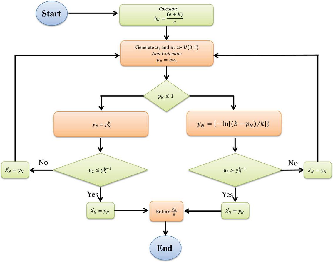
Figure 1 The algorithm to generate random variates when .
It is important to note that the proposed algorithm for the neutrosophic gamma distribution when extends the classical statistical algorithm. As illustrated in Figure 1, the proposed algorithm simplifies to the one presented by Thomopoulos [35] when no uncertainty is present in the data. Note that the neutrosophic mean given in Equation (8) and the approximate variance in Equation (10) were used to calculate the values of and , following the method outlined by Thomopoulos [35].
4.2 Algorithm when
This section outlines the development of a procedure for generating random number when , as per Thomopoulos [35] and Cheng [37]. The proposed algorithm employs the accept-reject method. It is important to note that follows the neutrosophic gamma distribution with , while adheres to the gamma distribution with any positive value of The algorithm is executed as follows:
Step-1: Pre-fix the values of and set ; ; ; and .
Step-2: Generate two uniform random numbers and from the uniform distribution , calculate ; ; and .
Step-3: if , then set , go to step-5
if , go to step-4
Step-4: if , then set , go to step-5
if , go to step-2.
Step-5: Return
The algorithm to generate random variates when is shown in Figure 2.
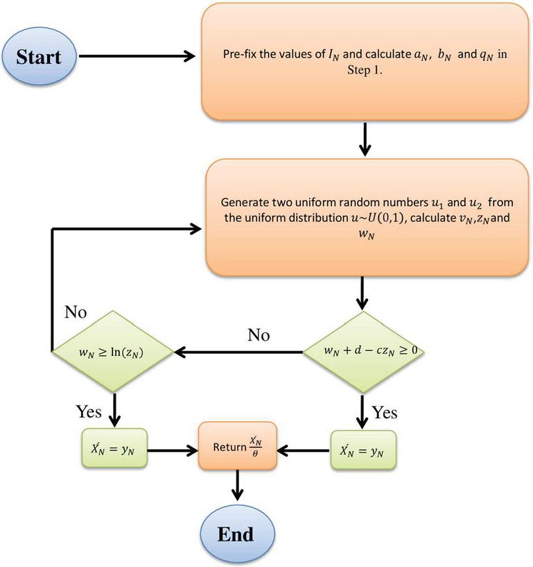
Figure 2 The algorithm to generate random variates when .
It is important to note that the proposed algorithm for the neutrosophic gamma distribution when extends the classical statistical algorithm. As illustrated in Figure 2, the proposed algorithm simplifies to the one presented by Thomopoulos [35] when no uncertainty is present in the data. Note that the neutrosophic mean given in Equation (8) and the approximate variance in Equation (10) were used to calculate the values of and , following the method outlined by Thomopoulos [35].
Table 1 Random numbers when and
| .1 | |||||||||
| 0.141 | 0.150 | 0.158 | 0.164 | 0.170 | 0.175 | 0.180 | 0.184 | 0.188 | 0.191 |
| 0.189 | 0.195 | 0.200 | 0.195 | 0.193 | 0.192 | 0.192 | 0.193 | 0.194 | 0.197 |
| 0.124 | 0.133 | 0.141 | 0.149 | 0.155 | 0.161 | 0.166 | 0.171 | 0.175 | 0.179 |
| 0.185 | 0.181 | 0.179 | 0.178 | 0.179 | 0.181 | 0.183 | 0.186 | 0.190 | 0.195 |
| 0.097 | 0.106 | 0.115 | 0.123 | 0.130 | 0.136 | 0.142 | 0.147 | 0.152 | 0.157 |
| 0.087 | 0.097 | 0.105 | 0.113 | 0.120 | 0.127 | 0.133 | 0.139 | 0.144 | 0.148 |
| 0.075 | 0.084 | 0.093 | 0.101 | 0.108 | 0.115 | 0.121 | 0.126 | 0.132 | 0.137 |
| 0.103 | 0.113 | 0.121 | 0.129 | 0.136 | 0.142 | 0.148 | 0.153 | 0.158 | 0.162 |
| 0.121 | 0.130 | 0.138 | 0.145 | 0.152 | 0.158 | 0.163 | 0.168 | 0.172 | 0.176 |
| 0.127 | 0.136 | 0.144 | 0.151 | 0.158 | 0.163 | 0.168 | 0.173 | 0.177 | 0.181 |
| 0.054 | 0.062 | 0.070 | 0.078 | 0.085 | 0.092 | 0.098 | 0.104 | 0.110 | 0.115 |
| 0.158 | 0.166 | 0.173 | 0.179 | 0.184 | 0.189 | 0.193 | 0.196 | 0.200 | 0.200 |
| 0.048 | 0.056 | 0.064 | 0.071 | 0.078 | 0.085 | 0.091 | 0.097 | 0.103 | 0.108 |
| 0.156 | 0.164 | 0.171 | 0.177 | 0.183 | 0.187 | 0.192 | 0.195 | 0.199 | 0.202 |
| 0.179 | 0.186 | 0.192 | 0.197 | 0.199 | 0.196 | 0.195 | 0.195 | 0.196 | 0.198 |
5 Simulation Using Algorithm when
In this section, we will showcase simulation studies conducted with the algorithm under the condition . We generated random variates from the gamma distribution, varying the mean, variance, , and values to analyze their impact on the data generated using the algorithm is presented in Figure 1. Table 1 displays results for a mean of 0.1, the variance of 0.02, of 0.5, and of 5. Likewise, Tables 2 and 3 present outcomes for different sets of parameters. For instance, Table 2 presents values corresponding to a mean of 0.05, the variance of 0.03, of 0.08, and of 1.67. Table 3 showcases results for a mean of 0.06, the variance of 0.04, of 0.09, and of 1.5. Analyzing Tables 1–3 reveals that as the degree of indeterminacy increases from 0.1 to 0.9, there is a general upward trend in the random variates. For instance, in Table 1, when , the random variate is 0.150, while for , it increases to 0.191. Figure 3 illustrates the trend in random variates when and , while Figures 4 and 5 depict the trends for with and with , respectively. Notably, Figures 3–5 show that as the values of increase, the random variates from the gamma distribution also increase. The curves corresponding to consistently occupy higher positions compared to other values. In conclusion, based on this simulation study, it is inferred that when , increasing the degree of uncertainty significantly influences the generation of random variates.
Table 2 Random numbers when and
| .1 | |||||||||
| 0.014 | 0.021 | 0.028 | 0.036 | 0.046 | 0.056 | 0.066 | 0.077 | 0.088 | 0.099 |
| 0.080 | 0.099 | 0.118 | 0.138 | 0.157 | 0.176 | 0.194 | 0.212 | 0.229 | 0.245 |
| 0.006 | 0.010 | 0.015 | 0.020 | 0.026 | 0.033 | 0.040 | 0.048 | 0.057 | 0.065 |
| 0.161 | 0.187 | 0.212 | 0.236 | 0.259 | 0.280 | 0.301 | 0.320 | 0.338 | 0.354 |
| 0.001 | 0.003 | 0.004 | 0.006 | 0.009 | 0.012 | 0.016 | 0.020 | 0.025 | 0.030 |
| 0.001 | 0.001 | 0.002 | 0.004 | 0.006 | 0.008 | 0.011 | 0.014 | 0.017 | 0.021 |
| 0.000 | 0.001 | 0.001 | 0.002 | 0.003 | 0.004 | 0.006 | 0.008 | 0.010 | 0.013 |
| 0.002 | 0.004 | 0.006 | 0.009 | 0.012 | 0.016 | 0.020 | 0.025 | 0.031 | 0.037 |
| 0.005 | 0.009 | 0.013 | 0.018 | 0.023 | 0.029 | 0.036 | 0.044 | 0.052 | 0.060 |
| 0.007 | 0.012 | 0.017 | 0.022 | 0.029 | 0.036 | 0.044 | 0.053 | 0.062 | 0.071 |
| 0.000 | 0.000 | 0.000 | 0.000 | 0.001 | 0.001 | 0.002 | 0.003 | 0.003 | 0.005 |
| 0.027 | 0.037 | 0.048 | 0.060 | 0.073 | 0.086 | 0.099 | 0.112 | 0.126 | 0.139 |
| 0.000 | 0.000 | 0.000 | 0.000 | 0.000 | 0.001 | 0.001 | 0.002 | 0.002 | 0.003 |
| 0.026 | 0.036 | 0.046 | 0.058 | 0.070 | 0.083 | 0.096 | 0.109 | 0.122 | 0.135 |
| 0.059 | 0.076 | 0.092 | 0.110 | 0.127 | 0.144 | 0.161 | 0.178 | 0.194 | 0.210 |
Table 3 Random numbers when and
| .1 | |||||||||
| 0.021 | 0.030 | 0.040 | 0.051 | 0.063 | 0.076 | 0.088 | 0.102 | 0.115 | 0.129 |
| 0.106 | 0.129 | 0.152 | 0.175 | 0.198 | 0.219 | 0.240 | 0.261 | 0.280 | 0.298 |
| 0.010 | 0.016 | 0.022 | 0.029 | 0.038 | 0.047 | 0.056 | 0.066 | 0.077 | 0.088 |
| 0.202 | 0.233 | 0.262 | 0.289 | 0.314 | 0.338 | 0.361 | 0.382 | 0.402 | 0.420 |
| 0.003 | 0.004 | 0.007 | 0.010 | 0.014 | 0.019 | 0.024 | 0.029 | 0.036 | 0.042 |
| 0.001 | 0.003 | 0.004 | 0.006 | 0.009 | 0.013 | 0.017 | 0.021 | 0.026 | 0.031 |
| 0.001 | 0.001 | 0.002 | 0.003 | 0.005 | 0.007 | 0.010 | 0.013 | 0.016 | 0.020 |
| 0.004 | 0.006 | 0.009 | 0.013 | 0.018 | 0.024 | 0.030 | 0.036 | 0.044 | 0.051 |
| 0.009 | 0.014 | 0.019 | 0.026 | 0.034 | 0.042 | 0.051 | 0.061 | 0.071 | 0.081 |
| 0.012 | 0.018 | 0.025 | 0.033 | 0.041 | 0.051 | 0.061 | 0.072 | 0.083 | 0.094 |
| 0.000 | 0.000 | 0.000 | 0.001 | 0.001 | 0.002 | 0.003 | 0.004 | 0.006 | 0.008 |
| 0.039 | 0.052 | 0.066 | 0.082 | 0.097 | 0.113 | 0.129 | 0.145 | 0.161 | 0.177 |
| 0.000 | 0.000 | 0.000 | 0.000 | 0.001 | 0.001 | 0.002 | 0.003 | 0.004 | 0.005 |
| 0.037 | 0.050 | 0.064 | 0.079 | 0.094 | 0.110 | 0.125 | 0.141 | 0.157 | 0.172 |
| 0.080 | 0.100 | 0.121 | 0.142 | 0.163 | 0.183 | 0.203 | 0.222 | 0.240 | 0.258 |
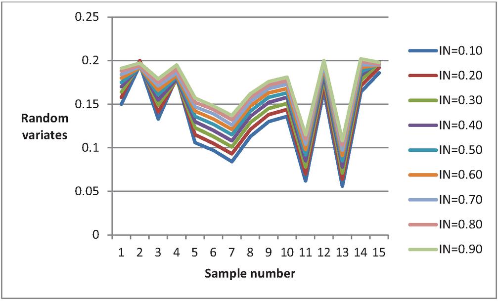
Figure 3 Random variates when and .
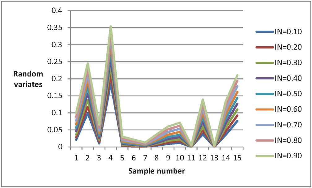
Figure 4 Random variates when and .
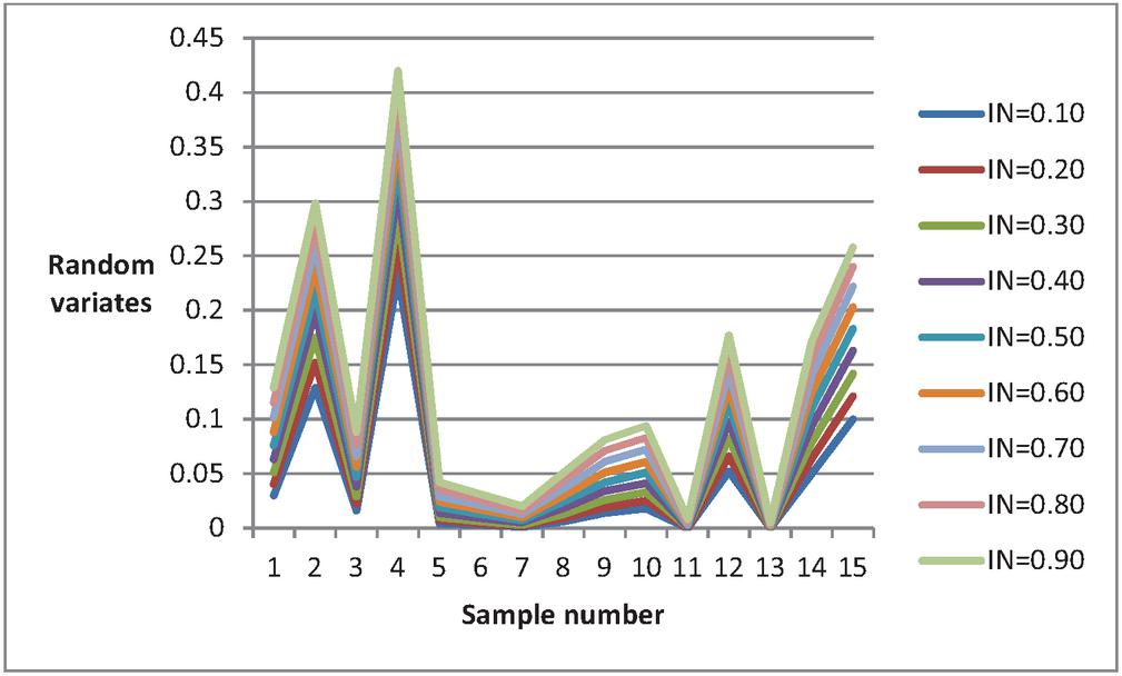
Figure 5 Random variates when and .
Table 4 Random numbers when and
| .1 | |||||||||
| 2.936 | 3.508 | 4.096 | 4.698 | 5.312 | 5.939 | 6.575 | 7.222 | 7.877 | 8.540 |
| 2.790 | 3.345 | 3.917 | 4.503 | 5.103 | 5.714 | 6.337 | 6.970 | 7.611 | 8.262 |
| 16.243 | 17.292 | 18.363 | 19.449 | 20.544 | 21.645 | 22.749 | 23.856 | 24.964 | 26.073 |
| 3.396 | 4.018 | 4.654 | 5.302 | 5.961 | 6.630 | 7.308 | 7.995 | 8.690 | 9.392 |
| 5.126 | 5.898 | 6.677 | 7.463 | 8.254 | 9.050 | 9.852 | 10.659 | 11.470 | 12.285 |
| 12.830 | 13.878 | 14.931 | 15.989 | 17.049 | 18.110 | 19.171 | 20.232 | 21.293 | 22.354 |
| 5.211 | 5.990 | 6.775 | 7.566 | 8.362 | 9.164 | 9.971 | 10.783 | 11.599 | 12.419 |
| 10.464 | 11.475 | 12.487 | 13.499 | 14.511 | 15.523 | 16.535 | 17.547 | 18.559 | 19.571 |
| 9.325 | 10.306 | 11.287 | 12.267 | 13.248 | 14.228 | 15.209 | 16.190 | 17.172 | 18.154 |
| 22.719 | 23.645 | 24.647 | 25.700 | 26.785 | 27.895 | 29.020 | 30.157 | 31.302 | 32.454 |
| 16.676 | 17.721 | 18.792 | 19.879 | 20.976 | 22.080 | 23.188 | 24.299 | 25.411 | 26.525 |
| 8.386 | 9.335 | 10.283 | 11.232 | 12.181 | 13.131 | 14.082 | 15.033 | 15.985 | 16.939 |
| 21.712 | 22.666 | 23.687 | 24.750 | 25.843 | 26.955 | 28.081 | 29.217 | 30.361 | 31.508 |
| 10.000 | 11.000 | 12.000 | 13.000 | 14.000 | 15.000 | 16.000 | 17.000 | 18.000 | 19.000 |
| 1.579 | 1.967 | 2.377 | 2.806 | 3.253 | 3.716 | 4.192 | 4.682 | 5.185 | 5.698 |
6 Simulation Using Algorithm when
In this section, we will showcase simulation studies conducted with the algorithm under the condition . We generated random variates from the gamma distribution, varying the mean, variance, , and values to analyze their impact on the data generated using the algorithm is presented in Figure 2. Table 4 displays results for a mean of 10, the variance of 66.6, of 1.5, and of 0.15. Likewise, Tables 5 and 6 present outcomes for different sets of parameters. For instance, Table 5 presents values corresponding to a mean of 12, the variance of 72, of 2.00, and of 0.17. Table 6 showcases results for a mean of 14, the variance of 65.4, of 3.00, and of 0.21. Analyzing Tables 4–6 reveals that as the degree of indeterminacy increases from 0.1 to 0.9, there is a general upward trend in the random variates. For instance, in Table 4, when , the random variate is 3.508, while for , it increases to 8.540. Figure 6 illustrates the trend in random variates when and , while Figures 7 and 8 depict the trends for with and with , respectively. Notably, Figures 6–8 show that as the values of increase, the random variates from the gamma distribution also increase. The curves corresponding to consistently occupy higher positions compared to other values. In conclusion, based on this simulation study, it is inferred that when , increasing the degree of uncertainty significantly influences the generation of random variates.
Table 5 Random numbers when and
| .1 | |||||||||
| 4.408 | 5.153 | 5.914 | 6.692 | 7.483 | 8.287 | 9.102 | 9.927 | 10.762 | 11.607 |
| 4.229 | 4.955 | 5.700 | 6.461 | 7.236 | 8.024 | 8.824 | 9.635 | 10.456 | 11.286 |
| 17.837 | 19.154 | 20.479 | 21.807 | 23.137 | 24.468 | 25.799 | 27.128 | 28.457 | 29.784 |
| 4.965 | 5.762 | 6.574 | 7.400 | 8.238 | 9.087 | 9.946 | 10.814 | 11.691 | 12.576 |
| 6.950 | 7.903 | 8.864 | 9.833 | 10.809 | 11.791 | 12.780 | 13.774 | 14.773 | 15.777 |
| 14.710 | 15.982 | 17.256 | 18.529 | 19.803 | 21.075 | 22.347 | 23.617 | 24.887 | 26.155 |
| 7.045 | 8.004 | 8.971 | 9.946 | 10.927 | 11.915 | 12.909 | 13.909 | 14.913 | 15.922 |
| 12.453 | 13.668 | 14.882 | 16.096 | 17.310 | 18.524 | 19.738 | 20.951 | 22.164 | 23.377 |
| 11.334 | 12.511 | 13.688 | 14.865 | 16.043 | 17.222 | 18.400 | 19.580 | 20.759 | 21.939 |
| 23.463 | 24.781 | 26.128 | 27.494 | 28.872 | 30.258 | 31.648 | 33.042 | 34.436 | 35.831 |
| 18.224 | 19.545 | 20.874 | 22.207 | 23.543 | 24.879 | 26.216 | 27.551 | 28.886 | 30.219 |
| 10.392 | 11.532 | 12.672 | 13.814 | 14.958 | 16.102 | 17.248 | 18.395 | 19.543 | 20.693 |
| 22.610 | 23.934 | 25.282 | 26.647 | 28.022 | 29.402 | 30.787 | 32.173 | 33.561 | 34.948 |
| 12.000 | 13.200 | 14.400 | 15.600 | 16.800 | 18.000 | 19.200 | 20.400 | 21.600 | 22.800 |
| 2.655 | 3.201 | 3.770 | 4.360 | 4.970 | 5.596 | 6.238 | 6.895 | 7.565 | 8.247 |
Table 6 Random numbers when and
| .1 | |||||||||
| 6.442 | 7.396 | 8.367 | 9.354 | 10.355 | 11.369 | 12.394 | 13.430 | 14.475 | 15.529 |
| 6.238 | 7.174 | 8.129 | 9.099 | 10.085 | 11.083 | 12.093 | 13.115 | 14.146 | 15.186 |
| 19.034 | 20.586 | 22.137 | 23.685 | 25.230 | 26.772 | 28.312 | 29.849 | 31.383 | 32.914 |
| 7.065 | 8.069 | 9.090 | 10.124 | 11.171 | 12.229 | 13.297 | 14.375 | 15.461 | 16.555 |
| 9.169 | 10.324 | 11.488 | 12.661 | 13.841 | 15.028 | 16.222 | 17.421 | 18.625 | 19.835 |
| 16.393 | 17.876 | 19.358 | 20.837 | 22.315 | 23.790 | 25.264 | 26.736 | 28.207 | 29.676 |
| 9.265 | 10.426 | 11.596 | 12.775 | 13.960 | 15.153 | 16.352 | 17.556 | 18.765 | 19.980 |
| 14.408 | 15.824 | 17.239 | 18.654 | 20.068 | 21.482 | 22.896 | 24.309 | 25.722 | 27.135 |
| 13.394 | 14.770 | 16.146 | 17.523 | 18.900 | 20.278 | 21.657 | 23.036 | 24.416 | 25.796 |
| 23.541 | 25.164 | 26.791 | 28.419 | 30.045 | 31.670 | 33.292 | 34.911 | 36.527 | 38.139 |
| 19.354 | 20.913 | 22.471 | 24.026 | 25.578 | 27.128 | 28.674 | 30.218 | 31.759 | 33.297 |
| 12.523 | 13.860 | 15.200 | 16.541 | 17.884 | 19.228 | 20.575 | 21.922 | 23.271 | 24.621 |
| 22.875 | 24.491 | 26.110 | 27.728 | 29.345 | 30.960 | 32.571 | 34.180 | 35.786 | 37.388 |
| 14.000 | 15.400 | 16.800 | 18.200 | 19.600 | 21.000 | 22.400 | 23.800 | 25.200 | 26.600 |
| 4.349 | 5.103 | 5.880 | 6.679 | 7.498 | 8.334 | 9.186 | 10.053 | 10.934 | 11.827 |
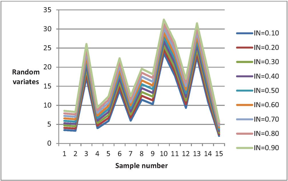
Figure 6 Random variates when , and .
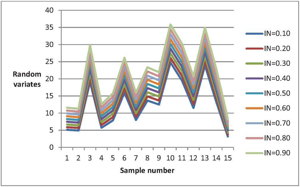
Figure 7 Random variates when , and .
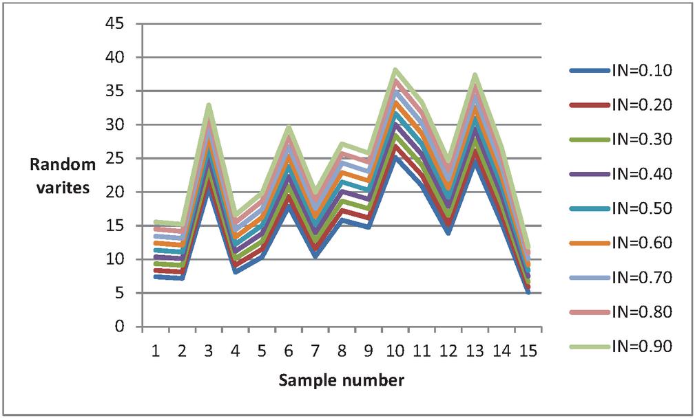
Figure 8 Random variates when , and .
7 Comparative Studies
As previously mentioned, neutrosophic statistics serve as an extension of classical statistics. Consequently, the algorithms proposed within neutrosophic statistics converge to their classical counterparts when equal to zero. In order to assess the outcomes of the proposed algorithms against those introduced by Thomopoulos [35], random variates sourced from the gamma distribution are generated. The results are organized in Tables 1–3 for scenarios where is less than 1. For cases where is greater than or equal to 1, the random variates derived using classical statistics are presented in Tables 4–6. Our analysis will initially focus on comparing the two algorithms when is less than 1, followed by a comparison when is greater than or equal to 1.
7.1 Comparative Study when
We now examine the random number generation using both the proposed and existing algorithms within the framework of classical statistics as presented in Thomopoulos [35], with specific values assigned to and . The results are compared by illustrating the random variates curves generated by the two algorithms in Figure 9. The upper curve depicts the random variate curve for , whereas the lower curve represents values of random variates for as described in Thomopoulos [35]. Analysis of Figure 9 reveals an increase in random variates as the degree of indeterminacy rises. Notably, the existing algorithm, operating under classical statistics, produces smaller values of random variates, as depicted in the figure. This observation underscores the influence of the degree of indeterminacy on random number generation from the gamma distribution in uncertain environments. Consequently, it is recommended to account for the degree of uncertainty when utilizing random numbers in practical applications.
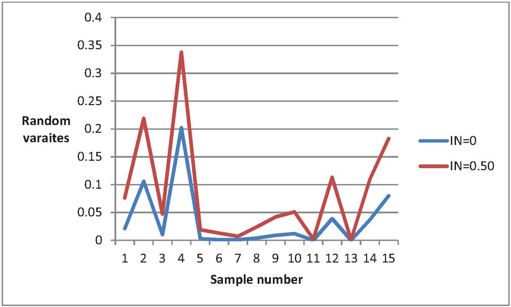
Figure 9 Random variates when and .
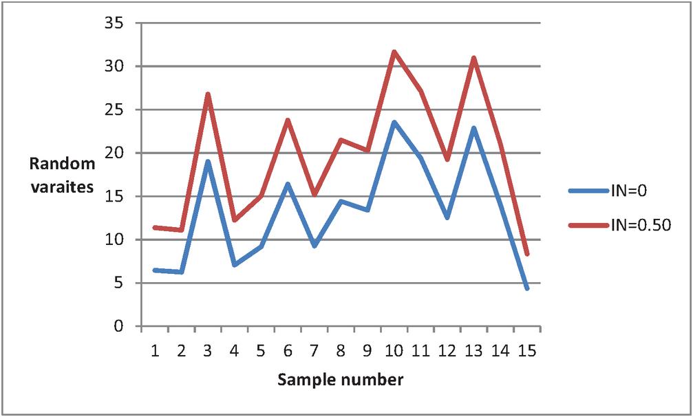
Figure 10 Random variates when , and .
7.2 Comparative Study when
Presently, we investigate the random number generation using both the proposed and existing algorithms within the framework of classical statistics as presented in Thomopoulos [35], with specific values assigned to and . The obtained results are compared by depicting the random variates curves generated by the two algorithms in Figure 10. The upper curve illustrates the random variate curve for , while the lower curve represents values of random variates for as mentioned in Thomopoulos [35]. An examination of Figure 10 reveals an increase in random variates as the degree of indeterminacy rises. Significantly, the existing algorithm, functioning under classical statistics, yields smaller values of random variates, as portrayed in the figure. To further understand the behavior of random variates with varying values, Figure 11 is presented, showcasing the random variates’ response as transitions from 1.5 to 3. Figure 11 clearly demonstrates an ascending trend in random variates as the values of increase. This finding emphasizes the impact of the degree of indeterminacy on random number generation from the gamma distribution in uncertain environments. Consequently, it is advisable to consider the degree of uncertainty when incorporating random numbers into practical applications.
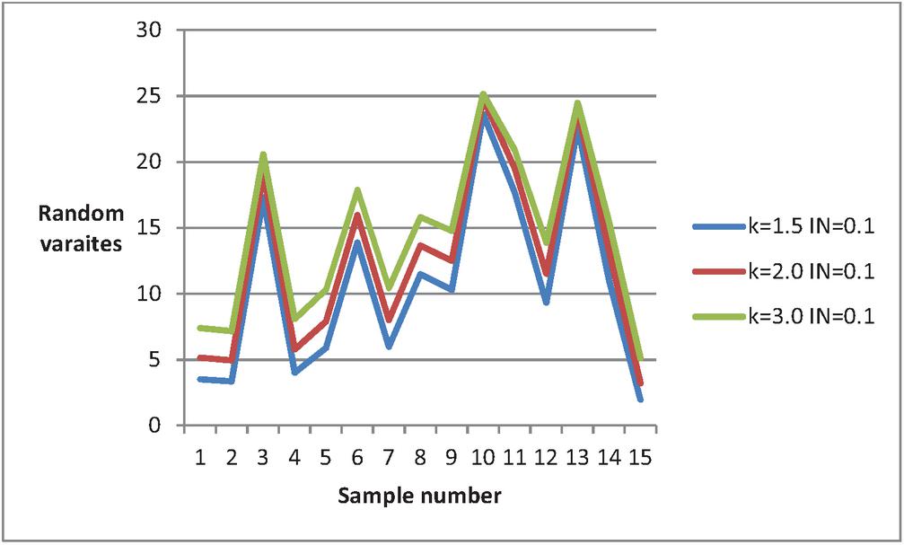
Figure 11 Random variates curves for various .
8 Application in Acceptance Sampling Plan
This section presents the application of neutrosophic data following the neutrosophic gamma distribution in the area of acceptance sampling plans. Acceptance sampling is widely used for product testing and inspection, particularly when failure times are modeled by a gamma distribution. Previous studies, such as those by [38–40], demonstrate the design of acceptance sampling plans using gamma-distributed failure times. However, failure time data is often imprecise, and neutrosophic statistics can capture this inherent uncertainty. Here, we compare acceptance sampling plans under two scenarios: with uncertainty (neutrosophic parameters) and without it. In acceptance sampling, the acceptance number and sample size are key parameters. Testing is conducted over a fixed duration , and the lot is accepted if the number of failures is less than within that time; otherwise, it is rejected. For illustration, we assume , , and hours, with product failure times following a gamma distribution where and . Table 5 shows failure times under two uncertainty levels: when (no uncertainty) and (some uncertainty), enabling comparison of plan effectiveness in handling imprecise data.
0: 2.655, 4.229, 4.408, 4.965, 6.95, 7.045, 10.392, 11.334, 12, 12.453, 14.71, 17.837, 18.224, 22.61, 23.463
0.1: 3.201, 4.955, 5.153, 5.762, 7.903, 8.004, 11.532, 12.511, 13.2, 13.668, 15.982, 19.154, 19.545, 23.934, 24.781
Using a gamma distribution under classical statistics, a product lot will be accepted if fewer than 2 failures occur within 5 hours. In this case, the analysis shows 4 failures within this period, leading to a lot of rejection. However, applying the proposed neutrosophic gamma distribution to the same data reveals only 2 failures within 5 hours, resulting in lot acceptance. This comparison highlights how assuming precise versus imprecise failure times can impact decisions about the product lot. Consequently, incorporating degrees of uncertainty is recommended when using acceptance sampling plans with a gamma distribution, as this approach accommodates indeterminacy in failure times, providing a more flexible and potentially accurate decision-making process.
9 Utilization, Assumptions and Limitations
The comparative analysis of simulation studies reveals distinguishable differences in the random variates generated from classical statistics and those under neutrosophic statistics. The findings underscore the significant impact of the degree of indeterminacy on random variate generation. Consequently, it is recommended to update computer software using the proposed algorithm for generating random variates from the gamma distribution. To account for the degree of indeterminacy, the existing algorithms in computer systems should be revised accordingly. However, it is important to note that the proposed algorithm has limitations and makes certain assumptions. Specifically, it is designed solely for generating gamma variates, and it is not applicable for obtaining normal variates. Moreover, the proposed algorithm is not suitable for scenarios where there is no uncertainty present in the data.
10 Concluding Remarks
In conclusion, this study introduced the neutrosophic gamma distribution as a valuable extension of classical statistics, enabling the handling of uncertainty and indeterminacy. Additionally, we proposed two algorithms for generating neutrosophic data from the gamma distribution. These algorithms effectively produced random variates under varying conditions, highlighting distinct trends influenced by the degree of indeterminacy. Simulation studies illustrated how increasing uncertainty impacts random variate generation. For example, analyzing Tables 1–3 shows a general upward trend in random variates as the degree of indeterminacy () increases from 0.1 to 0.9. Specifically, in Table 1, when , the random variate is 0.150, while at , it rises to 0.191. Furthermore, the proposed method was applied to an acceptance sampling plan. Under the classical gamma distribution, a lot was rejected with four failures in five hours. However, using the neutrosophic gamma distribution, the lot was accepted with only two failures, showcasing the practical advantages of the proposed approach in decision-making under uncertainty. The comparative analyses with classical statistics underscored the significance of accounting for indeterminacy, highlighting the limitations of traditional methods in uncertain environments. This study is significant as it addresses the increasing need to update existing statistical methods to effectively handle the degree of uncertainty commonly encountered in practice. Recommendations included updating computer software using the proposed algorithm and acknowledging the degree of uncertainty in practical applications. While the proposed algorithms showed promise, it was crucial to recognize their limitations, particularly in their applicability only to gamma variates and not normal variates. These findings contributed to the evolving landscape of statistical methodologies, encouraging further research into adapting statistical tools to better accommodate uncertainty. Overall, this study paves the way for future research into the practical applications and broader implications of the neutrosophic gamma distribution across various fields, such as statistical process control and reliability analysis. Developing specialized software and adapting existing modules to incorporate the proposed algorithms represents a valuable direction for future work. Moreover, an in-depth exploration of the statistical properties of the neutrosophic gamma distribution offers a promising avenue for further investigation and theoretical advancement.
Declarations
Ethics Approval and Consent to Participate
Not applicable.
Consent for Publication
Not applicable.
Availability of Data and Materials
The data is given in the paper.
Competing Interests
The authors declare no conflict of interest.
Authors’ Contributions
M.S and M.A wrote the paper.
Funding
No funds for the paper.
Acknowledgements
The authors are deeply thankful to the editor and reviewers for their valuable suggestions to improve the quality and personation of the paper. We acknowledge the use of ChatGPT to improve the clarity and grammar of the manuscript’s English language.
References
[1] Eric, U., O.M.O. Olusola, and F.C. Eze, A Study of Properties and Applications of Gamma Distribution. Statistics, 2020. 4(2): p. 52–65.
[2] Iriarte, Y.A., et al., A Gamma-Type distribution with applications. Symmetry, 2020. 12(5): p. 870.
[3] Brown, P.J. and J.E. Griffin, Inference with normal-gamma prior distributions in regression problems. 2010. 5 (1): p. 171–188.
[4] Maaref, A. and R. Annavajjala, The gamma variate with random shape parameter and some applications. IEEE communications letters, 2010. 14(12): p. 1146–1148.
[5] Pati, P.S. and P. Krishnan, Modelling of OFDM based RoFSO system for 5G applications over varying weather conditions: A case study. Optik, 2019. 184: p. 313–323.
[6] Huber, F., G. Koop, and L. Onorante, Inducing sparsity and shrinkage in time-varying parameter models. Journal of Business & Economic Statistics, 2021. 39(3): p. 669–683.
[7] Plubin, B. and P. Siripanich, An alternative goodness-of-fit test for a gamma distribution based on the independence property. Chiang Mai J Sci, 2017. 44(3): p. 1180–1190.
[8] Gill, D.J., The Generation of Pseudo Random Numbers from the Gamma Distribution, 1963, Ohio State University.
[9] Atkinson, A. and M. Pearce, The computer generation of beta, gamma and normal random variables. Journal of the Royal Statistical Society: Series A (General), 1976. 139(4): p. 431–448.
[10] Marsaglia, G. and W.W. Tsang, A simple method for generating gamma variables. ACM Transactions on Mathematical Software (TOMS), 2000. 26(3): p. 363–372.
[11] Robertson, I. and L. Walls, Random number generators for the normal and gamma distributions using the ratio of uniforms method, 1980, CM-P00068658.
[12] Tanizaki, H., A simple gamma random number generator for arbitrary shape parameters. Economics Bulletin, 2008. 3(7): p. 1–10.
[13] Apolloni, B. and S. Bassis, Algorithmic inference of two-parameter gamma distribution. Communications in Statistics-Simulation and Computation, 2009. 38(9): p. 1950–1968.
[14] Xi, B., K.M. Tan, and C. Liu, Logarithmic transformation-based gamma random number generators. Journal of Statistical Software, 2013. 55: p. 1–17.
[15] Lawnik, M., Generation of pseudo-random numbers with the use of inverse chaotic transformation. Open Mathematics, 2018. 16(1): p. 16–22.
[16] Luengo, E.A., Gamma Pseudo Random Number Generators. ACM Computing Surveys, 2022. 55(4): p. 1–33.
[17] Smarandache, F., Introduction to neutrosophic statistics: Infinite Study. Romania-Educational Publisher, Columbus, OH, USA, 2014.
[18] Chen, J., J. Ye, and S. Du, Scale effect and anisotropy analyzed for neutrosophic numbers of rock joint roughness coefficient based on neutrosophic statistics. Symmetry, 2017. 9(10): p. 208.
[19] Chen, J., et al., Expressions of rock joint roughness coefficient using neutrosophic interval statistical numbers. Symmetry, 2017. 9(7): p. 123.
[20] Smarandache, F., Neutrosophic Statistics is an extension of Interval Statistics, while Plithogenic Statistics is the most general form of statistics (second version). International Journal of Neutrosophic Science, 2022. 19(1): p. 148–165.
[21] Granados, C., A.K. Das, and D.A.S. Birojit, Some continuous neutrosophic distributions with neutrosophic parameters based on neutrosophic random variables. Advances in the Theory of Nonlinear Analysis and its Application, 2022. 6(3): p. 380–389.
[22] Aslam, M., Truncated variable algorithm using DUS-neutrosophic Weibull distribution. Complex & Intelligent Systems, 2023. 9(3): p. 3107–3114.
[23] Aslam, M., Simulating imprecise data: sine–cosine and convolution methods with neutrosophic normal distribution. Journal of Big Data, 2023. 10(1): p. 143.
[24] Guo, Y. and A. Sengur, NCM: Neutrosophic c-means clustering algorithm. Pattern Recognition, 2015. 48(8): p. 2710–2724.
[25] Garg, H., Algorithms for single-valued neutrosophic decision making based on TOPSIS and clustering methods with new distance measure. Aims Mathematics, 2020. 5(3): p. 2671–2693.
[26] Khan, Z., et al., On statistical development of neutrosophic gamma distribution with applications to complex data analysis. Complexity, 2021. 2021(1): p. 3701236.
[27] Granados, C., A.K. Das, and B. Das, Some continuous neutrosophic distributions with neutrosophic parameters based on neutrosophic random variables. Advances in the Theory of Nonlinear Analysis and its Application, 2022. 6(3): p. 380–389.
[28] Aslam, M. and F.S. Alamri, Algorithm for generating neutrosophic data using accept-reject method. Journal of Big Data, 2023. 10(1): p. 175.
[29] Jdid, M., R. Alhabib, and A. Salama, The basics of neutrosophic simulation for converting random numbers associated with a uniform probability distribution into random variables follow an exponential distribution. Neutrosophic Sets and Systems, 2023. 53(1): p. 22.
[30] Jdid, M., F. Smarandache, and K. Al Shaqsi, Generating Neutrosophic Random Variables Based Gamma Distribution. Plithogenic Logic and Computation, 2024. 1: p. 16–20.
[31] Aslam, M., The neutrosophic negative binomial distribution: algorithms and practical application: accepted-August 2024. REVSTAT-Statistical Journal, 2024. https://revstat.ine.pt/index.php/REVSTAT/article/view/781.
[32] Jdid, M. and F. Smarandache, Generating Neutrosophic Random Variables Following the Poisson Distribution Using the Composition Method (The Mixed Method of Inverse Transformation Method and Rejection Method). Neutrosohic Sets and Systems, 2024. 64: p. 132–140.
[33] Aslam, M., Developing Novel Algorithms for Generating Inexact Data through Triangle Distribution. IEEE Transactions on Big Data, 2024. DOI: \nolinkurl10.1109/TBDATA.2024.3460529.
[34] Alamri, F.S. and M. Aslam, Data generation and application using the neutrosophic Erlang distribution. Journal of Big Data, 2025. 12(1): p. 48.
[35] Thomopoulos, N.T., Essentials of Monte Carlo simulation: Statistical methods for building simulation models. 2014: Springer.
[36] Ahrens, J.H. and U. Dieter, Computer methods for sampling from gamma, beta, poisson and bionomial distributions. Computing, 1974. 12(3): p. 223–246.
[37] Cheng, R., The generation of gamma variables with non-integral shape parameter. Journal of the Royal Statistical Society Series C: Applied Statistics, 1977. 26(1): p. 71–75.
[38] Lu, W. and T.-R. Tsai, Interval censored sampling plans for the gamma lifetime model. European Journal of Operational Research, 2009. 192(1): p. 116–124.
[39] Gupta, S.S. and S.S. Gupta, Gamma distribution in acceptance sampling based on life tests. Journal of the American Statistical Association, 1961. 56(296): p. 942–970.
[40] Lee, A.H., et al., Designing acceptance sampling plans based on the lifetime performance index under gamma distribution. The International Journal of Advanced Manufacturing Technology, 2021. 115: p. 3409–3422.
Biographies
Muhammad Saleem received the master’s degree in computer science & communications engineering from the University of Duisburg-Essen, Germany, and the Ph.D. degree in engineering from the University of Federal Armed Forces, Munich, Germany. He has more than 15 years of teaching, research, and administrative experience with the Department of Industrial Engineering, University of Duisburg-Essen, and King Abdulaziz University, Saudi Arabia. He is currently an Associate Professor with King Abdulaziz University. He is actively involved in curriculum development and accreditation processes of engineering programs. His research interests include industrial quality control, artificial intelligence, and engineering management.
Muhammad Aslam was the first to introduce the field of neutrosophic statistical quality control (NSQC) and is the founder of several key areas within neutrosophic statistics, including neutrosophic inferential statistics, advanced neutrosophic distribution theory, neutrosophic survey sampling, neutrosophic design of experiments, neutrosophic reliability analysis, and neutrosophic index numbers. His major contribution lies in the original development of a comprehensive neutrosophic statistical theory for inspection, inference, and process control. Prof. Aslam extended the foundational concepts of classical statistics to neutrosophic statistics, formally initiating this advancement in 2018.
Journal of Reliability and Statistical Studies, Vol. 18, Issue 2 (2025), 289–312.
doi: 10.13052/jrss0974-8024.1822
© 2025 River Publishers