Bivariate Normal Distribution for Indeterminacy: Characteristics and Data Generation Algorithm

Muhammad Aslam^1,* and Muhammad Saleem²

¹Department of Statistics, Faculty of Science, King Abdulaziz University, Jeddah 21589, Saudi Arabia
²Department of Industrial Engineering, Faculty of Engineering, King Abdulaziz University, Rabigh, 21911, Saudi Arabia
E-mail: aslam_ravian@hotmail.com/magmuhammad@kau.edu.sa; msaleim1@kau.edu.sa
*Corresponding Author

Received 22 July 2025; Accepted 19 November 2025

Abstract

The existing bivariate normal distribution and its related algorithms in classical statistics cannot account for the degree of indeterminacy when applied under uncertainty. To address this gap, the main objective of this manuscript is to introduce bivariate neutrosophic random variables and study their properties through expectation and variance. In this paper, we also propose the neutrosophic bivariate normal distribution along with some of its key properties. Furthermore, we develop an algorithm based on the proposed distribution to generate imprecise data. A detailed simulation is carried out to examine the effect of the degree of indeterminacy on the data. The comparative study reveals that the variates produced by the proposed algorithm differ from those generated by the existing algorithm. To demonstrate its practical use, we provide a numerical example applying the bivariate normal distribution. Based on the simulation, comparative study, and numerical example, we recommend incorporating the degree of indeterminacy when generating data from the bivariate normal distribution under uncertainty.

Keywords: Classical statistics, simulation, uncertainty, bivariate normal distribution, algorithm.

1 Introduction

The bivariate normal distribution, an extension of the conventional normal distribution, plays a pivotal role in calculating the joint probability of two random variables co-occurring. This distribution is applied with the underlying assumption that both random variables adhere to a normal distribution. Its versatile application spans various fields, serving as a powerful tool for solving real-world problems. Notably, [1] proposed an algorithm for generating truncated multivariate data, showcasing the distribution’s adaptability in handling complex datasets. In the realm of reliability analysis, [2] harnessed the bivariate normal distribution to enhance their analytical approach. Grover et al. [3] extended its utility by utilizing both multivariate and bivariate normal distributions to estimate the duration of diabetes, demonstrating the distribution’s efficacy in diverse medical applications. Similarly, [4] employed bivariate models to analyze nitrogen data, underscoring its significance in environmental studies. The exploration of bivariate distributions extends beyond conventional applications, as evidenced by [5], who delved into bimodal distributions, providing valuable insights into its potential applications. Additionally, [6] expanded the scope of the bivariate normal distribution by introducing related regression models, contributing to the evolving landscape of statistical modeling. In response to the global pandemic, Bulut and Korukoglu [7] utilized the bivariate normal distribution for the analysis of Covid-19 data, showcasing its relevance in contemporary challenges. These diverse applications underscore the significance of the bivariate normal distribution as a foundational statistical tool with far-reaching implications across various disciplines. Alsalafi et al. [8] studied the bivariate transmuted family of distributions, exploring its properties and applications. Lee et al. [9] proposed a general class of discrete bivariate distributions for the usual stochastic order. Gaber et al. [10] introduced bivariate extensions of the Fréchet and Burr-type XII distributions.

Neutrosophic statistics constitutes a branch within mathematical science dedicated to handling imprecise, fuzzy, and uncertain data through processes involving collection, presentation, analysis, and inference. Neutrosophic statistics provides insights into the degree of indeterminacy, an aspect not addressed in fuzzy statistics. For details on developments in fuzzy statistics, see Nedosekin [11]. Serving as an extension of classical statistics, neutrosophic statistics operates within uncertain environments, in contrast to classical statistics, which primarily analyzes data within well-defined and certain contexts. The details about the neutrosophic analysis can be seen in [12]. The efficiency of the neutrosophic statistics over the interval-statistics can be seen in [13]. The neutrosophic methods to analyze the neutrosophic data can be seen in [14] and [15]. The use of negative binomial distribution for the fuzzy data can be seen in [16]. The development of discrete and continuous distribution using the idea of neutrosophy can be seen in [17] and [18]. The application of the neutrosophic statistics for the analysis of social data can be seen in Alvaracín Jarrín et al. [19]. The extension of the Rayleigh distribution using the neutrosophic statistics can be seen in [20]. AlAita and Aslam [21] and [22] introduced the neutrosophic statistics in the area of design of experiment and rank set sampling method, respectively. Ahsan-ul-Haq [23] extended the Kumaraswamy distribution to neutrosophic Kumaraswamy distribution. Jumaa et al. [24] studied the neutrosophic Gompertz-inverse Burr-X distribution with applications. Yassen and Amin [25] investigated the neutrosophic Moyal distribution. Megha et al. [26] introduced the neutrosophic DUS-exponential distribution with application. More application of neutrosophic statistics can be seen in [27]. The development of algorithms to generate the imprecise data for various situations can be seen in [28–32], and [33].

After an extensive review of the existing literature and to the best of the author’s knowledge, there appears to be a notable absence of research focused on the neutrosophic bivariate normal distribution for analysis within uncertain contexts. To bridge this gap, our endeavor involves the introduction of the neutrosophic bivariate random variable, delineating its properties in detail. Drawing inspiration from the concept of neutrosophy, we will subsequently put forth the neutrosophic bivariate normal distribution and explore various properties associated with this innovative statistical framework. Furthermore, a novel algorithm will be proposed to effectively generate imprecise data, enhancing the adaptability of the neutrosophic bivariate normal distribution in handling uncertain scenarios. The presentation of tables containing data generated from this distribution will provide valuable insights into its practical application. In-depth simulation and comparative studies will be conducted to elucidate the impact of uncertainty on data generation within this novel framework. A numerical example will be presented to illustrate the application of the proposed distribution. In essence, we anticipate that the introduction of the proposed distribution and its accompanying algorithm will contribute to a heightened level of flexibility in analyzing uncertain data, addressing a crucial need within the realm of statistical analysis.

2 Neutrosophic Random Variables

Consider neutrosophic random variables $X_{1N}=X_{1L}+X_{1L}{I}_N$; $I_Nϵ[I_L,I_U]$ and $X_{2N}=X_{2L}+X_{2L}{I}_N$; $I_Nϵ[I_L,I_U]$, where the first values $X_{1L}$, $X_{2L}$ show the determinate random variables and $X_{1L}{I}_N$, $X_{2L}{I}_N$ denote the indeterminate part of these neutrosophic numbers. Also note that $I_Nϵ[I_L,I_U]$ be the degree of indeterminacy. Granados [17] explained that the degree of indeterminacy makes the neutrosophic logic as the extension of the fuzzy logic. We assume that $X_{1L}$ and $X_{2L}$ follows the normal distribution with means ${\mu }_1$ and ${\mu }_2$ and variances ${\sigma }_1^2$ and ${\sigma }_2^2$, respectively. The expectations of the neutrosophic random variables are derived as follows

$E(X_{1N})$	$=E(X_{1L}+X_{1L}{I}_N)=(1+I_N){\mu }_1$	(1)
$E(X_{2N})$	$=E(X_{2L}+X_{2L}{I}_N)=(1+I_N){\mu }_2$	(2)

The variance of the neutrosophic random variables are derived as follows

$\mathit{Var}(X_{1N})$	$={\sigma }_{1N}^2=\mathit{Var}(X_{1L}+X_{1L}{I}_N)={(1+I_N)}^2{\sigma }_1^2$	(3)
$\mathit{Var}(X_{2N})$	$={\sigma }_{2N}^2=\mathit{Var}(X_{2L}+X_{2L}{I}_N)={(1+I_N)}^2{\sigma }_2^2$	(4)

The standard deviation of the neutrosophic random variables are derived as follows

${\sigma }_{1N}$	$=(1+I_N){\sigma }_1$	(5)
${\sigma }_{2N}$	$=(1+I_N){\sigma }_2$	(6)

The covariance between these two neutrosophic random variables is as follows

$\mathit{Cov}(X_{1N},X_{2N})$

$=E(X_{1N}{X}_{2N})-E(X_{1N})E(X_{2N})$

(7)

The correlation between two neutrosophic random variables is given by

$${\rho }_N=\frac{\mathit{Cov}(X_{1N},X_{2N})}{{\sigma }_{1N}{\sigma }_{2N}}$$

(8)

3 Neutrosophic Bivariate Normal

In this section, we aim to illustrate the transformation from a bivariate normal distribution within classical statistics to a neutrosophic bivariate normal distribution through the incorporation of neutrosophic random variables $X_{1N}=X_{1L}+X_{1L}{I}_N$; $I_Nϵ[I_L,I_U]$ and $X_{2N}=X_{2L}+X_{2L}{I}_N$; $I_Nϵ[I_L,I_U]$. Introducing the envisioned neutrosophic bivariate normal distribution, it is designed to be applicable in situations where data is characterized by fuzziness or uncertainty. The formulation of this proposed neutrosophic bivariate normal distribution is expressed as follows:

$f(X_{1N},X_{2N})$
$={\displaystyle \frac{1}{2\pi (1+I_N){\sigma }_1(1+I_N){\sigma }_2\sqrt{1-{\rho }_N^2}}}$
$\times \exp \{-{\displaystyle \frac{1}{2(1-{\rho }_N^2)}}[{\left({\displaystyle \frac{(1+I_N)x_{1L}-(1+I_N){\mu }_1}{(1+I_N){\sigma }_1}}\right)}^2$
$-2{\rho }_N\left({\displaystyle \frac{(1+I_N)x_{1L}-(1+I_N){\mu }_1}{(1+I_N){\sigma }_1}}\right)$
$\times \left({\displaystyle \frac{(1+I_N)x_{2L}-(1+I_N){\mu }_2}{(1+I_N){\sigma }_2}}\right)$
$+{\left({\displaystyle \frac{(1+I_N)x_{2L}-(1+I_N){\mu }_2}{(1+I_N){\sigma }_2}}\right)}^2]\}$	(9)

where ${\mu }_1,{\mu }_2,{\sigma }_1,{\sigma }_2,{\rho }_N^2$ are the five parameters.

3.1 Neutrosophic Conditional Distributions

Now, we present the neutrosophic conditional distribution in this section. Let $X_1=X_{10}$, where $X_{10}$ denotes the observed value of $X_1$, since the conditional mean and variance depend on this observed value. Then, the conditional mean of $X_2$ is given by

${\mu }_{X_2|X_{10}}$	$=(1+I_N){\mu }_2+{\rho }_N^2((1+I_N){\sigma }_2/(1+I_N){\sigma }_1)((1+I_N)X_{10}$
	$-(1+I_N){\mu }_1)$	(10)

The corresponding neutrosophic variance is as follows

$${\sigma }_{X_2|X_1}^2={\sigma }_2^2{(1+I_N)}^2(1-{\rho }_N^2)$$

(11)

The associated normal distribution of $X_2$ given $X_{10}$ is given by

$$X_2|X_{10}\sim NN({\mu }_{X_2|X_{10}},{\sigma }_{X_2|X_1}^2)$$

Let $X_2=X_{20}$, where $X_{20}$ denotes the observed value of $X_2$, since the conditional mean and variance depend on this observed value. Then, the conditional mean of $X_1$ is given by

${\mu }_{X_1|X_{20}}$	$=(1+I_N){\mu }_1+{\rho }_N^2((1+I_N){\sigma }_1/(1+I_N){\sigma }_2)((1+I_N)X_{20}$
	$-(1+I_N){\mu }_2)$	(12)

The corresponding neutrosophic variance is given by

$${\sigma }_{X_1|X_2}^2={\sigma }_1^2{(1+I_N)}^2(1-{\rho }_N^2)$$

(13)

The associated normal distribution of $X_2$ given $X_{10}$ is given by

$$X_1|X_{20}\sim NN({\mu }_{X_1|X_{20}},{\sigma }_{X_1|X_2}^2)$$

Theorem 1: Let $X_{1N}$ and $X_{2N}$ be jointly neutrosophic random variables, then, the normal distribution of $U_N=X_{1N}+X_{2N}$ is $U_N\sim N((1+I_N)({\mu }_1+{\mu }_2),{(1+I_N)}^2({\sigma }_1^2+{\sigma }_2^2+2{\sigma }_1{\sigma }_2\rho ))$.

Proof: Using the properties of expectation, we have

$E(U_N)=E(X_{1N}+X_{2N})=E(X_{1N})+E(X_{2N})=(1+I_N)({\mu }_1+{\mu }_2)$

Using the properties of variance, we have

$\mathit{Var}(U_N)$	$=\mathit{Var}(X_{1N}+X_{2N})=\mathit{Var}(X_{1N})+\mathit{Var}(X_{2N})$
	$+2\mathit{Cov}(X_{1N},X_{1N})$
$\mathit{Var}(U_N)$	$={(1+I_N)}^2{\sigma }_1^2+{(1+I_N)}^2{\sigma }_2^2+2{(1+I_N)}^2{\sigma }_1{\sigma }_2\rho$
$\mathit{Var}(U_N)$	$={(1+I_N)}^2({\sigma }_1^2+{\sigma }_2^2+2{\sigma }_1{\sigma }_2\rho )$

Therefore,

$$U_N\sim N((1+I_N)({\mu }_1+{\mu }_2),{(1+I_N)}^2({\sigma }_1^2+{\sigma }_2^2+2{\sigma }_1{\sigma }_2\rho )).$$

Theorem 2: Let $z_{1N}$ and $z_{2N}$ are two independent having mean $0$ and variance 1.

Proof: We define $z_{1N}=\frac{X_{1N}-{\mu }_{1N}}{{\sigma }_{1N}}$ and $z_{2N}=\frac{X_{2N}-{\mu }_{2N}}{{\sigma }_{2N}}$.

The mean and variance of $z_{1N}$ is given by

$E(z_{1N})$	$={\displaystyle \frac{E(X_{1N}-{\mu }_{1N})}{{\sigma }_{1N}}}={\displaystyle \frac{E(X_{1L}+X_{1L}{I}_N)-(1+I_N){\mu }_1}{{\sigma }_1(1+I_N)}}=0$
$\mathit{Var}(z_{1N})$	$=\mathit{Var}\left({\displaystyle \frac{(X_{1N}-{\mu }_{1N})}{{\sigma }_{1N}}}\right)={\displaystyle \frac{{(1+I_N)}^2{\sigma }_1^2}{{(1+I_N)}^2{\sigma }_1^2}}=1$

The mean variance for $z_{2N}$ can be prove similarly.

Theorem 3: Let $z_{1N}$ and $z_{2N}$ are two independent having mean $0$ and variance 1. Define

$$X=\frac{(1+I_N)X_{1L}-(1+I_N){\mu }_1}{{\sigma }_1(1+I_N)}=z_{1N}$$

and

$$z_{2N}=\frac{(1+I_N)X_{2L}-(1+I_N){\mu }_2}{{\sigma }_2(1+I_N)}$$

and

$Y$	$=\rho {\displaystyle \frac{(1+I_N)X_{1L}-(1+I_N){\mu }_1}{{\sigma }_1(1+I_N)}}$
	$+\sqrt{1-{\rho }^2}\left({\displaystyle \frac{(1+I_N)X_{2L}-(1+I_N){\mu }_2}{{\sigma }_2(1+I_N)}}\right)$

show that $X$ and $Y$ are bivariate normal.

Proof: Note that $z_{1N}$ and $z_{2N}$ are neutrosophic normal and independent and the joint probability density function is given by

$f_{z_{1N}{z}_{2N}}(z_{1N},z_{2N})$	$=f_{z_{1N}}(z_{1N})f_{z_{2N}}(z_{2N})$
	$={\displaystyle \frac{1}{2\pi }}\exp \left\{{\displaystyle \frac{-1}{2}}[z_{1N}^2+z_{2N}^2]\right\}$
	$={\displaystyle \frac{1}{2\pi }}\exp \{{\displaystyle \frac{-1}{2}}[{\left({\displaystyle \frac{(1+I_N)X_{1L}-(1+I_N){\mu }_1}{{\sigma }_1(1+I_N)}}\right)}^2$
	$+{\left({\displaystyle \frac{(1+I_N)X_{2L}-(1+I_N){\mu }_2}{{\sigma }_2(1+I_N)}}\right)}^2]\}$

We need to show that $aX+bY$ is normal for all $a$ and $b$, we have

$aX+bY$	$=a{\displaystyle \frac{(1+I_N)X_{1L}-(1+I_N){\mu }_1}{{\sigma }_1(1+I_N)}}$
	$+b[\rho {\displaystyle \frac{(1+I_N)X_{1L}-(1+I_N){\mu }_1}{{\sigma }_1(1+I_N)}}$
	$+\sqrt{1-{\rho }^2}\left({\displaystyle \frac{(1+I_N)X_{2L}-(1+I_N){\mu }_2}{{\sigma }_2(1+I_N)}}\right)]$
	$=(a+b\rho ){\displaystyle \frac{(1+I_N)X_{1L}-(1+I_N){\mu }_1}{{\sigma }_1(1+I_N)}}$
	$+b\sqrt{1-{\rho }^2}\left({\displaystyle \frac{(1+I_N)X_{2L}-(1+I_N){\mu }_2}{{\sigma }_2(1+I_N)}}\right)$

We see that it is the linear combination of $z_{1N}$ and $z_{2N}$ and thus it is neutrosophic normal.

Theorem 4: Let $z_{1N}$ and $z_{2N}$ are two independent having mean $0$ and variance 1. Define

$$X=\frac{(1+I_N)X_{1L}-(1+I_N){\mu }_1}{{\sigma }_1(1+I_N)}=z_{1N}$$

and

$$z_{2N}=\frac{(1+I_N)X_{2L}-(1+I_N){\mu }_2}{{\sigma }_2(1+I_N)}$$

and

$Y$	$=\rho {\displaystyle \frac{(1+I_N)X_{1L}-(1+I_N){\mu }_1}{{\sigma }_1(1+I_N)}}$
	$+\sqrt{1-{\rho }^2}\left({\displaystyle \frac{(1+I_N)X_{2L}-(1+I_N){\mu }_2}{{\sigma }_2(1+I_N)}}\right)$

Then, the correlation between $z_{1N}$ and $Y$ is

$$\rho (z_{1N},Y)=\rho .$$

Proof: We know that $\mathit{Var}(X)=\mathit{Var}(z_{1N})=1$ and

$\mathit{Var}(Y)$	$={\rho }^2\mathit{Var}\left({\displaystyle \frac{(1+I_N)X_{1L}-(1+I_N){\mu }_1}{{\sigma }_1(1+I_N)}}\right)$
	$+(1-{\rho }^2)\mathit{Var}\left({\displaystyle \frac{(1+I_N)X_{2L}-(1+I_N){\mu }_2}{{\sigma }_2(1+I_N)}}\right)=1$

Therefore,

$\rho (X,Y)$	$=\mathit{Cov}(X,Y)$
	$=\mathit{Cov}({\displaystyle \frac{(1+I_N)X_{1L}-(1+I_N){\mu }_1}{{\sigma }_1(1+I_N)}},$
	$\rho {\displaystyle \frac{(1+I_N)X_{1L}-(1+I_N){\mu }_1}{{\sigma }_1(1+I_N)}}$
	$+\sqrt{(1-{\rho }^2)}\left({\displaystyle \frac{(1+I_N)X_{2L}-(1+I_N){\mu }_2}{{\sigma }_2(1+I_N)}}\right))$
	$=\rho \mathit{Cov}({\displaystyle \frac{(1+I_N)X_{1L}-(1+I_N){\mu }_1}{{\sigma }_1(1+I_N)}},$
	${\displaystyle \frac{(1+I_N)X_{1L}-(1+I_N){\mu }_1}{{\sigma }_1(1+I_N)}}$
	$+\sqrt{\left(1-{\rho }^2\right)}\mathit{Cov}({\displaystyle \frac{(1+I_N)X_{1L}-(1+I_N){\mu }_1}{{\sigma }_1(1+I_N)}},$
	${\displaystyle \frac{(1+I_N)X_{2L}-(1+I_N){\mu }_2}{{\sigma }_2(1+I_N)}}))$
$\rho (X,Y)$	$=\rho .1+\sqrt{(1-{\rho }^2)}.0=\rho$

4 The Proposed Algorithm

In this section, we will present the design of the proposed algorithm under neutrosophic statistics. The existing algorithm mentioned in [34] is used to generate bivariate normal data under certain environment. The existing algorithm is unable to generate the bivariate normal data by considering the degree of uncertainty. We will modify the existing algorithm to generate the neutrosophic data from the bivariate normal distribution. The following routine will be applied to generate imprecise pair of data $x_{1N}$ and $x_{2N}$ the proposed algorithm is given by

Step-1: Specify $I_N$ and $I_{N{x}_{10}}$.

Step-2: Generate a random standard normal variable $z_1$ from mean 0 and variance 1.

Step-3: A random variable $x_{1N}$ is computed by

$$x_{10}=\frac{z_1(1+I_N){\sigma }_1+(1+I_N){\mu }_1}{(1+I_{N{x}_{10}})}$$

(14)

Step-4: The conditional mean and variance of $x_{2N}$ becomes ${\mu }_{X_2|X_{10}}=(1+I_N){\mu }_2+{\rho }_N^2((1+I_N){\sigma }_2/(1+I_N){\sigma }_1)((1+I_{N{x}_{10}})X_{10}-(1+I_N){\mu }_1)$ and ${\sigma }_{X_2|X_1}^2={\sigma }_2^2{(1+I_N)}^2(1-{\rho }_N^2)$, respectively.

Step-5: Generate a random standard normal variable $z_2$ from mean 0 and variance 1.

Step-6: The random variable $x_{2N}$ is computed by $x_{20}={\mu }_{X_2|X_{10}}+z_2{\sigma }_{X_2|X_1}$.

Step-7: Return $(x_{10},x_{20})$.

Note that when $I_L$ is set to 0, the algorithm suggested here simplifies to the one outlined in [34]. The operational steps of the proposed algorithm are illustrated in Figure 1.

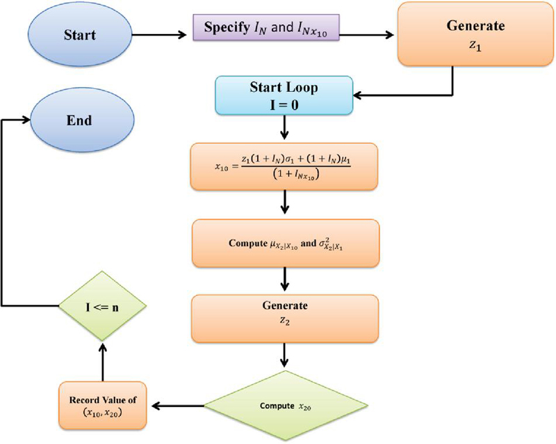
Figure 1 The propose algorithm.

5 Simulation Study

This section outlines the process of generating data from the bivariate normal distribution using the proposed algorithm. We explore the simulation procedure for generating data with various values of ${\mu }_1$, ${\mu }_2$, ${\sigma }_1^2$, ${\sigma }_2^2$, $\rho$, and $I_{N{x}_{10}}$. The resulting datasets are presented in Tables 1–4. Table 1 displays data from the bivariate normal distribution when ${\mu }_1=5$, ${\mu }_2=8$, ${\sigma }_1^2=1$, ${\sigma }_2^2=4$, $\rho =0.5$, and $I_{N{x}_{10}}=0.15$. Similarly, Table 2 presents data for the same parameters but with $I_{N{x}_{10}}=0.20$. Tables 3 and 4 exhibit data for ${\mu }_1=10$, ${\mu }_2=15$, ${\sigma }_1^2=1$, ${\sigma }_2^2=4$, $\rho =0.5$, and $I_{N{x}_{10}}=0.15$ and $I_{N{x}_{10}}=0.20$, respectively. Note that these parameters are set arbitrarily, and similar tables can be generated for other values. A pattern emerges in Tables 1–4, indicating an increasing trend in $(x_{10},x_{20})$ as $I_N$ varies from 0.1 to 0.5. For instance, with $I_N=0.1$, Table 1’s data (first row) is $(x_{10}=5.47,x_{20}=7.70)$, and with $I_N=0.2$, the data becomes ($x_{10}=5.97,x_{20}=8.60$). The influence of the degree of indeterminacy is further illustrated in Figures 2 and 3. These figures distinctly show that the curves of $(x_{10},x_{20})$ when $I_N=0.1$ are lower compared to other $I_N$ values. This study concludes that the degree of indeterminacy plays a significant role in the generation of bivariate normal data.

Table 1 Random variates from Algorithm when ${\mu }_1=5$, ${\mu }_2=8$, ${\sigma }_1^2=1$, ${\sigma }_2^2=4$, $\rho =0.5$, $I_{N{x}_{10}}=0.15$

$I_N=0$	$I_N=0.1$	$I_N=0.2$	$I_N=0.3$	$I_N=0.4$	$I_N=0.5$
$x_{10}$	$x_{20}$	$x_{10}$	$x_{20}$	$x_{10}$	$x_{20}$	$x_{10}$	$x_{20}$	$x_{10}$	$x_{20}$	$x_{10}$	$x_{20}$
5.72	6.85	5.47	7.70	5.97	8.60	6.47	9.55	6.96	10.56	7.46	11.62
4.53	5.66	4.33	6.11	4.72	6.54	5.12	6.93	5.51	7.28	5.90	7.60
5.04	6.17	4.82	6.79	5.26	7.42	5.69	8.05	6.13	8.68	6.57	9.32
3.41	4.54	3.26	4.62	3.55	4.60	3.85	4.47	4.15	4.21	4.44	3.82
4.40	5.53	4.21	5.95	4.60	6.32	4.98	6.66	5.36	6.95	5.74	7.18
4.22	5.35	4.04	5.71	4.41	6.01	4.77	6.26	5.14	6.45	5.51	6.57
5.89	7.02	5.64	7.93	6.15	8.90	6.66	9.93	7.17	11.03	7.69	12.21
5.40	6.53	5.17	7.28	5.64	8.05	6.11	8.86	6.58	9.69	7.05	10.56
5.74	6.87	5.49	7.73	5.99	8.64	6.49	9.60	6.99	10.62	7.49	11.70
3.47	4.60	3.32	4.71	3.62	4.72	3.93	4.61	4.23	4.39	4.53	4.04
6.65	7.78	6.36	8.94	6.94	10.20	7.52	11.59	8.09	13.10	8.67	14.76
4.97	6.09	4.75	6.70	5.18	7.30	5.61	7.89	6.04	8.49	6.48	9.08
6.20	7.32	5.93	8.33	6.46	9.42	7.00	10.59	7.54	11.86	8.08	13.23
5.37	6.50	5.13	7.23	5.60	7.99	6.07	8.78	6.53	9.59	7.00	10.44
3.57	4.70	3.42	4.84	3.73	4.89	4.04	4.83	4.35	4.66	4.66	4.38

Table 2 Random variates from Algorithm when ${\mu }_1=5$, ${\mu }_2=8$, ${\sigma }_1^2=1$, ${\sigma }_2^2=4$, $\rho =0.5$, $I_{N{x}_{10}}=0.20$

$I_N=0$	$I_N=0.1$	$I_N=0.2$	$I_N=0.3$	$I_N=0.4$	$I_N=0.5$
$x_{10}$	$x_{20}$	$x_{10}$	$x_{20}$	$x_{10}$	$x_{20}$	$x_{10}$	$x_{20}$	$x_{10}$	$x_{20}$	$x_{10}$	$x_{20}$
5.72	6.85	5.24	7.70	5.72	8.60	6.20	9.55	6.67	10.56	7.15	11.62
4.53	5.66	4.15	6.11	4.53	6.54	4.90	6.93	5.28	7.28	5.66	7.60
5.04	6.17	4.62	6.79	5.04	7.42	5.46	8.05	5.88	8.68	6.30	9.32
3.41	4.54	3.12	4.62	3.41	4.60	3.69	4.47	3.97	4.21	4.26	3.82
4.40	5.53	4.04	5.95	4.40	6.32	4.77	6.66	5.14	6.95	5.50	7.18
4.22	5.35	3.87	5.71	4.22	6.01	4.58	6.26	4.93	6.45	5.28	6.57
5.89	7.02	5.40	7.93	5.89	8.90	6.38	9.93	6.88	11.03	7.37	12.21
5.40	6.53	4.95	7.28	5.40	8.05	5.85	8.86	6.30	9.69	6.75	10.56
5.74	6.87	5.26	7.73	5.74	8.64	6.22	9.60	6.70	10.62	7.18	11.70
3.47	4.60	3.18	4.71	3.47	4.72	3.76	4.61	4.05	4.39	4.34	4.04
6.65	7.78	6.09	8.94	6.65	10.20	7.20	11.59	7.76	13.10	8.31	14.76
4.97	6.09	4.55	6.70	4.97	7.30	5.38	7.89	5.79	8.49	6.21	9.08
6.20	7.32	5.68	8.33	6.20	9.42	6.71	10.59	7.23	11.86	7.74	13.23
5.37	6.50	4.92	7.23	5.37	7.99	5.82	8.78	6.26	9.59	6.71	10.44
3.57	4.70	3.27	4.84	3.57	4.89	3.87	4.83	4.17	4.66	4.47	4.38

Table 3 Random variates from Algorithm when ${\mu }_1=10$, ${\mu }_2=15$, ${\sigma }_1^2=1$, ${\sigma }_2^2=4$, $\rho =0.5$, $I_{N{x}_{10}}=0.15$

$I_N=0$	$I_N=0.1$	$I_N=0.2$	$I_N=0.3$	$I_N=0.4$	$I_N=0.5$
$x_{10}$	$x_{20}$	$x_{10}$	$x_{20}$	$x_{10}$	$x_{20}$	$x_{10}$	$x_{20}$	$x_{10}$	$x_{20}$	$x_{10}$	$x_{20}$
10.72	13.85	10.25	15.40	11.19	17.00	12.12	18.65	13.05	20.36	13.98	22.12
9.53	12.66	9.11	13.81	9.94	14.94	10.77	16.03	11.60	17.08	12.43	18.10
10.04	13.17	9.60	14.49	10.47	15.82	11.35	17.15	12.22	18.48	13.09	19.82
8.41	11.54	8.04	12.32	8.77	13.00	9.50	13.57	10.23	14.01	10.96	14.32
9.40	12.53	8.99	13.65	9.81	14.72	10.63	15.76	11.45	16.75	12.27	17.68
9.22	12.35	8.82	13.41	9.62	14.41	10.43	15.36	11.23	16.25	12.03	17.07
10.89	14.02	10.42	15.63	11.37	17.30	12.31	19.03	13.26	20.83	14.21	22.71
10.40	13.53	9.95	14.98	10.86	16.45	11.76	17.96	12.67	19.49	13.57	21.06
10.74	13.87	10.27	15.43	11.21	17.04	12.14	18.70	13.08	20.42	14.01	22.20
8.47	11.60	8.10	12.41	8.84	13.12	9.58	13.71	10.31	14.19	11.05	14.54
11.65	14.78	11.14	16.64	12.15	18.60	13.17	20.69	14.18	22.90	15.19	25.26
9.97	13.09	9.53	14.40	10.40	15.70	11.27	16.99	12.13	18.29	13.00	19.58
11.20	14.32	10.71	16.03	11.68	17.82	12.66	19.69	13.63	21.66	14.60	23.73
10.37	13.50	9.92	14.93	10.82	16.39	11.72	17.88	12.62	19.39	13.52	20.94
8.57	11.70	8.20	12.54	8.95	13.29	9.69	13.93	10.44	14.46	11.18	14.88

Table 4 Random variates from Algorithm when ${\mu }_1=10$, ${\mu }_2=15$, ${\sigma }_1^2=1$, ${\sigma }_2^2=4$, $\rho =0.5$, $I_{N{x}_{10}}=0.20$

$I_N=0$	$I_N=0.1$	$I_N=0.2$	$I_N=0.3$	$I_N=0.4$	$I_N=0.5$
$x_{10}$	$x_{20}$	$x_{10}$	$x_{20}$	$x_{10}$	$x_{20}$	$x_{10}$	$x_{20}$	$x_{10}$	$x_{20}$	$x_{10}$	$x_{20}$
10.72	13.85	9.83	15.40	10.72	17.00	11.61	18.65	12.51	20.36	13.40	22.12
9.53	12.66	8.73	13.81	9.53	14.94	10.32	16.03	11.11	17.08	11.91	18.10
10.04	13.17	9.20	14.49	10.04	15.82	10.87	17.15	11.71	18.48	12.55	19.82
8.41	11.54	7.71	12.32	8.41	13.00	9.11	13.57	9.81	14.01	10.51	14.32
9.40	12.53	8.62	13.65	9.40	14.72	10.19	15.76	10.97	16.75	11.75	17.68
9.22	12.35	8.45	13.41	9.22	14.41	9.99	15.36	10.76	16.25	11.53	17.07
10.89	14.02	9.99	15.63	10.89	17.30	11.80	19.03	12.71	20.83	13.62	22.71
10.40	13.53	9.54	14.98	10.40	16.45	11.27	17.96	12.14	19.49	13.00	21.06
10.74	13.87	9.85	15.43	10.74	17.04	11.64	18.70	12.53	20.42	13.43	22.20
8.47	11.60	7.77	12.41	8.47	13.12	9.18	13.71	9.88	14.19	10.59	14.54
11.65	14.78	10.68	16.64	11.65	18.60	12.62	20.69	13.59	22.90	14.56	25.26
9.97	13.09	9.13	14.40	9.97	15.70	10.80	16.99	11.63	18.29	12.46	19.58
11.20	14.32	10.26	16.03	11.20	17.82	12.13	19.69	13.06	21.66	13.99	23.73
10.37	13.50	9.50	14.93	10.37	16.39	11.23	17.88	12.10	19.39	12.96	20.94
8.57	11.70	7.86	12.54	8.57	13.29	9.29	13.93	10.00	14.46	10.72	14.88

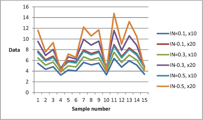
Figure 2 Data curves for various $I_N$ when ${\mu }_1=5$, ${\mu }_2=8$, ${\sigma }_1^2=1$, ${\sigma }_2^2=4$, $\rho =0.5,$ $I_{N{x}_{10}}=0.15$.

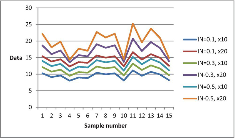
Figure 3 Data curves for various $I_N$ when ${\mu }_1=10$, ${\mu }_2$=15, ${\sigma }_1^2=1$, ${\sigma }_2^2=4$, $\rho =0.5,$ $I_{N{x}_{10}}=0.15$.

6 Comparative Study

The algorithm proposed for generating bivariate normally distributed data is an extension of [34]. When $I_L=0$, our proposed algorithm simplifies to the one outlined by [34]. To compare data from both algorithms, we present bivariate normal data using [34]’ algorithm in the first column of Tables 1–4. Our goal is to examine the impact of data generation under certain and uncertain environments. We present data from the bivariate normal distribution for both algorithms to observe the effect of the degree of indeterminacy on data generation. Tables 1–4 reveal differences between data generated from the bivariate normal distribution using the classical statistics algorithm by [34] and our proposed algorithm based on neutrosophic statistics. For instance, with $I_N=0$, Table 1’s data (first row) is ($x_{10}=5.72,x_{20}=6.85$), and with $I_N=0.3$, the data becomes ($x_{10}=6.47,x_{20}=9.55$). Figure 4 illustrates the behavior of bivariate normal distributed data from the proposed and existing algorithms. The curves of data from the existing algorithm in [34] differ significantly from those when $I_N=0.30$. The analysis concludes that the data generated using the existing algorithm varies considerably when generated under an indeterminate environment. This study emphasizes the importance of decision-makers exercising caution when utilizing [34] existing algorithm in uncertain environments.

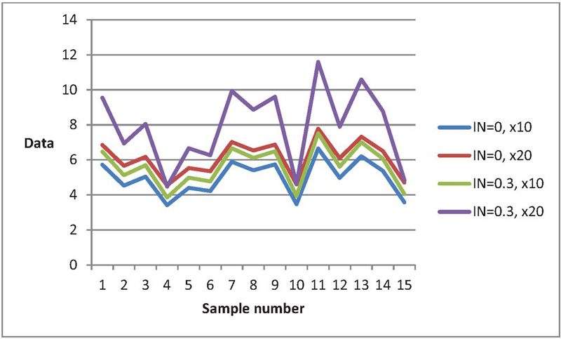
Figure 4 Data curves for the proposed algorithm and the existing algorithm when ${\mu }_1=5$, ${\mu }_2=8,$ ${\sigma }_1^2=1,$ ${\sigma }_2^2=4,$ $\rho =0.5,$ $I_{N{x}_{10}}=0.15$.

7 Example

Let $X_{1N}$ and $X_{2N}$ be jointly neutrosophic random variables with parameters ${\mu }_1=5$, ${\mu }_2=8$, ${\sigma }_1^2=1$, ${\sigma }_2^2=4$, $\rho =0.5$ and $I_N=0.1$. Find $P(X_{1N}+X_{2N}>0)$

Sol: Let $U_N=X_{1N}+X_{2N}$, then the mean of $U$ is given by

$E(U_N)$	$=E(X_{1N}+X_{2N})=E(X_{1N})+E(X_{2N})$
	$=(1+I_N){\mu }_1+(1+I_N){\mu }_2$
$E(U_N)$	$=(1+0.1)5+(1+0.1)8=14.3$
$\mathit{Var}(U_N)$	$=\mathit{Var}(X_{1N}+X_{2N})$
	$=\mathit{Var}(X_{1N})+\mathit{Var}(X_{2N})+2Cov(X_{1N},X_{1N})$
$\mathit{Var}(U_N)$	$={(1+I_N)}^2{\sigma }_1^2+{(1+I_N)}^2{\sigma }_2^2+2{(1+I_N)}^2{\sigma }_1{\sigma }_2\rho$
$\mathit{Var}(U_N)$	$={(1+I_N)}^2({\sigma }_1^2+{\sigma }_2^2+2{\sigma }_1{\sigma }_2\rho )$
	$={(1+0.1)}^2(1+4+4(0.5))=(7)(1.21)=8.47$

Therefore, $U_N$ has the neutrosophic normal distribution with mean 14.3 and variance 8.47. Now, we can calculate $P(U_N>0)$ as follows

$$P(U_N>0)=1-\mathrm{\Phi }\left(\frac{0-14.3}{\sqrt{8.47}}\right)=1-\mathrm{\Phi }(-4.91)=1$$

8 Concluding Remarks

In the presented manuscript, our primary objective was to offer an in-depth exploration of bivariate neutrosophic random variables, elucidating their properties through the examination of expectation and variance. Following this introduction, we delved into the conceptualization of the neutrosophic bivariate normal distribution, a powerful tool for modeling imprecise, fuzzy, and uncertain data. The ensuing discussion shed light on key properties inherent in our proposed bivariate normal distribution. Subsequently, we embarked on the development of an algorithm that leveraged the proposed bivariate normal distribution to generate imprecise data. Our methodology involved the generation of data from the bivariate normal distribution, employing a diverse array of parameters to showcase its versatility. The ensuing simulation and comparative studies underscored the profound impact of the degree of uncertainty on data generation within the bivariate normal distribution framework. To provide a practical perspective, we presented a numerical example that effectively illustrated the application of the bivariate normal distribution. The proposed distribution possesses limitations as it can only be applied under conditions of uncertainty and in determining the suitable value of the degree of indeterminacy. A fruitful avenue for future research involves extending the proposed distribution and its algorithm to encompass the neutrosophic multivariate normal distribution. Additionally, further exploration into the statistical properties of the proposed neutrosophic bivariate normal distribution or higher dimension presents an opportunity for future research. Exploring the proposed distribution under unknown or uncertain degrees of indeterminacy is another fruitful area for future research. The proposed work can be extended to the Burr Type III distribution, as presented in [35], and to the generalized logistic distribution, as discussed in [36], for future studies.

Acknowledgements

The authors are deeply thankful to the editor and reviewers for their valuable suggestions to improve the quality and presentation of the paper. We acknowledge the use of ChatGPT to improve the clarity and grammar of the manuscript’s English language.

References

[1] Yu, J.-w. and G.-l. Tian, Efficient algorithms for generating truncated multivariate normal distributions. Acta Mathematicae Applicatae Sinica, English Series, 2011. 27(4): p. 601–612.

[2] Tang, X.-S., et al., Bivariate distribution models using copulas for reliability analysis. Proceedings of the Institution of Mechanical Engineers, Part O: Journal of Risk and Reliability, 2013. 227(5): p. 499–512.

[3] Grover, G., A. Sabharwal, and J. Mittal, Application of multivariate and bivariate normal distributions to estimate duration of diabetes. International Journal of Statistics and Applications, 2014. 4(1): p. 46–57.

[4] Munoz Santa, I., Bivariate models for the analysis of internal nitrogen use efficiency: mixture models as an exploratory tool, 2014.

[5] Gómez-Déniz, E., J.M. Sarabia, and E. Calderín-Ojeda, Bimodal normal distribution: Extensions and applications. Journal of Computational and Applied Mathematics, 2021. 388: p. 113292.

[6] Martínez-Flórez, G., et al., The bivariate unit-sinh-normal distribution and its related regression model. Mathematics, 2022. 10(17): p. 3125.

[7] Bulut, V. and S. Korukoglu, Surface curvature analysis of bivariate normal distribution: A Covid-19 data application on Turkey. Regional Statistics, 2022. 12(4).

[8] Alsalafi, A., S. Shahbaz, and L. Al-Turk, A New Bivariate Transmuted Family of Distributions: Properties and Application. European Journal of Mathematical Sciences, 2025. 18(2): p. 5819.

[9] Lee, M.J., N.Y. Yoo, and J.H. Cha, A New General Class of Discrete Bivariate Distributions Constructed by the Usual Stochastic Order. The American Statistician, 2025.

[10] Gaber, D., M. Gharib, and A. Sharawy, A New Bivariate Distribution with Frechet and Burr-Type ^XII as Marginals. Journal of Statistics Applications & Probability, 2025. 14(2): p. 271–283.

[11] Nedosekin, A.O., New Fuzzy Parameter Probability Distribution. Soft Measurements and Computing, 2023. 10(71): p. 25–31.

[12] Smarandache, F., Introduction to neutrosophic statistics: Infinite Study. Romania-Educational Publisher, Columbus, OH, USA, 2014.

[13] Smarandache, F., Neutrosophic Statistics is an extension of Interval Statistics, while Plithogenic Statistics is the most general form of statistics (second version). 2022: Infinite Study.

[14] Chen, J., J. Ye, and S. Du, Scale effect and anisotropy analyzed for neutrosophic numbers of rock joint roughness coefficient based on neutrosophic statistics. Symmetry, 2017. 9(10): p. 208.

[15] Chen, J., et al., Expressions of rock joint roughness coefficient using neutrosophic interval statistical numbers. Symmetry, 2017. 9(7): p. 123.

[16] Adepoju, A.A., et al., Statistical properties of negative binomial distribution under impressive observation. Journal of Nigerian Statistical Association Vol. 31 2019, 2019.

[17] Granados, C., Some discrete neutrosophic distributions with neutrosophic parameters based on neutrosophic random variables. Hacettepe Journal of Mathematics and Statistics, 2022. 51(5): p. 1442–1457.

[18] Granados, C., A.K. Das, and D.A.S. Birojit, Some continuous neutrosophic distributions with neutrosophic parameters based on neutrosophic random variables. Advances in the Theory of Nonlinear Analysis and its Application, 2022. 6(3): p. 380–389.

[19] Alvaracín Jarrín, A.A., et al., Neutrosophic statistics applied in social science. Neutrosophic Sets and Systems, 2021. 44(1): p. 1.

[20] Khan, Z., et al., Neutrosophic Rayleigh model with some basic characteristics and engineering applications. IEEE Access, 2021. 9: p. 71277–71283.

[21] AlAita, A. and M. Aslam, Analysis of covariance under neutrosophic statistics. Journal of Statistical Computation and Simulation, 2022: p. 1–19.

[22] Vishwakarma, G.K. and A. Singh, Generalized estimator for computation of population mean under neutrosophic ranked set technique: An application to solar energy data. Computational and Applied Mathematics, 2022. 41(4): p. 144.

[23] Ahsan-ul-Haq, M., Neutrosophic Kumaraswamy distribution with engineering application. Neutrosophic Sets Syst., 2022. 49: p. 269–276.

[24] Jumaa, M.H., et al., Mathematical Properties and Simulations of the Neutrosophic Gompertz-Inverse Burr-X Distribution with Application to Under-Five Mortality. Iraqi Journal for Computer Science and Mathematics, 2025. 6: p. 349–368.

[25] F.Yassen, M. and A. Amin, Statistical Characterization of the Neutrosophic Moyal Distribution. Neutrosophic Sets and Systems, 2025. 82: p. 862–872.

[26] Megha.C.M, Divya.P.R, and Sajesh.T.A, Neutrosophic DUS Exponential Distribution. Neutrosophic Sets and Systems, 2025. 79: p. 108–120.

[27] Delcea, C., et al., Quantifying Neutrosophic Research: A Bibliometric Study. Axioms, 2023. 12(12): p. 1083.

[28] Guo, Y. and A. Sengur, NCM: Neutrosophic c-means clustering algorithm. Pattern Recognition, 2015. 48(8): p. 2710–2724.

[29] Garg, H., Algorithms for single-valued neutrosophic decision making based on TOPSIS and clustering methods with new distance measure. 2020: Infinite Study.

[30] Aslam, M., Truncated variable algorithm using DUS-neutrosophic Weibull distribution. Complex & Intelligent Systems, 2023. 9(3): p. 3107–3114.

[31] Aslam, M., Simulating imprecise data: sine–cosine and convolution methods with neutrosophic normal distribution. Journal of Big Data, 2023. 10(1): p. 143.

[32] Aslam, M., Uncertainty-driven generation of neutrosophic random variates from the Weibull distribution. Journal of Big Data, 2023. 10(1): p. 1–17.

[33] Aslam, M. and F.S. Alamri, Algorithm for generating neutrosophic data using accept-reject method. Journal of Big Data, 2023. 10(1): p. 175.

[34] Thomopoulos, N.T., Essentials of Monte Carlo simulation: Statistical methods for building simulation models. 2014: Springer.

[35] Fatima, M., et al., An Enhanced Burr Type III Distribution: Simulation Studies and Practical Applications. SCOPUA Journal of Applied Statistical Research, 2025. 1(3).

[36] Khan, S., et al., A new generalized Logistic class of distributions: Properties and applications on flood and earthquake data sets with bivariate extension. SCOPUA Journal of Applied Statistical Research, 2025. 1(2).

Biographies

Muhammad Aslam was the first to introduce the field of Neutrosophic Statistical Quality Control (NSQC). He is the founder of several branches of neutrosophic statistics, including neutrosophic inferential statistics, advanced neutrosophic distribution theory, neutrosophic survey sampling, and neutrosophic design of experiments, neutrosophic reliability analysis, and neutrosophic index numbers. His pioneering contributions established the theoretical foundation of neutrosophic statistics for inspection, inference, and process control. Prof. Aslam originally developed and extended the principles of classical statistics into neutrosophic statistics in 2018, marking a major advancement in statistical science. He was the first to introduce the group acceptance sampling plan for testing, as well as repetitive sampling and multiple dependent state sampling in control charts. He also pioneered the mixed control chart combining attribute and variable sampling.

Muhammad Saleem received the master’s degree in computer science & communications engineering from the University of Duisburg-Essen, Germany, and the Ph.D. degree in engineering from the University of Federal Armed Forces, Munich, Germany. He has more than 15 years of teaching, research, and administrative experience with the Department of Industrial Engineering, University of Duisburg-Essen, and King Abdulaziz University, Saudi Arabia. Dr. Saleem is currently an Associate Professor with King Abdulaziz University and is actively involved in curriculum development and accreditation processes of engineering programs. His research interests include industrial quality control, artificial intelligence, and engineering management.

Journal of Reliability and Statistical Studies, Vol. 19, Issue 1 (2026), 1–22
doi: 10.13052/jrss0974-8024.1911
© 2025 River Publishers