Advanced Row-Column Designs for Test Vs Single Control Comparisons in Animal Experiments

Anindita Datta¹, Seema Jaggi², Cini Varghese¹, Eldho Varghese³, Arpan Bhowmik⁴, Mohd Harun¹ and Med Ram Verma^1,*

¹ICAR-Indian Agricultural Statistics Research Institute, New Delhi, India
²Krishi Anusandhan Bhawan, ICAR, New Delhi, India
³ICAR – Central Marine Fisheries Research Institute, Cochin, India
⁴ICAR – Indian Agricultural Research Institute, Assam, India
E-mail: medramverma@rediffmail.com
*Corresponding Author

Received 25 July 2025; Accepted 23 October 2025

Abstract

In animal studies where experimental units are influenced by two sources of variation, row-column designs are commonly employed. When there is a large number of treatments but limited experimental resources, Generalized Row-Column (GRC) designs become useful. These designs enable multiple experimental units at each row-column intersection, optimizing resource use. Historically, GRC designs have been focused on supporting all possible pairwise comparisons among treatments. However, in many biomedical or pharmaceutical experiments, the main goal is not to compare all treatments, but rather to evaluate new (test) treatments against a standard (control) treatment. In such situations, the emphasis is placed on estimating the treatment-control contrast as precisely as possible. To meet this need, we introduce a balanced version of GRC designs specifically for treatment-control comparisons, and we propose a class of partially balanced GRC designs. These modifications aim to improve the precision of contrast estimation between test and control treatments, while still ensuring structural balance within rows and columns.

Keywords: Row-column designs, Test Vs Control, Partially balanced.

1 Introduction

Row-column designs are used in experimental settings when units are subjected to two distinct sources of variation that may influence the response variable. These designs are particularly useful in reducing variability in animal experiments. For instance, consider an experiment aimed at comparing the effects of four different feeds on the growth rates of calves. To eliminate variations caused by age groups and body weights, the study controls for these factors, using four age groups and four body weight categories. In this case, the rows correspond to the age groups and the columns correspond to the different body weights.

Typically, most row-column designs assign a single experimental unit to each intersection of a row and column. However, when dealing with a large number of treatments and limited replication, it becomes necessary to adopt a more flexible design where multiple experimental units are assigned to each row-column intersection. This challenge is addressed through Generalized Row-Column (GRC) designs. In GRC designs, the treatments are arranged in p rows and q columns, allowing multiple units $(k\ge 2)$ at each row-column intersection. Below are some experimental scenarios where GRC designs are applied:

• Comparing dietary treatments in mice: In this case, the two main sources of variation are the breed of the mice and their age groups. The available cages are partitioned to house two mice of the same parity (age and weight group) per partition. Therefore, for each breed-age combination, two mice are used, each receiving a different treatment.

• Toxicity testing of poisons on cats: An experiment was conducted to assess the lethal dose of 12 different poisons. Each poison was administered through the femoral vein of a cat at a rate of 1 c.c. per minute until the cat died, with the total amount needed being recorded. The study involved four observers and was conducted over four days. Each observer administered three poisons per day. A GRC design was implemented, where the rows represented the observers, the columns represented the days of the experiment, and the symbols in the matrix represented the different poisons.

	Days
Observers	I	II	III	IV
I	1, 5, 9	2, 6, 10	3, 7, 11	4, 8, 12
II	2, 7, 10	1, 8, 9	4, 5, 12	3, 6, 11
III	3, 8, 12	4, 7, 11	1, 6, 10	2, 5, 9
IV	4, 6, 11	3, 5, 12	2, 8, 9	1, 7, 10

In both scenarios, the GRC design provides a systematic method for handling multiple treatments, ensuring that the experimental units are appropriately accounted for while minimizing potential sources of variation.

For a comprehensive discussion of these designs, refer to the works of Harshberger and Davis (1952), Darby and Gilbert (1958), Preece and Freeman (1983), Williams (1986), Bailey (1988, 1992), Edmonson (1998), Bedford and Whitaker (2001), and Bailey and Monod (2001). Later, Jaggi et al. (2010) and Datta et al. (2014, 2015, 2016, 2017) expanded upon these designs, developing additional classes of Generalized Row-Column (GRC) designs and exploring their various characterization properties.

In a typical Generalized Row-Column (GRC) design, the primary goal is to facilitate all possible pairwise comparisons among the treatment effects. However, in certain experimental situations, the focus may shift to comparing a group of test treatments against an established control treatment. In such cases, the aim is to estimate contrasts of the form $({\tau }_i-{\tau }_0)$ where ${\tau }_i(i=1,2,\mathrm{\dots },v)$ represents effect of $i$th test treatments and ${\tau }_0$ represents control. For instance, in animal experiments, the objective might be to evaluate a set of new drugs against an existing drug formula, with the goal of identifying which new drug outperforms the control. In these situations, designs tailored for comparing test treatments with the control become more advantageous. It’s important to note that designs optimized for general pairwise comparisons may not be as efficient when the focus is limited to comparing only the test treatments against the control.

2 Materials and Methods

The following three-way classified model is considered for a GRC design with $v=v_1+1$ ($v_1$ test treatments and 1 control treatments) treatments arranged in p rows, q columns and k units per cell

$$Y_{l(ij)}=\mu +{\alpha }_i+{\beta }_j+{\tau }_{l(ij)}+e_{l(ij)};$$
$$i=1,2,\mathrm{\dots },p;j=1,2,\mathrm{\dots },q;l=1,2,\mathrm{\dots },k$$	(1)

where $Y_{l(ij)}$ is the response from the $l^{th}$ unit corresponding to the intersection of $i^{th}$ row and $j^{th}$ column. $\mu$ is the general mean, ${\alpha }_i$ is the $i^{th}$ row effect, ${\beta }_j$ is the $j^{th}$ column effect and ${\tau }_{l(ij)}$ is the effect of the treatment appearing in the $l^{th}$ unit corresponding to the intersection of $i^{th}$ row and $j^{th}$ column. $e_{l(ij)}$ is the error term identically and independently distributed and following normal distribution with mean zero and constant variance.

Definition: A Generalized Row-Column (GRC) design with $p$ rows and $q$ columns, where each row-column intersection contains $k$ units, is deemed balanced for comparing $v_1$ test treatments to a control treatment if and only if the contrast matrix C has a specific structure. This structure ensures that the design is optimized for comparing the test treatments directly against the control, maintaining balance across the comparisons. The following is the structure for C matrix

$$\mathbf{C}=\left[\begin{array}{cc}(f_1-f_2){\mathit{I}}_{{\mathit{v}}_1}+f_2{\mathbf{1}}_{{\mathit{v}}_1}{\mathbf{1}}_{{\mathit{v}}_1}^{\prime }& f_3{\mathbf{1}}_{{\mathit{v}}_1}{\mathbf{1}}_{{\mathit{v}}_2}^{\prime }\\ f_3{\mathbf{1}}_{{\mathit{v}}_2}{\mathbf{1}}_{{\mathit{v}}_1}^{\prime }& f_4\end{array}\right]$$

(2)

such that $f_1+(v_1-1)f_2+f_3{v}_2=0$ and where $f_1,f_2,f_3$ and $f_4$ are integers. The key parameters include $v$, which represents the total number of treatments (including one control treatment), along with $p$ (the number of rows), $q$ (the number of columns), k (the number of units at each row-column intersection), $r_1$ (the replication number of the test treatments), and $r_2$ (the replication number of the control treatment). These parameters are crucial for ensuring that the design is balanced and efficient for comparing test treatments to a control.

Note: If the first term is not of the form $(f_1-f_2){\text{I}}_{v_1}+f_2{\text{I}}_{v_1}{\text{I}}_{v_1}^{\prime }$, then it may result in a Partially Balanced Generalized Row-Column Design for comparing test treatments with a control.

3 Results and Discussion

In this section, we outline a method for constructing partially balanced Generalized Row-Column (GRC) designs to compare test treatments with a control.

Consider a Latin square of order $s$ and an orthogonal Latin square of the same order. The treatments in the second Latin square are renumbered from $s+1$ to $2s$. These two Latin squares are then overlaid, ensuring that the first row of both squares remains unchanged. Additionally, a control treatment, labeled as $2s+1$, is introduced into each cell of the first row in both Latin squares. The resulting design consists of these two initial rows, along with the overlaid treatment structure. This configuration forms a partially balanced Generalized Row-Column (GRC) design that allows for comparing $v$ test treatments to a control. The parameters of the design are as follows: $v_1=2s$ (for the test treatments), 1 (for the control treatment), $p=s+1$, $q=s$, $r_1=s$ (for the replication of test treatments), $r_2=2s$ (for the replication of the control treatment), and $k=2$ (representing the number of units at each row-column intersection). This design is considered partially balanced with respect to the $2s$ test treatments. The information matrix needed to estimate the treatment effects in this partially balanced GRC design can be derived as follows:

$$\mathit{C}=b_0\mathit{I}+b_1\mathit{A}+b_2\mathit{B}+b_3\mathit{D}$$

where,

$b_0$	$={\displaystyle \frac{(2s+1){(2s-2)}^2}{8s^2}}$
$b_1$	$\approx b_2=-{\displaystyle \frac{4s^2-4s-4}{8s^2}}\text{(rounding off to four decimal place)}$
$b_3$	$=-{\displaystyle \frac{4s^2-8s-4}{8s^2}}$
${\mathit{A}}_{v\times v}$	$=[a_{ij}]=1\text{when}i\text{th and}j\text{th treatments are 1st associates}$
	$=0,\text{otherwise}$
${\mathit{B}}_{v\times v}$	$=[b_{ij}]=1\text{when}i\text{th and}j\text{th treatments are 2nd associates}$
	$=0,\text{otherwise}$
${\mathit{D}}_{v\times v}$	$=[c_{ij}]=1\text{when}i\text{th and}j\text{th treatments are 3rd associates}$
	$=0,\text{otherwise}$	(3)

Example 3.1

• Consider a Latin square of order 3, where the treatments are numbered 1 through 3. Alongside this, take another orthogonal Latin square of the same order, where the treatments are renumbered as 4 through 6, replacing the original numbering (1 through 3)

$$\begin{array}{ccc}& & \\ 1& 2& 3\\ & & \\ 2& 3& 1\\ & & \\ 3& 1& 2\end{array}\begin{array}{ccc}& & \\ 4& 5& 6\\ & & \\ 5& 6& 4\\ & & \\ 6& 4& 5\end{array}$$

• Take the first row of each Latin square and add a control treatment (0) to every cell.

• This gives the first two rows of the design (Rows I and II)

Row I	1, 0	2, 0	3, 0
Row II	4, 0	5, 0	6, 0

• Rows III to VI are generated by superimposing the two Latin squares, while preserving all rows except the first one.

• The following arrangement of Partially Balanced Generalized Row-Column design is obtained for comparing 6 test treatments with one control with parameters $v_1=6,p=4,q=3,r_1=3,r_2=6$ and $k=2$:

	Columns
Rows	I	II	III
I	1, 0	2, 0	3, 0
II	4, 0	5, 0	6, 0
III	2, 5	3, 6	1, 4
IV	3, 6	1, 4	2, 5

The information matrix used to estimate the treatment effects is derived in the following manner:

$$\text{C}=1.56\text{I}-0.2778\text{A}-0.2778\text{B}-0.1111\text{D}$$

Example 3.2

The following arrangement of Partially Balanced Generalized Row-Column design is obtained for comparing 14 test treatments with one control with parameters $v_1=14,p=8,q=7,r_1=7,r_2=14$ and $k=2$:

	Columns
Rows	I	II	III	IV	V	VI	VII
I	1, 0	2, 0	3, 0	4, 0	5, 0	6, 0	7 , 0
II	8, 0	9, 0	10, 0	11, 0	12, 0	13, 0	14, 0
III	2,10	3, 11	4, 12	5, 13	6, 14	7, 8	1, 9
IV	3,12	4, 13	5, 14	6 , 8	7 , 9	1, 10	2, 11
V	4 ,14	5, 8	6 , 9	7 , 10	1 , 11	2 , 12	3 , 13
VI	5 , 9	6 , 10	7 , 11	1 , 12	2 , 13	3, 14	4, 8
VII	6, 11	7, 12	1, 13	2 , 14	3 , 8	4 , 9	5, 10
VIII	7 , 13	1 , 14	2 , 8	3, 9	4 , 10	5, 11	6 , 12

The information matrix used to estimate the treatment effects is derived in the following manner:

$$\mathit{C}=5.510\mathit{I}-0.418\mathit{A}-0.418\mathit{B}-0.347\mathit{D}$$

$$\mathrm{V}({\widehat{\tau }}_t-{\widehat{\tau }}_{t^{\prime }})=0.337{\sigma }^2,\mathit{t}\ne {\mathit{t}}^{\prime },$$

$$\mathit{t},{\mathit{t}}^{\prime }=1,2,\mathrm{\dots },{\mathit{v}}_1\mathit{t}\mathrm{and}{\mathit{t}}^{\prime }\mathrm{are}1\mathrm{st}\mathrm{associates}$$

$$\mathrm{V}({\widehat{\tau }}_t-{\widehat{\tau }}_{t^{\prime }})=0.342{\sigma }^2,\mathit{t}\ne {\mathit{t}}^{\prime },$$

$$\mathit{t},{\mathit{t}}^{\prime }=1,2,\mathrm{\dots },{\mathit{v}}_1\mathit{t}\mathrm{and}{\mathit{t}}^{\prime }\mathrm{are}2\mathrm{nd}\mathrm{associates}$$

$$\mathrm{V}({\widehat{\tau }}_t-{\widehat{\tau }}_{t^{\prime }})=0.337{\sigma }^2,\mathit{t}\ne {\mathit{t}}^{\prime },$$

$$\mathit{t},{\mathit{t}}^{\prime }=1,2,\mathrm{\dots },{\mathit{v}}_1\mathit{t}\mathrm{and}{\mathit{t}}^{\prime }\mathrm{are}3\mathrm{rd}\mathrm{associates}$$

$$\mathrm{V}({\widehat{\tau }}_t-{\widehat{\tau }}_{t^{\prime }})=0.300{\sigma }^2,\mathit{t}\ne {\mathit{t}}^{\prime },$$

$$\mathit{t},{\mathit{t}}^{\prime }=1,2,\mathrm{\dots },{\mathit{v}}_1,{\mathit{t}}^{\prime }=1\mathrm{test}\mathrm{treatments}\mathrm{with}\mathrm{control}$$

$$\mathrm{Average}\mathrm{variance}\mathrm{is}0.401{\sigma }^2$$

4 Analytical Procedure of Partially Balanced GRC Design

When the objective is to compare a group of test treatments with an existing control treatment, it is essential to properly define the model with the correct specifications. To achieve this, one can partition the sources of variation and allocate the degrees of freedom in the ANOVA table for a Partially Balanced GRC design, based on the three-way classified model outlined in Equation (1), as follows:

Source of variation	Degree of freedom
Rows	$p-1$
Columns	$q-1$
Treatments	$v-1$
Test Vs Test	$v_1-1$
Test Vs Control	1
Error	By subtraction
Total	pqk-1

The symbols used here follow their standard definitions as previously outlined. Below is an example using hypothetical data for the purpose of comparing 14 feed treatments with a single control.

Illustration

Consider the Partially Balanced GRC design involving different cattle breeds and age groups to compare 14 test treatments (feeds) with one control, as described in Example 3.1. In this design, rows represent breeds, and columns represent age groups. The layout, along with hypothetical body weight data (in parentheses), is presented below:

1	0	2	0	3	0	4	0	5	0	6	0	7	0
(21.00)	(10.50)	(17.88)	(9.75)	(19.50)	(9.00)	(21.25)	(7.50)	(19.25)	(8.25)	(10.00)	(6.00)	(21.38)	(6.75)
8	0	9	0	10	0	11	0	12	0	13	0	14	0
(57.09)	(11.81)	(49.36)	(10.97)	(35.44)	(10.13)	(32.34)	(8.44)	(47.95)	(9.28)	(38.25)	(6.75)	(41.77)	(7.59)
2	10	3	11	4	12	5	13	6	14	7	8	1	9
(24.66)	(45.94)	(26.41)	(46.72)	(31.88)	(58.13)	(21.88)	(53.13)	(17.19)	(56.72)	(23.75)	(36.25)	(16.88)	(37.97)
3	12	4	13	5	14	6	8	7	9	1	10	2	11
(31.28)	(74.59)	(37.98)	(75.97)	(28.88)	(68.06)	(17.19)	(49.84)	(35.92)	(51.05)	(16.50)	(28.88)	(17.02)	(35.58)
4	14	5	8	6	9	7	10	1	11	2	12	3	13
(44.63)	(86.63)	(34.13)	(70.69)	(22.50)	(60.75)	(35.63)	(39.38)	(24.75)	(47.44)	(16.50)	(46.50)	(21.94)	(57.38)
5	9	6	10	7	11	1	12	2	13	3	14	4	8
(39.81)	(76.78)	(26.41)	(55.45)	(46.31)	(56.06)	(24.38)	(62.97)	(24.58)	(75.97)	(21.13)	(53.63)	(31.08)	(53.02)
6	11	7	12	1	13	2	14	3	8	4	9	5	10
(30.63)	(70.44)	(54.03)	(88.16)	(31.50)	(89.25)	(24.06)	(62.97)	(31.28)	(69.78)	(29.75)	(47.25)	(27.56)	(41.34)
7	13	1	14	2	8	3	9	4	10	5	11	6	12
(62.34)	(111.56)	(36.56)	(100.55)	(30.94)	(81.56)	(30.47)	(63.28)	(43.83)	(54.14)	(26.25)	(43.13)	(21.09)	(65.39)

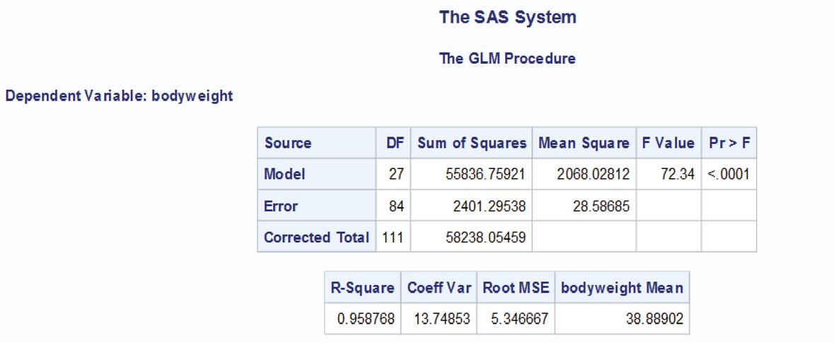
The data was analysed using the software SAS 9.3 (given in Appendix). The ANOVA table is given below

Source of Variation	DF	Sum of Squares	Mean Square	F Value	P Value
breed	7	5946.04	849.43	29.71	$<$0.001
Age group	6	5978.86	996.48	34.86	$<$0.001
feed	14	31717.14	2256.51	79.25	$<$0.001
Error	84	2401.29	28.59
Total	111	58238.05

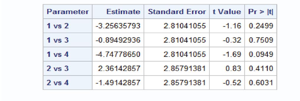
The breeds, age groups and feed effects are significant. The p value for estimating contrast pertaining to test vs control is also less than 0.05 so significant. The variance of contrast pertaining to test vs test and test vs control is given below

$$\mathrm{V}({\widehat{\tau }}_t-{\widehat{\tau }}_{t^{\prime }})=9.63,\mathit{t}\ne {\mathit{t}}^{\prime },$$

$$\mathit{t},{\mathit{t}}^{\prime }=1,2,\mathrm{\dots },{\mathit{v}}_1\mathit{t}\mathrm{and}{\mathit{t}}^{\prime }\mathrm{are}1\mathrm{st}\mathrm{associates}$$

$$\mathrm{V}({\widehat{\tau }}_t-{\widehat{\tau }}_{t^{\prime }})=9.78,\mathit{t}\ne {\mathit{t}}^{\prime },$$

$$\mathit{t},{\mathit{t}}^{\prime }=1,2,\mathrm{\dots },{\mathit{v}}_1\mathit{t}\mathrm{and}{\mathit{t}}^{\prime }\mathrm{are}2\mathrm{nd}\mathrm{associates}$$

$$\mathrm{V}({\widehat{\tau }}_t-{\widehat{\tau }}_{t^{\prime }})=9.63,\mathit{t}\ne {\mathit{t}}^{\prime },$$

$$\mathit{t},{\mathit{t}}^{\prime }=1,2,\mathrm{\dots },{\mathit{v}}_1\mathit{t}\mathrm{and}{\mathit{t}}^{\prime }\mathrm{are}3\mathrm{rd}\mathrm{associates}$$

$$\mathrm{V}({\widehat{\tau }}_t-{\widehat{\tau }}_{t^{\prime }})=8.58,\mathit{t}\ne {\mathit{t}}^{\prime },$$

$$\mathit{t},{\mathit{t}}^{\prime }=1,2,\mathrm{\dots },{\mathit{v}}_1,{\mathit{t}}^{\prime }=1\mathrm{test}\mathrm{treatments}\mathrm{with}\mathrm{control}$$

The contrasts pertaining to test vs. control are estimated with less variance (8.58). The average variance is 11.46.

Conclusion

The Generalized Row-Column (GRC) design is particularly useful when an experimenter faces limited resources but needs to evaluate a large number of treatments. To evaluate a group of test treatments against a pre-existing control treatment, the Partially Balanced Generalized Row-Column Design can be employed. This design is constructed using mutually orthogonal Latin squares (MOLS), resulting in a design that is partially balanced with respect to the test treatments. In this framework, there are four types of variances: three for the estimated contrasts among the test treatments, and one for the contrast between the test treatments and the control. The contrast between the test treatments and control is estimated with the least variance, which is of primary interest to the experimenter.

Acknowledgement

Authors are highly thankful to the learned reviewers for their valuable comments on the original version of the paper.

Appendix

SAS Code for Analysis

Data GRC;

Input breed agegroup feed bodyweight;

Cards;

1	1	2	21.00
2	1	9	57.09
…
8	7	13	65.39
;

PROC glm;

Class breed agegroup feed;

Model bodyweight = breed agegroup feed;

contrast ’control vs rest’ feed 1 1 1 1 1 1 1 1 1 1 1 1 1 1 -14;

estimate ’1 vs 2’ feed 1 -1 0 0 0 0 0 0 0 0 0 0 0 0 0;

estimate ’1 vs 3’ feed 1 0 -1 0 0 0 0 0 0 0 0 0 0 0 0;

estimate ’1 vs 4’ feed 1 0 0 -1 0 0 0 0 0 0 0 0 0 0 0;

estimate ’2 vs 3’ feed 0 1 -1 0 0 0 0 0 0 0 0 0 0 0 0;

estimate ’2 vs 4’ feed 0 1 0 -1 0 0 0 0 0 0 0 0 0 0 0;

Run;

The Analysis of Variance is given below:

$$\begin{array}{c}\mathrm{V}({\widehat{\tau }}_s-{\widehat{\tau }}_{{\mathit{s}}^{\prime }})=9.63,\mathit{s}\ne {\mathit{s}}^{\prime },\\ \mathit{s},{\mathit{s}}^{\prime }=1,2,\mathrm{\dots },{\mathit{v}}_1\mathit{s}\mathrm{and}{\mathit{s}}^{\prime }\mathrm{are}1\mathrm{st}\mathrm{associates}\\ \mathrm{V}({\widehat{\tau }}_s-{\widehat{\tau }}_{{\mathit{s}}^{\prime }})=9.78,\mathit{s}\ne {\mathit{s}}^{\prime },\\ \mathit{s},{\mathit{s}}^{\prime }=1,2,\mathrm{\dots },{\mathit{v}}_1\mathit{s}\mathrm{and}{\mathit{s}}^{\prime }\mathrm{are}2\mathrm{nd}\mathrm{associates}\\ \mathrm{V}({\widehat{\tau }}_s-{\widehat{\tau }}_{{\mathit{s}}^{\prime }})=9.63,\mathit{s}\ne {\mathit{s}}^{\prime },\\ \mathit{s},{\mathit{s}}^{\prime }=1,2,\mathrm{\dots },{\mathit{v}}_1\mathit{s}\mathrm{and}{\mathit{s}}^{\prime }\mathrm{are}3\mathrm{rd}\mathrm{associates}\\ \mathrm{V}({\widehat{\tau }}_s-{\widehat{\tau }}_{{\mathit{s}}^{\prime }})=8.58,\mathit{s}\ne {\mathit{s}}^{\prime },\\ \mathit{s}=1,2,\mathrm{\dots },{\mathit{v}}_1,{\mathit{s}}^{\prime }=1\mathrm{test}\mathrm{treatments}\mathrm{with}\mathrm{control}\end{array}$$

Average variance is 11.46.

References

Bailey, R. A. (1988). Semi Latin squares. Journal of Statistical Planning and Inference, 18, 299–312.

Bailey, R. A. (1992). Efficient semi-Latin squares. Statistica Sinica, 2, 413–437.

Bailey, R. A. and Monod, H. (2001). Efficient semi-Latin rectangles: Designs for plant disease experiments. Scandanavian Journal of Statistics, 28, 257–270.

Bedford, D. and Whitaker, R. M. (2001). A new construction for efficient semi-Latin squares. Journal of Statistical Planning and Inference, 98, 287–292.

Darby, L. A. and Gilbert, N. (1958). The Trojan Square. Euphytica, 7, 183–188.

Datta, A., Jaggi, S., Varghese, C. and Varghese, E. (2014). Structurally incomplete row-column designs with multiple units per cell. Statistics and Applications, 12 (1&2), 71–79.

Datta, A., Jaggi, S., Varghese, C. and Varghese, E. (2015). Some series of row-column designs with multiple units per cell. Calcutta Statistical Association Bulletin, 67(265–266), 89–99.

Datta, A., Jaggi, S., Varghese, C. and Varghese, E. (2016). Series of Incomplete Row-Column Designs with Two Units per Cell. Advances in Methodology and Statistics. 13(1), 17–25.

Datta, A., Jaggi, S., Varghese, E. and Varghese, C. (2017). Generalized Confounded Row- Column Designs. Communication in Statistics: Theory and Methods. 46(12), 6213–6221.

Edmondson, R. N. (1998). Trojan square and incomplete Trojan square design for crop research. Journal of Agricultural Science, 131, 135–142.

Harshbarger, B. and Davis, L. L. (1952). Latinized rectangular lattices. Biometrics, 8, 73–84.

Jaggi, S., Varghese, C., Varghese, E. and Sharma, V. K. (2010). Generalized incomplete Trojan-type designs. Statistics and Probability Letters, 80, 706–710.

Preece, D. A. and Freeman, G. H. (1983). Semi-Latin squares and related designs. Journal of Royal Statistical Society, B 45, 267–277.

Williams, E. R. (1986). Row and column designs with contiguous replicates. Australian Journal of Statistics, 28, 154–163.

Biographies

Anindita Datta is a Scientist in the Division of Design of Experiments at the ICAR-Indian Agricultural Statistics Research Institute, New Delhi. She handled 8 research projects including those funded by NAHEP. She has published around 50 research papers in international/national journals of high repute. She has received the ‘Jawaharlal Nehru Award for P.G. Outstanding Doctoral Thesis Research in Agricultural and Allied Sciences 2017 of ICAR and Dr. G.R. Seth Young Scientist memorial awards of Indian Society of Agricultural Statistics. She has been involved in teaching Agricultural Statistics for the last 9 years to M.Sc. and Ph. D. students of PG School, IARI, Delhi. She has organized many training programmes and workshops as coordinator/co-coordinator. Her research areas of interest are ‘Construction and analysis of designs for various experimental situations in agriculture’ and ‘Web generation and analysis of experimental designs’.

Seema Jaggi is currently serving as Assistant Director General (Human Resource Development) in the Agricultural Education Division of ICAR, a position she has held since April 2021. Her career at ICAR–IASRI includes serving as Scientist (1992–1997), Scientist (Senior Scale) (1997–2001), Senior (2001–2008), and Principal Scientist (2009 onwards). She also worked as Professor (Agricultural Statistics) from 2014 to 2021 and as Officiating Head, Division of Design of Experiments, from 2015 to 2021. She has received numerous awards, including the ICAR Panjabrao Deshmukh Outstanding Woman Scientist Award (2017), ICAR Bharat Ratna Dr. C. Subramaniam Award for Outstanding Teachers (2013), INSA Teacher Award (2015), ISAS Sankhyiki Bhushan Award (2022), and several others recognizing her contributions to teaching, research, and publication. Her major research areas include Agricultural Statistics, Design of Experiments, Statistical Computing, and Agricultural Education.

Cini Varghese is a Principal Scientist in the Division of Design of Experiments at the ICAR-Indian Agricultural Statistics Research Institute, New Delhi. She has handled 24 research projects including those funded by Department of Science and Technology, New Delhi, AP Cess fund as well as National fund of ICAR. She is Professor in the discipline of Agricultural Statistics and has been involved in teaching Agricultural Statistics for the last 27 years to M.Sc. and Ph. D. students of PG School, IARI, New Delhi. She has guided eight M.Sc. students and six Ph.D. students as Chairperson. She has organized many training programmes and workshops as coordinator/co-coordinator. Her research areas of interest are ‘Construction and analysis of designs for various experimental situations in agriculture’. She has published around 195 research papers in international/national journals of high repute and developed a number of software packages. She has received the ‘Lal Bahadur Shastri Young Scientist Award’ of ICAR for her outstanding contributions in the field of Social Sciences.

Eldho Varghese is a Senior Scientist in the Fishery Resources Assessment, Economics and Extension Division at ICAR–CMFRI, Kochi, a position he has held since 2022. He previously served as Scientist at ICAR–IASRI, New Delhi (2010–2017), and at ICAR–CMFRI, Kochi (2017–2019). He has received several honours, including the IARI Merit Medal (2012), Lal Bahadur Shastri Outstanding Young Scientist Award (2017), NAAS Young Scientist Award (2017–18), and NAAS Associateship (2023). He is Associate Editor of Model Assisted Statistics and Applications since 2012 and served as Honorary Joint Secretary of the Indian Society of Agricultural Statistics (2020–2023). He is an elected member of the International Statistical Institute and has represented India in expert committees and international meetings, including BOBP-IGO–FAO (2023) and the IOTC-FAO 20WPDCS (2024). His key research areas include Agricultural Statistics, Design of Experiments, Statistical Computing, Fish Stock Assessment, and Deep Learning Models.

Arpan Bhowmik is a Senior Scientist at ICAR-Indian Agricultural Research Institute, Gogamukh, Dhemaji, Assam. He previously served as Scientist at ICAR–IASRI, New Delhi (2012–2022). He has received several honours, including NAAS Associateship-2025, Best Scientist of the year-2024-25 at IARI Assam, IARI Merit Medal for Ph.D., International Travel Support for Young Scientist from SERB, DST, GOI for attending III LACSC at University of Costa Rica in 2018, Dr. G.R. Seth Memorial Young Scientist Award from Indian Society of Agricultural Statistics. He published more than 150 research papers in various national and international journals.

Mohd Harun is working as Scientist at ICAR-Indian Agricultural Statistics Research Institute for more than 9 years. His major expertise is in Design of Experiments. His area of research includes Block Designs, Row-Column Designs, Mating Designs, Screening Designs, space-filling designs, etc. He has Published more than 60 research papers; several popular articles, R-Packages, SAS macros. He is the recipient of GR Seth Memorial young scientist award, Dr R.K. Arora Best Paper Award, Nehru Memorial Gold Medal. He has organized many training programmes, workshop, etc.

Med Ram Verma is presently working as a Head, Division of Design of Experiments, ICAR-IASRI, Pusa, New Delhi since July 2023. He joined Agricultural Research Service in 2003. He joined ICAR-IVRI, Izatnagar Bareilly as a Senior Scientist in December 2009. He guided 4 Ph.D. and 10 M.V.Sc. students in the discipline of Biostatistics. He was awarded with “Best Teacher Award” by IVRI Deemed University in 2016. He was awarded with “Bharat Ratna Dr. C. Subramaniam Award for Outstanding Teachers” in 2019 by ICAR. He is the Fellow of Indian Society of Agricultural Statistics and Elected Member of International Statistical Institute, Netherlands. He is the Editorial Board Member and reviewer of the several journals. He published 260 research papers with total citations 2923 (h index 28 and i-10 Index 76).

Journal of Reliability and Statistical Studies, Vol. 19, Issue 1 (2026), 101–118
doi: 10.13052/jrss0974-8024.1915
© 2026 River Publishers