Stress and Strength Reliability Estimation for the Inverse Family of Distributions using Bayesian Analysis

Kuldeep Singh Chauhan^1,* and Sachin Tomer²

¹Department of Statistics, Ram Lal Anand College, University of Delhi, India
²Department of Statistics, Ramanujan College, University of Delhi, India
E-mail: kuldeepsinghchauhan.stat@rla.du.ac.in
*Corresponding Author

Received 28 July 2025; Accepted 06 March 2026

Abstract

A Bayesian model to study stress-strength reliability $P=P(Y<X)$, which makes use of parameters in the family of the inverse distributions. For the reliability function and for the stress-strength parameter, Bayes estimators are obtained under SELF and GELF. When this is appropriate, conjugate priors will be introduced into estimators, which will be constituted using different powers of the unknown parameters. Performance of these estimators is determined by a simulation-based methodology and large numbers of bootstrap replications. The findings show that, especially in small-sample circumstances, the Bayesian estimators based on SELF perform better than those based on GELF. The performance difference closes as the sample sizes grow. The exploration of this paper displays that the inverse family can be altered for several common distributions, which have more significant practical implications when analyzing reliability.

Keywords: Inverse family of distributions, stress-strength model, Bayesian estimation, squared error loss function, general entropy loss function, reliability function, bootstrap.

1 Introduction

The study of system reliability and stress-strength reliability under various types of stress is a major area of investigation in applied statistics and reliability engineering. Reliability can be measured by a function called the reliability function $R(t)$, where $t$ represents time. This means that if $X$ is the random variable representing the lifetime of some item, then $R(t)=P(X>t)$. A second reliability measurement that is commonly used to determine reliability in a stress-strength model is $P=P(Y<X)$. There have been a number of Bayesian studies done concerning the estimation of reliability since Bayesian analysis provides a method of incorporating past studies. Zahra et al. [23] provided evidence of the utility of Bayesian estimation using Pareto distributions. Studies using Bayesian estimation were carried out by Mahto [13] on inverted exponentiated distributions and by Kundu et al. [4] on Weibull distributions. Haijing et al. [25] also developed new methodologies to enhance multistate models, including objective Bayesian techniques. Shubham and Garg [19] and also Mahdi et al. [22] and by Abdulhakim et al. [20] used similar methodologies to evaluate non-Bayesian and Bayesian estimates of stress–strength reliability for Topp-Leone distribution and power-modified Lindley distributions sequentially. Traditional binary stress–strength reliability models have evolved into more complex models of dependence and conditions, as shown in the literature, described in the Marshall–Olkin Weibull distribution by Liming et al. [18]. In addition to general innovative applications of probability distributions to reliability studies, as seen in the inverse Chen distribution by Agiwal [15] and generalized inverted exponential distributions by Kumari [12], we have shown how many of the applications can be specific to particular applications. Further contributions to trade-offs in statistical contexts have been made through comparative analyses and interactive research on the trade-offs between Bayesian and frequentist approaches in various statistical problems by Sarah and Ali [17]. Therefore, all these applications contribute to our understanding of how the field has developed and the availability of the knowledge and tools to study and improve system reliability, and open the way for future discoveries about hybrid techniques and new distributions that will be useful.

The progress achieved, especially after adopting non-Bayesian and Bayesian approaches to estimation, is reflected in the models. However, the increasing complexity and sophistication of the systems, and the desire for accurate reliability estimates have motivated the development of special statistical distributions and more complex estimations.

The new contributions examined in this paper are Bayesian approaches, advanced models, and distribution-specific methods. From an examination of the developments reviewed above, we hope to present a global view of the evolution of research on stress-strength reliability in terms of significant practices and applications. Each of the papers reviewed is associated with various statistical distributions inverse, Pareto, Weibull, and Topp-Leone, etc.) and comments on the applicability of each distribution to real-world studies. Thus, a comprehensive review of the developments mentioned above, emphasizing both their theoretical and practical values are necessary.

2 Inverse Family of Distributions

Suppose that a random variable $X$ has p.d.f.

$$\begin{array}{c}\hfill f(x;\mu ,\nu ,\theta )=\frac{{\mu }^{\nu }{G}^{\nu -1}(x^{-1};\theta )G^{\prime }(x^{-1};\theta )}{x^{\nu }\mathrm{\Gamma }(\nu )}\exp \left(-\mu G(x^{-1};\theta )\right),\\ \hfill x>0,\mu ,\nu >0.\end{array}$$

(1)

Here, $G(x^{-1};\theta )$ depends on the parameter $\theta$ and is a function of $x$. $G^{\prime }(x^{-1};\theta )$ is the derivative of $G(x;\theta )$ with respect to $x^{-1}$. Equation (1) shows that the above distribution can be converted into the various distributions suggested by [16]. Chauhan and Sharma [24] used the suggested family of distributions to estimate a sequential testing procedure for the parameters of the inverse distribution family. As special examples, the distribution above can be transformed into the following distributions: If $G(x;\theta )=x^2,\nu =k+1(k\ge 0),\left(k=\frac{-1}{2}\right)$ provide the inverse half-normal distribution and $(\mathrm{k}=0)$ the inverse Rayleigh distribution. If $G(x;\theta )=\log \left(1+\frac{x^b}{{\delta }^b}\right),b>0,\delta >0,\nu =1$, provide the inverse log-logistic model. If $G(x;\theta )=\log \left(1+\frac{x^b}{{\delta }^b}\right),b>0,\delta =1,\nu >1$, provide the inverse Burr distribution. If $G(x;\theta )=\log \left(1+\frac{x^b}{{\delta }^b}\right),b=1,\delta >1,\nu >1$, provide the inverse Lomax distribution. If $G(x;\theta )=\frac{x^2}{2},\nu =\frac{h}{2}(h>0)$, it becomes the inverse Chi-square distribution. If $G(x;\theta )=\log \left(\frac{x}{a}\right)$ and $\nu =1$, obtain the inverse Pareto distribution. If $G(x;\theta )=x^r\exp (ax),r>0,a>0,\nu =1$, obtain the modified inverse Weibull distribution. If $G(x;\theta )=\mu x+\frac{\gamma x^2}{2},\gamma =1,\nu =1$, obtain the inverse linear exponential distribution. If $G(x;\theta )=\log x$, obtain the inverse of the log-gamma distribution. If $G(x;\theta )=x^p,p>0,\nu >0$, one obtains the inverse generalized gamma distribution.

For model (1), the reliability function at a specified time t

$$R(t)=P(X>t)=\exp \left(-\mu G(x^{-1};\theta )\right).$$

And $P=P(Y<X)$ represents the reliability of an item of random strength $X$ subject to random stress $Y$. We aim to estimate the reliability function $R(t)=P(X>t)$ and $P=P(Y<X)$ under Squared Error Loss Function (SELF) and General Entropy Loss Function (GELF).

3 Notations and Definitions

Suppose $n$ items are put on a test and the test is terminated after the first $r$ ordered observations are recorded. Let $0\le X_{(1)}\le \mathrm{\cdots }\le X_{(r)},0<r<n$ be the lifetimes of the first $r$ ordered observations. Obviously, ( $n-r$ ) items survived until $X_{(r)}$. Representing by $\underset{¯}{x}=(x_1,x_2,\mathrm{\dots }{x}_r),S={\sum }_{i=1}^{r}G(x_{(i)}^{-1};\theta )+(n-r)G(x_{(r)}^{-1};\theta )$ And the likelihood function

$$L(\mu \mid \underset{¯}{x})\propto {\mu }^{\nu n}\exp \left[-\mu \left(\sum _{i=1}^r\mathrm{G}(x_i^{-1};\theta )+(n-r)G(x_{(r)}^{-1};\theta )\right)\right]$$

We think through the natural conjugate prior model for $\alpha$, designating a gamma model

$$\pi (\mu )=\frac{b^d}{\mathrm{\Gamma }(d)}{\mu }^{d-1}\exp (-\mu b);b,d>0$$

Combining the above two equations, the posterior distribution of $\alpha$ by Bayes’ theorem,

$$h(\mu \mid S)=\frac{{(b+S)}^{n\beta +d}}{\mathrm{\Gamma }(n\beta +d)}{\mu }^{n\nu +d-1}\exp [-\mu (b+S)]$$

Let $X$ and $Y$ are two independent random variables with the PDF $f_1(x;{\mu }_1,{\nu }_1,{\theta }_1)$ and $f_2(y;{\mu }_2,{\nu }_2,{\theta }_2)$ sequentially.

Assume in a test that $n$ products are in $X$ and $m$ products are in $Y$ to estimate $R(t)$. And $S={\sum }_{i=1}^{r}G(x_{(i)}^{-1};{\theta }_1)+(n-r)G(x_{(r)}^{-1};{\theta }_1)$ and $T={\sum }_{i=1}^{r}H(y_{(i)}^{-1};{\theta }_2)+(m-u)G(y_{(u)}^{-1};{\theta }_2)$ . When ${\mu }_1$ and ${\mu }_2$ are unrecognized but ${\nu }_1,{\nu }_2,{\theta }_1,{\theta }_2$ are recognized. We research the conjugate priors for ${\mu }_1$ and ${\mu }_2$ are $(b_1,d_1)$ and $(b_2,d_2)$ correspondingly. The PDF of $S$ using Lemma 1 from Chaturvedi and Chauhan [8].

$$h(s;\mu )=\frac{{\mu }^{n\nu }}{\mathrm{\Gamma }(n\nu )}{s}^{n\nu -1}exp(-\mu s);\mu >0,\nu >0,n>0;0<s<\mathrm{\infty }$$

(2)

Signifying via ${\widehat{\delta }}_{BL}$, Bayes estimator of $\delta =\psi (\mu )$ with loss $L$ for assessing $\delta$ by $L\left({\widehat{\delta }}_B=\delta \right)$ correspondingly, the risk is explained through

$$R_L\left({\widehat{\delta }}_{BL}\right)=E_{(S\mid \mu )}\left\{L({\widehat{\delta }}_{BL},\delta )\right\}.$$

The posterior risk assessment used to evaluate $\delta$ by ${\widehat{\delta }}_{BL}$ is

$$R_{PL}\left({\widehat{\delta }}_{BL}\right)=E_{(\mu \mid S)}\left\{L({\widehat{\delta }}_{BL},\delta )\right\}$$

The Bayes risk assessment is used to evaluate $\delta$ by ${\widehat{\delta }}_{BL}$ is

$$R_{BL}\left({\widehat{\delta }}_{BL}\right)=E_S\left[E_{(\mu \mid S)}\left\{L({\widehat{\delta }}_{BL},\delta )\right\}\right]$$

We note that the posterior risk is self-establishing from $\mu$, the Bayes risk only takes the prior parameter, and the sample has no bearing on the risk of the Bayes estimator of $\delta$. Additionally, we note that the relationships that result

$$R_{BL}\left({\widehat{\delta }}_{BL}\right)=E_{\mu }\left\{R_L\left({\widehat{\delta }}_{BL}\right)\right\}.$$

And

$$R_{BL}\left({\widehat{\delta }}_{BL}\right)=E_S\left\{R_p\left({\widehat{\delta }}_{B^L}\right)\right\}$$

4 The Bayes Estimators of Reliability Using SELF

If p is a positive integer, the Bayes estimators of ${\mu }^{-p}$ and ${\mu }^p$ with SELF are specified through ${\widehat{\mu }}_{BS}^p$ and ${\widehat{\mu }}_{BS}^{-p}$ correspondingly,

${\widehat{\mu }}_{BS}^p$	$={\displaystyle \frac{\mathrm{\Gamma }(n\nu +d+p)}{\mathrm{\Gamma }(n\nu +d)}}{\left(b{\widehat{\mu }}_{BS}^p+S\right)}^{-p}$	(3)
${\widehat{\mu }}_{BS}^{-p}$	$={\displaystyle \frac{\mathrm{\Gamma }(n\nu +d-p)}{\mathrm{\Gamma }(n\nu +d)}}{\left(b\cdot {\widehat{\mu }}_{BS}^{-p}+S\right)}^p,\text{w}here,p<n\nu +d.$	(4)

The posterior mean for any function of $\mu$ under SELF is the Bayes estimator, according to (2).

Theorem 1: Bayes estimators of posterior risk and Bayes risk for powers of $\mu$ with SELF.

$R_S\left({\widehat{\mu }}_{BS}^p\right)$	$={\left({\displaystyle \frac{\mathrm{\Gamma }(n\nu +d+p)}{\mathrm{\Gamma }(n\nu +d)}}\right)}^2{b}^{2n\nu -2p}U(n\nu ,n\nu +1-2p,\mu b)+{\mu }^{2p}$
	$-2{\mu }^{p+n\nu }{b}^{n\nu -p}{\displaystyle \frac{\mathrm{\Gamma }(n\nu +d+p)}{\mathrm{\Gamma }(n\nu +d)}}U(n\nu ,n\nu +1-p,\mu b)$	(5)
$R_{PS}\left({\widehat{\mu }}_{BS}^p\right)$	$=\left[{\displaystyle \frac{\mathrm{\Gamma }(n\nu +d+2p)}{\mathrm{\Gamma }(n\nu +d)}}-{\left({\displaystyle \frac{\mathrm{\Gamma }(n\nu +d+p)}{\mathrm{\Gamma }(n\nu +d)}}\right)}^2\right]{(b+S)}^{-2p}$	(6)
$R_{BS}\left({\widehat{\mu }}_{BS}^p\right)$	$=\left[1-{\displaystyle \frac{\mathrm{\Gamma }{(n\nu +d+p)}^2}{\mathrm{\Gamma }(n\nu +d)\mathrm{\Gamma }(n\nu +d+2p)}}\right]b^{-2p}{\displaystyle \frac{\mathrm{\Gamma }(d+2p)}{\mathrm{\Gamma }(d)}}.$	(7)
$R_S\left({\widehat{\mu }}_{BS}^{-p}\right)$	$={\mu }^{-2p}+b^{n\nu +2p}{\mu }^{n\nu }$
	$\times [{\left({\displaystyle \frac{\mathrm{\Gamma }(n\nu +d-p)}{\mathrm{\Gamma }(n\nu +d)}}\right)}^{2}U(n\nu ,n\nu +2p+1,\mu b)$
	$-2{\mu }^{-p}\left({\displaystyle \frac{\mathrm{\Gamma }(n\nu +d-p)}{\mathrm{\Gamma }(n\nu +d)}}\right)b^{-p}U(n\nu ,n\nu +p+1,\mu b)]$	(8)
$R_{PS}\left({\widehat{\mu }}_{BS}^{-p}\right)$	$=\left[{\displaystyle \frac{\mathrm{\Gamma }(n\nu +d-2p)}{\mathrm{\Gamma }(n\nu +d)}}-{\left({\displaystyle \frac{\mathrm{\Gamma }(n\nu +d-p)}{\mathrm{\Gamma }(n\nu +d)}}\right)}^2\right]{(b+S)}^{2p};$
	$(2p<n\nu +d)$	(9)
$R_{BS}\left({\widehat{\mu }}_{BS}^{-p}\right)$	$=\left[1-{\displaystyle \frac{\mathrm{\Gamma }{(n\nu +d-p)}^2}{\mathrm{\Gamma }(n\nu +d)\mathrm{\Gamma }(n\nu +d-2p)}}\right]b^{2p}{\displaystyle \frac{\mathrm{\Gamma }(d-2p)}{\mathrm{\Gamma }(d)}}$	(10)

Proof: From (3), the risk for $({\widehat{\mu }}_{BS}^p)$ is

$R_S\left({\widehat{\mu }}_{BS}^p\right)$	$={\left({\displaystyle \frac{\mathrm{\Gamma }(n\nu +d+p)}{\mathrm{\Gamma }(n\nu +d)}}\right)}^2{E}_{(S\mid \mu )}{(b+S)}^{-2p}+{\mu }^{2p}$
	$-2{\mu }^p{\displaystyle \frac{\mathrm{\Gamma }(n\nu +d+p)}{\mathrm{\Gamma }(n\nu +d)}}{E}_{(S\mid \mu )}{(b+S)}^{-p}$	(11)

According to (2), if $q$ is a positive number,

$$E_{(S\mid \mu )}{(b+S)}^{-q}=\frac{{\mu }^{n\nu }}{b^q\mathrm{\Gamma }(n\nu )}{\int }_0^{\mathrm{\infty }}\frac{s^{n\nu -1}}{{(1+s/b)}^q}exp(-\mu s)\mathit{d}s.$$

(12)

From (11) and (12)

$R_S\left({\widehat{\mu }}_{BS}^p\right)$	$={\left({\displaystyle \frac{\mathrm{\Gamma }(n\nu +d+p)}{\mathrm{\Gamma }(n\nu +d)}}\right)}^2{\displaystyle \frac{{}_{b^{n\nu }}}{b^{2p}\mathrm{\Gamma }(n\nu )}}{\displaystyle {\int }_0^{\mathrm{\infty }}}{\displaystyle \frac{s^{n\nu -1}}{{(1+s/b)}^{2p}}}exp(-\mu s)\mathit{d}s$
	$+{\mu }^{2p}-2{\mu }^p{\displaystyle \frac{\mathrm{\Gamma }(n\nu +d+p)}{\mathrm{\Gamma }(n\nu +d)}}{\displaystyle \frac{{\mu }^{n\nu }}{b^p\mathrm{\Gamma }(n\nu )}}$
	$\times {\displaystyle {\int }_0^{\mathrm{\infty }}}{\displaystyle \frac{s^{n\nu -1}}{{(1+s/b)}^p}}exp(-\mu s)ds$	(13)

And we can achieve the result (5).

$R_{BS}\left({\widehat{\mu }}_{BS}^p\right)$	$=\left[{\displaystyle \frac{\mathrm{\Gamma }(n\nu +d+2p)}{\mathrm{\Gamma }(n\nu +d)}}-{\left({\displaystyle \frac{\mathrm{\Gamma }(n\nu +d+p)}{\mathrm{\Gamma }(n\nu +d)}}\right)}^2\right]{\displaystyle \frac{b^d}{B(n\nu ,d)}}$
	$\times {\displaystyle {\int }_0^{\mathrm{\infty }}}{\displaystyle \frac{s^{n\nu -1}}{{(s+b)}^{n\nu +d+2p}}}ds$

And we can achieve the result (7)

$$R_S\left({\widehat{\mu }}_{BS}^{-p}\right)=E_{(S\mid \mu )}{\left({\widehat{\mu }}_{BS}^{-p}\right)}^2-2{\mu }^{-p}{E}_{(S\mid \mu )}\left({\widehat{\mu }}_{BS}^{-p}\right)+{\mu }^{-2p}.$$

(14)

Using (2), $q$ is a positive number.

$$E_{(S\mid \mu )}{(b+S)}^q={\int }_0^{\mathrm{\infty }}\frac{{\mu }^{n\nu }}{\mathrm{\Gamma }(n\nu )}{s}^{n\nu -1}exp(-\mu s){(b+s)}^q\mathit{d}s.$$

(15)

From (14) and (15) can be attained

$R_S\left({\widehat{\mu }}_{BS}^{-p}\right)$	$={\left({\displaystyle \frac{\mathrm{\Gamma }(n\nu +d-p)}{\mathrm{\Gamma }(n\nu +d)}}\right)}^2{\displaystyle \frac{{\mu }^{n\nu }}{\mathrm{\Gamma }(n\nu )}}{b}^{2p}{\displaystyle {\int }_0^{\mathrm{\infty }}}{\displaystyle \frac{s^{n\nu -1}{e}^{-\mu s}}{{(1+s/b)}^{-2p}}}\mathit{d}s+{\mu }^{-2p}$
	$-2{\mu }^{-p}\left({\displaystyle \frac{\mathrm{\Gamma }(n\nu +d-p)}{\mathrm{\Gamma }(n\nu +d)}}\right){\displaystyle \frac{{\mu }^{n\nu }}{\mathrm{\Gamma }(n\nu )}}{b}^p{\displaystyle {\int }_0^{\mathrm{\infty }}}{\displaystyle \frac{s^{n\nu -1}{e}^{-\mu s}}{{(1+s/b)}^{-p}}}\mathit{d}s$	(16)

And we can achieve the result (8).

The integrals (4) and (4) are evaluated using the identity,

$U(a,b,z)={\displaystyle \frac{1}{\mathrm{\Gamma }(a)}}{\displaystyle {\int }_0^{\mathrm{\infty }}}{e}^{-zt}{t}^{a-1}{(1+t)}^{b-a-1}\mathit{d}t,\text{for}a>0,z>0$

where $U(a,b,z)$ is the Tricomi confluent hypergeometric function [1].

Consequently, we can achieve (6), (9) and (10).

Lemma 1: The distribution $(1)$ of the Bayes estimator with SELF for $f(x;\mu ,\nu ,\theta )$ is

$${\widehat{f}}_{BS}(x;\mu ,\nu ,\theta )=\frac{G^{\nu -1}(x^{-1};\theta )G^{{}^{\prime }}(x^{-1};\theta )}{x^2{(S+b)}^{\nu }B(n\nu +d,\nu )}{\left[1+\frac{G(x^{-1};\theta )}{S+b}\right]}^{-(n\nu +d+\nu )}$$

(17)

Proof: Compose (1) as

$$f(x;\mu ,\nu ,\theta )=\frac{G^{\nu -1}(x^{-1};\theta )G^{{}^{\prime }}(x^{-1};\theta )}{x^2\mathrm{\Gamma }(\nu )}\sum _{i=0}^{\mathrm{\infty }}{(-1)}^i\frac{G^i(x^{-1};\theta )}{i!}{\mu }^{i+\nu }$$

(18)

From (4), and using Lemma 1 of Chaturvedi and Tomer [7] and (5),

${\widehat{f}}_{BS}(x;\mu ,\nu ,\underset{¯}{\theta })$	$={\displaystyle \frac{G^{\nu -1}(x^{-1};\theta )G^{{}^{\prime }}(x^{-1};\theta )}{x^2\mathrm{\Gamma }(\nu )}}{\displaystyle \sum _{i=0}^{\mathrm{\infty }}}{(-1)}^i{\displaystyle \frac{G^i(x^{-1};\theta )}{i!}}{\widehat{\mu }}_{BS}^{i+\nu }$	(19)
	$={\displaystyle \frac{G^{\nu -1}(x^{-1};\theta )G^{{}^{\prime }}(x^{-1};\theta )}{x^2\mathrm{\Gamma }(\nu )}}{\displaystyle \sum _{i=0}^{\mathrm{\infty }}}{(-1)}^i$
	$\times {\displaystyle \frac{{\left[G(x^{-1};\theta )\right]}^i\mathrm{\Gamma }(n\nu +d+i+\nu )}{i!\mathrm{\Gamma }(n\nu +d)}}{(S+b)}^{-(i+\nu )}$
	$={\displaystyle \frac{G^{\nu -1}(x^{-1};\theta )G^{{}^{\prime }}(x^{-1};\theta )}{x^2{(S+b)}^{\nu }B(n\nu +d,\nu )}}{\displaystyle \sum _{i=0}^{\mathrm{\infty }}}{(-1)}^i$
	$\times {\left[{\displaystyle \frac{G(x^{-1};\theta )}{S+b}}\right]}^i\left(\begin{array}{c}n\nu +d+i+\nu -1\\ i\end{array}\right)$	(21)

and the lemma holds.

Theorem 2: The reliability function of the Bayes estimator through SELF

${\widehat{R}}_{BS}(t)$	$={\displaystyle {\int }_t^{\mathrm{\infty }}}{\displaystyle \frac{G^{\nu -1}(x^{-1};\theta )G^{{}^{\prime }}(x^{-1};\theta )}{x^2{(S+b)}^{\nu }B(n\nu +d,\nu )}}$
	$\times {\left[1+{\displaystyle \frac{G(x^{-1};\theta )}{S+b}}\right]}^{-(n\nu +d+\nu )}dx.$	(22)

Proof: We get

${\displaystyle {\int }_t^{\mathrm{\infty }}}{\widehat{f}}_{BS}(x;a,\mu ,\nu ,\underset{¯}{\theta })$	$={\displaystyle {\int }_t^{\mathrm{\infty }}}{E}_{(\mu \mid S)}(f(x;a,\mu ,\nu ,\underset{¯}{\theta }))\mathit{d}x$
	$=E_{(\mu \mid S)}[R(t)]=\widehat{R}{(t)}_{BS}$	(23)

The result is derived from Equation (18) and Lemma 1.

Corollary 1: While$\nu =1$,

$${\widehat{R}}_{BS}(t)={\int }_t^{\mathrm{\infty }}\frac{G^{{}^{\prime }}(x^{-1};\theta )}{x^2(S+b)B(n+d,1)}{\left[1+\frac{G(x^{-1};\theta )}{S+b}\right]}^{-(n+d+1)}\mathit{d}x.$$

For '$P$ ', we use SELF to obtain the Bayes estimator.

Theorem 3:

${\widehat{P}}_{BS}$	$={\displaystyle \frac{1}{(T+b_2){\nu }_{2B(}m{\nu }_2+d_2,{\nu }_2)}}{\displaystyle \frac{1}{\left(S+b_1\right){\nu }_{1}B(n{\nu }_1+d_1,{\nu }_1)}}$
	$\times {\displaystyle {\int }_0^{\mathrm{\infty }}}{\displaystyle \frac{H^{{\nu }_2-1}(y^{-1};{\theta }_2)H^{{}^{\prime }}(y^{-1};{\theta }_2)}{y^2}}$
	$\times {\left[1+{\displaystyle \frac{H(y^{-1};{\theta }_2)}{T+b_2}}\right]}^{-\left(m{\nu }_2+d_2+{\nu }_2\right)}$
	$\times {\displaystyle {\int }_y^{\mathrm{\infty }}}{\displaystyle \frac{G^{{\nu }_1-1}(x^{-1};{\theta }_1)G^{{}^{\prime }}(x^{-1};{\theta }_1)}{x^2}}$
	$\times {\left[1+{\displaystyle \frac{G(x^{-1};{\theta }_1)}{s+b_1}}\right]}^{-\left(n{\nu }_1+d_1+{\nu }_1\right)}dxdy.$	(24)

Proof:

${\widehat{P}}_{BS}$	$={\displaystyle {\int }_{y=0}^{\mathrm{\infty }}}{\displaystyle {\int }_{x=y}^{\mathrm{\infty }}}{\widehat{f}}_{1BS}(x;{\mu }_1,{\nu }_1,{\theta }_1){\widehat{f}}_{2BS}(y;{\mu }_2,{\nu }_2,{\theta }_2)\mathit{d}x\mathit{d}y$
	$={\displaystyle {\int }_{y=0}^{\mathrm{\infty }}}{\widehat{f}}_{2BS}(y;{\mu }_2,{\nu }_2,{\theta }_2){\widehat{R}}_{BS}(y;{\mu }_1,{\nu }_1,{\theta }_1)\mathit{d}y$	(25)

Equation (4) and Lemma 1 are used to obtain the result.

Remark 1: To derive Bayes estimators of the stress-strength setup and reliability function, the researcher primarily used the terms of parameters and their Bayes estimators, i.e., posterior mean through SELF, in the collected works. The offered method includes the stress-strength setup, Bayes estimators, and the reliability function. The Bayes estimator is available, the other does not require its terms.

5 The Bayes Estimators of Reliability Using GELF

Suppose $\widehat{\mu }$ be the estimator of $\mu$, formerly GELF

$$L(\widehat{\mu },\mu )={\left(\frac{\widehat{\mu }}{\mu }\right)}^k-k\ln \left(\frac{\widehat{\mu }}{\mu }\right)-1$$

Where $k\ne 0$ is a constant.

$\widehat{\mu }$ with GELF, Using Calabria and Pulcini [2]

$${\widehat{\mu }}_{BG}={\left[E_{(\mu \mid S)}\left\{{\mu }^{-k}\right\}\right]}^{-1/k}$$

(26)

Theorem 4: Bayes estimators of ${\mu }^p$ and${\mu }^{-p}$, using GELF for a positive number p by ${\widehat{\mu }}_{BG}^p$ and ${\widehat{\mu }}_{BG}^{-p}$ are provided in order,

$${\widehat{\mu }}_{BG}^p=\left(\frac{\mathrm{\Gamma }(n\nu +d)}{\mathrm{\Gamma }\left(n\nu +d-p\right)}\right){(b+S)}^{-p}$$

(27)

and

$${\widehat{\mu }}_{BG}^{-p}=\left(\frac{\mathrm{\Gamma }(n\nu +d)}{\mathrm{\Gamma }\left(n\nu +d+p\right)}\right){(b+S)}^p.\text{where}n\nu +d>p$$

(28)

Proof: Achieved from (26) and Theorem 1.

Theorem 5: The terms posterior risks, Bayes risks with GELF, and the Bayes estimators of powers of $\mu$ should be developed using GELF.

$R_G\left({\widehat{\mu }}_{BG}^p\right)$	$=\left({\displaystyle \frac{\mathrm{\Gamma }(n\nu +d)}{\mathrm{\Gamma }(n\nu +d-p)}}\right){\mu }^{n\nu -p}{b}^{n\nu -p}U(n\nu ,n\nu -p+1,\mu b)$
	$+\ln \left({\displaystyle \frac{{\mu }^p\mathrm{\Gamma }(n\nu +d-p)}{\mathrm{\Gamma }(n\nu +d)}}\right)-1$
	$+p\left[\psi (n\nu )-\ln \mu +b^{n\nu }{\mu }^{n\nu }U(n\nu ,n\nu +1,\mu b)\ln (\mu b)\right]$	(29)
$R_{PG}\left({\widehat{\mu }}_{BG}^p\right)$	$=p[\psi (n\nu +d)]-ln\left({\displaystyle \frac{\mathrm{\Gamma }(n\nu +d)}{\mathrm{\Gamma }\left(n\nu +d-p\right)}}\right)$	(30)
$R_{BG}\left({\widehat{\mu }}_{BG}^p\right)$	$=p[\psi (n\nu +d)]-ln\left({\displaystyle \frac{\mathrm{\Gamma }(n\nu +d)}{\mathrm{\Gamma }\left(n\nu +d-p\right)}}\right)$	(31)
$R_G\left({\widehat{\mu }}_{BG}^{-p}\right)$	$=\left({\displaystyle \frac{\mathrm{\Gamma }(n\nu +d)}{\mathrm{\Gamma }(n\nu +d+p)}}\right){(\mu b)}^{p+n\nu }U(n\nu ,n\nu -p,\mu b)$	(32)
$R_{PG}\left({\widehat{\mu }}_{BG}^{-p}\right)$	$=-ln\left({\displaystyle \frac{\mathrm{\Gamma }(n\nu +d)}{\mathrm{\Gamma }\left(n\nu +d+p\right)}}\right)-p[\psi (n\nu +d)]$	(33)
$R_{BG}\left({\widehat{\mu }}_{BG}^{-p}\right)$	$=-ln\left({\displaystyle \frac{\mathrm{\Gamma }(n\nu +d)}{\mathrm{\Gamma }\left(n\nu +d+p\right)}}\right)-p[\psi (n\nu +d)]$	(34)

where

$$\psi (x)=\frac{d}{dx}log\mathrm{\Gamma }(x)$$

Proof: From (27)

$R_G\left({\widehat{\mu }}_{BG}^p\right)$	$=E_{(S\mid \mu )}\left[\left\{\left({\displaystyle \frac{\mathrm{\Gamma }(n\nu +d)}{\mathrm{\Gamma }\left(n\nu +d-p\right)}}\right){\displaystyle \frac{{(b+S)}^{-p}}{{\mu }^p}}\right\}\right]$
	$-ln\left[\left({\displaystyle \frac{\mathrm{\Gamma }(n\nu +d)}{\mathrm{\Gamma }\left(n\nu +d-p\right)}}\right){\displaystyle \frac{{(b+S)}^{-p}}{{\mu }^p}}\right]-1$	(35)

(5) achieved by (2) and (5).

$R_G\left({\widehat{\mu }}_{BG}^p\right)$	$=\left({\displaystyle \frac{\mathrm{\Gamma }(n\nu +d)}{\mathrm{\Gamma }\left(n\nu +d-p\right)}}\right){\left({\displaystyle \frac{1}{\mu }}\right)}^p$
	$\times {\displaystyle {\int }_0^{\mathrm{\infty }}}{(b+s)}^{-p}{\displaystyle \frac{{\mu }^{n\nu }}{\mathrm{\Gamma }(n\nu )}}{s}^{n\nu -1}exp(-\mu s)ds$
	$-ln\left({\displaystyle \frac{\mathrm{\Gamma }(n\nu +d)}{\mathrm{\Gamma }\left(n\nu +d-p\right)}}\right)$
	$+{\displaystyle \frac{p{\mu }^{n\nu }}{\mathrm{\Gamma }(n\nu )}}{\displaystyle {\int }_0^{\mathrm{\infty }}}{s}^{(n\nu -1)}exp(-\mu s)ln[(b+s)\mu ]\mathit{d}s-1$	(36)

And (29) achieved.

Using (28), the posterior risk of ${\widehat{\mu }}_{BG}^p$ with GELF

$R_{PG}\left({\widehat{\mu }}_{BG}^p\right)$	$=E_{(\mu \mid S)}[\left({\displaystyle \frac{\mathrm{\Gamma }(n\nu +d)}{\mathrm{\Gamma }\left(n\nu +d-p\right)}}\right){\left({\displaystyle \frac{1}{(b+S)}}\right)}^p{E}_{(\mu \mid S)}\left({\mu }^{-p}\right)$
	$-ln{\displaystyle \frac{\mathrm{\Gamma }(n\nu +d)}{\mathrm{\Gamma }\left(n\nu +d-p\right)}}+E_{(\mu \mid S)}ln\{\mu (b+S)\}-1]$	(37)

(38) achieved by (2) and (5)

$$R_G\left({\widehat{\mu }}_{BG}^{-p}\right)=\left(\frac{\mathrm{\Gamma }(n\nu +d)}{\mathrm{\Gamma }(n\nu +d+p)}\right){\mu }^{p+n\nu }{\int }_0^{\mathrm{\infty }}{(b+s)}^p{s}^{n\nu -1}\exp (-\mu s)\mathit{d}s$$

(38)

The integrals (5) and (38) are evaluated using the identity,

$U(a,b,z)={\displaystyle \frac{1}{\mathrm{\Gamma }(a)}}{\displaystyle {\int }_0^{\mathrm{\infty }}}{e}^{-zt}{t}^{a-1}{(1+t)}^{b-a-1}\mathit{d}t,\text{for}a>0,z>0$

where $U(a,b,z)$ is the Tricomi confluent hypergeometric function [1].

And using the findings of Ryzhik and Gradshteyn [5] that

$${\int }_0^{\mathrm{\infty }}{x}^{\alpha -1}{e}^{-\beta x}\ln xdx=\frac{\mathrm{\Gamma }(\alpha )}{{\beta }^{\alpha }}[\mathrm{\Psi }(\alpha )-\ln \beta ]$$

(39)

Using (5) and (5), results (30) were obtained. Equation (30) therefore shows that $R_{PG}\left({\widehat{\mu }}_{BG}^p\right)$ is independent of S. Its posterior risk is similar to the Bayes risk of ${\widehat{\mu }}_{BG}^p$. Sequentially, the results (32), (33), and (34) are comparable to those of (29), (30), and (31).

Remark 2: It is interesting to observe that the phrases for $R_{BG}\left({\widehat{\mu }}_{BG}^p\right),R_{PG}\left({\widehat{\mu }}_{BG}^p\right),R_{PG}\left({\widehat{\mu }}_{BG}^{-p}\right),R_{PG}\left({\widehat{\mu }}_{BG}^{-p}\right)$ are identical.

Theorem 6: Under GELF, Bayes estimator for $R(t)$

${\widehat{R}}_{BG}(t)$	$=[{\displaystyle {\int }_0^{\mathrm{\infty }}}{\displaystyle \frac{{(b+S)}^{n\nu +d}}{\mathrm{\Gamma }(n\nu +d)}}{\mu }^{n\nu +d-1}{e}^{-\mu (b+S)}$	(40)
	$\times {\left\{{\displaystyle {\int }_0^{\mu }}G(t^{-1};\theta ){\displaystyle \frac{e^{-z}{z}^{\nu -1}}{\mathrm{\Gamma }\nu }}dz\right\}}^{-1}d\mu ]{}^{-1}$

Proof: The result obtained by using (2) and (26).

Theorem 7: The Bayes estimator of P under GELF

${\widehat{P}}_{BG}$	$=[{\displaystyle \frac{{(b_1+S)}^{n+d_1}{(b_2+T)}^{m+d_2}}{B(n+d_1,m+d_2)}}$	(41)
	$\times {\displaystyle {\int }_0^1}{\displaystyle \frac{P^{n+d_1-1}{(1-P)}^{m+d_2-1}}{{\left[P(b_1+S)+(1-P)(b_2+T)\right]}^{n+m+d_1+d_2}}}dP]{}^{-1}$

Proof: If

$P$	$={\displaystyle {\int }_{y=0}^{\mathrm{\infty }}}{\displaystyle {\int }_{x=y}^{\mathrm{\infty }}}{\displaystyle \frac{{\mu }_1{\mu }_2}{x^2{y}^2}}{G}^{\prime }(x^{-1};\theta )G^{\prime }(y^{-1};\theta )\mathit{d}x\mathit{d}y$
${\theta }_1$	$={\theta }_2=\theta ,h^{-1}(T)=g^{-1}(S),{\nu }_1={\nu }_2=1$
$P$	$={\displaystyle {\int }_{y=0}^{a_2^{-1}}}{\displaystyle {\int }_{x=y}^{\mathrm{\infty }}}{\displaystyle \frac{{\mu }_1{\mu }_2}{x^2{y}^2}}{G}^{\prime }(x^{-1};\theta )G^{\prime }(y^{-1};\theta )$
	$\times \exp \left[-{\mu }_{1}G(x^{-1};\theta )\right]\exp \left[-{\mu }_{2}G(y^{-1};\theta )\right]dxdy$
$P$	$={\displaystyle {\int }_{y=0}^{\mathrm{\infty }}}{\displaystyle \frac{{\mu }_2{G}^{\prime }(y^{-1};\theta )\exp \left[-{\mu }_{2}G(y^{-1};\theta )\right]}{y^2}}$
	$\times {\displaystyle {\int }_0^{{\mu }_1}}G(y^{-1};\theta )\exp (-z)dzdy$
$P$	$={\displaystyle \frac{{\mu }_1}{{\mu }_1+{\mu }_2}}$

Using (2), the posterior likelihood pdf of ${\mu }_1$ and ${\mu }_2$ is

$h({\mu }_1,{\mu }_2)$	$={\displaystyle \frac{{\left(b_1+S\right)}^{n+d_1}{\left(b_2+T\right)}^{m+d_2}}{\mathrm{\Gamma }\left(n+d_1\right)\mathrm{\Gamma }\left(m+d_2\right)}}{\mu }_1^{n+d_1-1}{\mu }_2^{m+d_2-1}$
	$exp\left(-{\mu }_1\left(b_1+S\right)\right)exp\left(-{\mu }_2\left(b_2+T\right)\right)$	(42)

Suppose the renovations of $P=\frac{{\mu }_1}{{\mu }_1+{\mu }_2}$ and $w={\mu }_1+{\mu }_2$, so as to ${\mu }_1=wP$ also ${\mu }_2=w(1-P).$ The alteration for Jacobean is $w$. As of (40), together with w, the posterior likelihood pdf of P,

$h(P,w)$	$={\displaystyle \frac{{\left(b_1+S\right)}^{n+d_1{\left(b_2+T\right)}^{m+d_2}}}{\mathrm{\Gamma }\left(n+d_1\right)\mathrm{\Gamma }\left(m+d_2\right)}}{P}^{n+d_1-1}{(1-P)}^{m+d_2-1}{w}^{n+m+d_1+d_2-1}$
	$exp\left(-w\left(b_1+S\right)P+(1-P)\left(b_2+T\right)\right);$
	$0<w<\mathrm{\infty },0<P<1$	(43)

Equation (5) is integrated for $w$, and the posterior density function of P is obtained.

$h(P)$	$={\displaystyle \frac{{\left(b_1+S\right)}^{n+d_1}{\left(b_2+T\right)}^{m+d_2}}{B[n+d_1,m+d_2]}}$
	$\times {\displaystyle \frac{P^{n+d_1-1}{(1-P)}^{m+d_2-1}}{{\left[P\left(b_1+S\right)+(1-P)\left(b_2+T\right)\right]}^{n+m+d_1+d_2}}}$	(44)

The outcome was achieved through (5).

6 Bayes Estimators for Unknown Parameters

The joint pdf

$L(\mu ,\nu \mid \underset{¯}{x})$	$\propto {\displaystyle \frac{{\mu }^{n\nu }}{{(\mathrm{\Gamma }(\nu ))}^n}}{\displaystyle \prod _{i=1}^n}\left\{{\displaystyle \frac{1}{x_i^2}}{G}^{\nu -1}(x_i^{-1};\underset{¯}{\theta })G^{{}^{\prime }}(x_i^{-1};\underset{¯}{\theta })\right\}$
	$\times exp\left[-\mu {\displaystyle \sum _{i=1}^n}G(x_i^{-1};\underset{¯}{\theta })\right].$	(45)

The priors of $\mu$ and $\nu$

$$\pi (\mu )=\frac{b^d}{\mathrm{\Gamma }(d)}{\mu }^{d-1}exp(-\mu b);b,d>0$$

Using Bayes’ theorem, the posterior pdf of $(\mu ,\nu )$

$$h(\mu ,\nu \mid \underset{¯}{x})=K{\mu }^{n\nu +d-1}exp\left[-\mu \left(b+\sum _{i=1}^{n}G(x_i^{-1};\underset{¯}{\theta })\right)\right]\frac{1}{c{(\mathrm{\Gamma }(\nu ))}^n}{\lambda }^{\nu -1}$$

(46)

where

$$\lambda =\prod _{i=1}^{n}G(x_i^{-1};\underset{¯}{\theta })$$

$$K^{-1}={\int }_0^c\frac{{\lambda }^{\nu -1}}{{(\mathrm{\Gamma }(\nu ))}^n}\frac{\mathrm{\Gamma }(d+n\nu )}{{\left(b+{\sum }_{i=1}^{n}G(x_i^{-1};\theta )\right)}^{d+n\nu }}\mathit{d}\nu .$$

Integrating (46) with respect to $\nu$ and $\mu$, we get the posterior pdf of $\mu$ and $\nu$,

$\pi (\mu \mid \underset{¯}{x})$	$={\displaystyle \frac{exp\left(-\mu \left(b+{\sum }_{i=1}^{n}G(x_i^{-1};\theta )\right)\right){\int }_0^c{\mu }^{n\nu +d-1}\frac{\lambda \nu -1}{{(\mathrm{\Gamma }(\nu ))}^n}\mathit{d}\nu }{{\int }_0^{c\lambda \nu -1}\frac{\mathrm{\Gamma }(d+n\nu )}{{(\mathrm{\Gamma }(\nu ))}^n}{(b+{\sum }_{i=1}^{n}G(x_i^{-1}:\underset{¯}{\theta }))}^{d+n\nu }d\nu }}$
$\pi (\nu \mid \underset{¯}{x})$	$={\displaystyle \frac{\frac{{\lambda }^{\nu -1}}{{(\mathrm{\Gamma }(\nu ))}^n}{(b+{\sum }_{i=1}^{n}G(x_i^{-1}:\theta ))}^{d+n\nu }}{{\int }_0^c{\lambda }^{\nu -1}\frac{\mathrm{\Gamma }(d+n\nu )}{\mathrm{\Gamma }(\nu )){}^n}{(b+{\sum }_{i=1}^{n}G(x_i^{-1}:\theta ))}^{d+n\nu }d\nu }}.$

Using SELF, the Bayes estimators of $\mu$ and $\nu$ are as follows:

${\widehat{\mu }}_{BG}$	$={\displaystyle \frac{{\int }_0^c\frac{\mathrm{\Gamma }(n\nu +d-1)}{{(b+{\sum }_{i=1}^{n}G(x_i^{-1}:\theta ))}^{d+n\nu +1}}\left(\frac{{\lambda }^{\nu -1}}{{(\mathrm{\Gamma }(\nu ))}^n}\right)\mathit{d}\nu }{{\int }_0^c\frac{{\lambda }^{\nu -1}}{{(\mathrm{\Gamma }(\nu ))}^n}{(b+{\sum }_{i=1}^{n}G(x_i^{-1}:\theta ))}^{d+n\nu }d\nu }}$	(47)
${\widehat{\nu }}_{BG}$	$={\displaystyle \frac{{\int }_0^c\frac{{\lambda }^{\nu -1}}{{(\mathrm{\Gamma }(\nu ))}^n}{(b+{\sum }_{i=1}^{n}G(x_i^{-1}:\theta ))}^{d+n\nu }\nu d\nu }{{\int }_0^c\frac{{\lambda }^{\nu -1}}{{(\mathrm{\Gamma }(\nu ))}^n}{(b+{\sum }_{i=1}^{n}G(x_i^{-1}:\theta ))}^{d+n\nu }d\nu }}.$	(48)

Using the GELF Bayes estimator of $\mu$ and $\nu$ are:

${\widehat{\mu }}_{BG}$	$={\left[{\displaystyle \frac{{\int }_0^c\frac{\mathrm{\Gamma }(n\nu +d)}{{(b+{\sum }_{i=1}^{n}G(x_i^{-1}:\theta ))}^{d+n\nu +1}}\left(\frac{{\lambda }^{\nu -1}}{{(\mathrm{\Gamma }(\nu ))}^n}\right)\mathit{d}\nu }{{\int }_0^c\frac{{\lambda }^{\nu -1}}{{(\mathrm{\Gamma }(\nu ))}^n}{(b+{\sum }_{i=1}^{n}G(x_i^{-1}:\theta ))}^{d+n\nu }d\nu }}\right]}^{-1}$	(49)
${\widehat{\nu }}_{BG}$	$={\left[{\displaystyle \frac{{\int }_0^c\left(\frac{{\lambda }^{\nu -1}}{{(\mathrm{\Gamma }(\nu ))}^n}\right)\frac{\mathrm{\Gamma }(d+n\nu )}{{(b+{\sum }_{i=1}^{n}G(x_i^{-1}:\theta ))}^{d+n\nu }}\mathit{d}\nu }{{\int }_0^c\frac{{\lambda }^{\nu -1}}{{(\mathrm{\Gamma }(\nu ))}^n}{(b+{\sum }_{i=1}^{n}G(x_i^{-1}:\theta ))}^{d+n\nu }d\nu }}\right]}^{-1}$	(50)

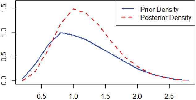
Figure 1 Prior and posterior density.

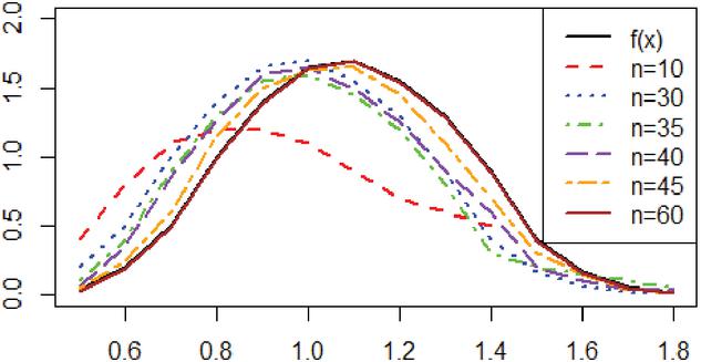
Figure 2 The curve of $f(x;\mu ,\nu ,\theta )$ (Bold) and ${\widehat{f}}_{BS}(x;\mu ,\nu ,\theta )$ (Dotted).

7 Result and Discussion

In order to evaluate the effectiveness of the estimators within the context of SELF with respect to the accurate assessment of reliability, we have illustrated the prior and posterior probability densities in Figure 1. And in Figure 2, we have illustrated the graph ${\widehat{f}}_{BS}(x;\mu ,\nu ,\theta )$ for various values of $n=10,30,35,40,45,60$ within the SELF framework. From the visual representations, it can be inferred that when the value of n increases, then ${\widehat{f}}_{BS}(x;\mu ,\nu ,\theta )$ approaches that of $f(x;\mu ,\nu ,\theta )$. This observation corroborates the consistency property associated with the estimators. For the inverse family of distributions, we employed a Bayesian framework to derive the reliability function. Under the guidance of the general entropy loss function (GELF) and the squared error loss function (SELF), Bayesian estimators for the reliability function and the stress-strength configuration were developed, incorporating the power of the parameter into the evaluation. Bootstrap sampling techniques were used to evaluate the estimator’s effectiveness for $R(t)$. The Bayesian estimator of $R(t)$ was estimated by generating randomized samples of different magnitudes and doing 1000 bootstrap replications for each sample. As can be seen from Table 1, for the reliability function $R(t)$, the Bayesian estimator using the SELF criterion performs superior than its counterpart under the GELF criterion. As the sample size escalates, the estimator under GELF converges toward the performance levels of the estimator using SELF. Furthermore, for different $t$ values, the SELF-based estimator consistently demonstrates a performance advantage over the GELF-based estimator. In contrast, Table 2 illustrates that when $n<m$, the estimator derived under the SELF criterion yields more favorable results than that derived under the GELF criterion. As both $n$ and $m$ increase, the performance metrics of the two estimators become nearly indistinguishable.

Table 1 Estimated values of $R(t)$ for varying $\mathit{n}$

$\mathit{n}$		30		35		40		50		60
t	R(t)	SELF	GELF	SELF	GELF	SELF	GELF	SELF	GELF	SELF	GELF
2	0.8997	0.8749	0.8734	0.8894	0.8889	0.8937	0.8936	0.8984	0.8994	0.8997	0.8997
		-0.0405	-0.0419	-0.0267	-0.0271	-0.0226	-0.0226	-0.0177	-0.0177	-0.0166	-0.0166
		0.00021	0.00021	0.00011	0.00011	0.00011	0.00011	0.00011	0.00011	0.00011	0.00011
		0.0480	0.0518	0.0445	0.0455	0.0385	0.0388	0.0301	0.0301	0.0275	0.0275
		89.4006	89.2958	88.0759	87.8437	86.4375	86.3769	82.8716	82.6226	83.5155	83.4214
2.5	0.8882	0.7307	0.7163	0.7844	0.7778	0.8062	0.8023	0.8425	0.8410	0.8560	0.8554
		-0.1726	-0.1871	-0.1190	-0.1256	-0.0971	-0.1011	-0.0609	-0.0623	-0.0474	-0.0480
		0.0008	0.0009	0.0010	0.0012	0.0008	0.0009	0.0004	0.0005	0.0003	0.0003
		0.1090	0.1162	0.1262	0.1328	0.1133	0.1177	0.0832	0.0851	0.0663	0.0671
		90.1057	90.0781	90.8495	90.8582	90.4125	90.3991	88.5612	88.5699	89.5762	89.5723
3	0.8178	0.5437	0.5171	0.6147	0.5987	0.6463	0.6351	0.7078	0.7019	0.7331	0.7300
		-0.2893	-0.3160	-0.2183	-0.2343	-0.1867	-0.1979	-0.1252	-0.1311	-0.0999	-0.1030
		0.0012	0.0013	0.0021	0.0023	0.0019	0.0020	0.0014	0.0014	0.0009	0.0009
		0.1308	0.1352	0.1744	0.1808	0.1666	0.1718	0.1392	0.1427	0.1165	0.1184
		90.0795	90.0775	91.2916	91.3092	91.2135	91.2227	89.7920	89.8173	90.4307	90.4637
3.5	0.6980	0.3887	0.3589	0.4577	0.4372	0.4895	0.4741	0.5567	0.5470	0.5853	0.5797
		-0.3245	-0.3543	-0.2555	-0.2760	-0.2237	-0.2391	-0.1565	-0.1662	-0.1279	-0.1335
		0.0011	0.0011	0.0022	0.0023	0.0021	0.0022	0.0018	0.0019	0.0013	0.0013
		0.1252	0.1250	0.1777	0.1798	0.1752	0.1775	0.1582	0.1605	0.1373	0.1387
		90.0271	89.9570	91.3067	91.3063	91.3712	91.3821	90.1207	90.1317	90.5907	90.5881
4	0.5707	0.2749	0.2469	0.3353	0.3146	0.3638	0.3476	0.4265	0.4154	0.4537	0.4470
		-0.3110	-0.3390	-0.2506	-0.2713	-0.2221	-0.2383	-0.1594	-0.1705	-0.1322	-0.1389
		0.0008	0.0008	0.0018	0.0018	0.0018	0.0018	0.0017	0.0017	0.0013	0.0013
		0.1115	0.1089	0.1627	0.1614	0.1631	0.1627	0.1539	0.1545	0.1367	0.1372
		89.9613	89.9449	91.2753	91.2588	91.4044	91.4100	90.2110	90.2307	90.6410	90.6334

Table 2 Estimated values of $P$ for varying ${\mathit{\mu }}_{\text{2}}$

${\mathit{\mu }}_{\text{2}}$	2.5		3		3.5		4		4.5
P	0.8032		0.7556		0.7139		0.6771		0.6445
(n,m)	SELF	GELF	SELF	GELF	SELF	GELF	SELF	GELF	SELF	GELF
(25,25)	0.7625	0.7516	0.6565	0.6413	0.6338	0.6177	0.6631	0.6480	0.6221	0.6057
	-0.0740	-0.0849	-0.1324	-0.1476	-0.1134	-0.1295	-0.0474	-0.0624	-0.0556	-0.0720
	0.0034	0.0036	0.0035	0.0036	0.0033	0.0035	0.0026	0.0027	0.0038	0.0039
	0.2473	0.2542	0.2466	0.2524	0.2474	0.2527	0.2176	0.2225	0.2607	0.2663
	90.6778	90.6833	90.0362	90.0580	91.5023	91.4933	91.2506	91.2917	91.1556	91.1658
(25,35)	0.7860	0.7776	0.7221	0.7113	0.6998	0.6882	0.6720	0.6596	0.6558	0.6428
	-0.0505	-0.0589	-0.0668	-0.0775	-0.0474	-0.0590	-0.0384	-0.0509	-0.0219	-0.0349
	0.0029	0.0030	0.0038	0.0040	0.0035	0.0037	0.0043	0.0045	0.0035	0.0036
	0.2315	0.2368	0.2588	0.2649	0.2490	0.2545	0.2778	0.2838	0.2516	0.2566
	91.7116	91.7082	90.3282	90.3481	90.4357	90.4450	91.1105	91.1196	91.0729	91.0695
(35,35)	0.8082	0.8021	0.7223	0.7136	0.7082	0.6992	0.6769	0.6670	0.6623	0.6520
	-0.0283	-0.0343	-0.0666	-0.0752	-0.0390	-0.0480	-0.0335	-0.0435	-0.0154	-0.0258
	0.0036	0.0038	0.0027	0.0028	0.0037	0.0038	0.0032	0.0033	0.0030	0.0031
	0.2529	0.2577	0.2229	0.2269	0.2572	0.2619	0.2378	0.2418	0.2356	0.2393
	90.3527	90.3288	90.7808	90.8115	91.0224	91.0205	89.9200	89.9403	91.3957	91.3809
(35,45)	0.8091	0.8041	0.7805	0.7749	0.7237	0.7167	0.7085	0.7011	0.7047	0.6972
	-0.0274	-0.0323	-0.0084	-0.0140	-0.0235	-0.0305	-0.0019	-0.0093	0.0270	0.0195
	0.0021	0.0021	0.0025	0.0026	0.0028	0.0028	0.0035	0.0036	0.0031	0.0032
	0.1936	0.1963	0.2139	0.2169	0.2223	0.2255	0.2538	0.2576	0.2359	0.2393
	91.2810	91.3250	91.1045	91.0867	90.3049	90.3166	91.3587	91.3561	90.8918	90.8970
(45,45)	0.8112	0.8076	0.8660	0.8633	0.7700	0.7656	0.7156	0.7101	0.7064	0.7008
	-0.0253	-0.0289	0.0771	0.0745	0.0228	0.0184	0.0051	-0.0003	0.0286	0.0230
	0.0022	0.0023	0.0022	0.0023	0.0021	0.0022	0.0026	0.0026	0.0031	0.0032
	0.2025	0.2045	0.2021	0.2041	0.1946	0.1966	0.2161	0.2184	0.2396	0.2422
	91.5000	91.4698	90.8158	90.8117	90.4342	90.4452	90.5356	90.5504	91.5544	91.5457

References

[1] M. Abramowitz and I. A. Stegun, Handbook of Mathematical Functions with Formulas, Graphs, and Mathematical Tables. National Bureau of Standards, 1964.

[2] R. Calabria and G. Pulcini, Point estimation under asymmetric loss functions for left-truncated exponential samples. Communications in Statistics-Theory and Methods, 25(3), 585–600, 1996.

[3] S. Kotz, Y. Lumelskii, and M. Pensky, The stress-strength model and its generalizations: Theory and applications. World Scientific Publishing Co. Pvt. Ltd., 2003.

[4] D. Kundu and R.D. Gupta, Estimation of $P(Y<X)$ for Weibull distributions. IEEE Transactions on Reliability, 55, 270–280, 2006.

[5] I.S. Gradshteyn, I.M. Ryzhik, Tables of Integrals, Series, and Products. Academic Press, New York, 2007.

[6] M.Z. Raqab, M.T. Madi, and D. Kundu. Estimation of $P(Y<X)$ for the three-parameter generalized exponential distribution. Communications in Statistics – Theory and Methods, 37, 2854–2864, 2008

[7] A. Chaturvedi and S. K. Tomer. Classical and Bayesian reliability estimation of the negative binomial distribution. Journal of Applied Statistical Science, 11, 33–43, 2002.

[8] A. Chaturvedi, K. Chauhan, and M.W. Alam. Estimation of the reliability function for a family of lifetime distributions under type I and type II censorings. Journal of Reliability and Statistical Studies, 2(2), 11–30, 2009.

[9] A. Chaturvedi, K. Chauhan. Estimation and testing procedures for the reliability function of the Weibull distribution under type I and type II censoring. Journal of Statistics Sciences, 1(2), 121–136, 2009.

[10] A. Chaturvedi, K. Chauhan, and M.W. Alam. Robustness of the sequential testing procedures for the parameters of zero-truncated negative binomial, binomial, and Poisson distributions. Journal of the Indian Statistical Association, 51(2), 313–328, 2013.

[11] M. Jovanovic, Estimation of $P(X<Y)$ for geometric-exponential model based on complete and censored samples. Communications in Statistics – Simulation and Computation, 46, 3050–3066, 2016

[12] R. Kumari, K.K. Mahajan, and S. Arora. Bayesian estimation of stress-strength reliability using upper record values from a generalized inverted exponential distribution. Engineering and Management Sciences, 4(4), 882–894, 2019.

[13] A.K. Mahto, Y. M. Tripathi, and F. Kızılaslan. Estimating reliability in a multicomponent stress–strength model for a general class of inverted exponentiated distributions under progressive censoring. Journal of Statistical Theory and Practice, 14(4), 2020.

[14] S. Saini, S. Tomer, and R. Garg. On the reliability estimation of a multicomponent stress–strength model for Burr XII distribution using progressively first-failure censored samples. Journal of Statistical Computation and Simulation, 92(4), 667–704, 2021.

[15] V. Agiwal. Bayesian estimation of stress-strength reliability from inverse Chen distribution with application to failure time data. Annals of Data Science, 10(2), 317–347, 2021.

[16] K.S. Chauhan. Estimation and testing procedures of reliability $P(Y<X)$ for the inverse distributions family under type-II censoring. Reliability: Theory and Applications, 17 (3(69)), 328–339, 2022.

[17] A.S. Sarah, Y.H. Ali. Bayesian estimation of reliability for a multicomponent stress-strength model based on the Topple-Leone distribution. Wasit Journal for Pure Sciences, 1(3), 90–104, 2022.

[18] Z. Liming, Xu. Ancha, An. Liuting, Li. Min. Bayesian inference of system reliability for a multicomponent stress-strength model under Marshall-Olkin Weibull distribution. Systems, 10(6):196–196, 2022.

[19] S. Saini, R. Garg. Non-Bayesian and Bayesian estimation of stress-strength reliability from Topp-Leone distribution under progressive first-failure censoring. International Journal of Modelling and Simulation, 44(1), 1–15 2022.

[20] A. Abdulhakim, Al. Babtain, E. Ibrahim, M. A. Ehab. Bayesian and non-Bayesian reliability estimation of the stress-strength model for the power-modified Lindley distribution. Computational Intelligence and Neuroscience, 2022(1), 1154705, 2022.

[21] S. Saini, S. Tomer, and R. Garg. Inference of multicomponent stress-strength reliability following Topp-Leone distribution using progressively censored data. Journal of Applied Statistics, 50(7), 1538–1567, 2022.

[22] R. Mahdi, S. Mohamed, M. Y. Haitham, and E. A. Ali. Estimating the multicomponent stress-strength reliability model under the Topp-Leone distribution: applications, Bayesian and non-Bayesian assessment. Statistics, Optimization and Information Computing, 12(1), 133–152, 2023.

[23] K. Zahra, E.G. Yari. Bayesian estimation of the stress-strength reliability based on generalized order statistics for the Pareto distribution. Journal of Probability and Statistics, 2023(1), 8648261, 2023.

[24] K.S. Chauhan, A. Sharma. Estimation Sequential Testing Procedure for the Parameters of the Inverse Distributions Family. Reliability: Theory and Applications, 19(1(77)), 819–831, 2024.

[25] Ma. Haijing, Jia. Mei. Jun, Peng. Xiuyun, Yan. Zaizai. Objective Bayesian estimation for the multistate stress-strength model’s reliability with various kernel functions. Quality and Reliability Engineering International, 40(5), 2776–2791, 2024.

Biographies

Kuldeep Singh Chauhan is an assistant professor in the Department of Statistics at Ram Lal Anand College, University of Delhi, India. He holds a Ph.D. in Statistics, specializing in Reliability and Life Testing, awarded by Chaudhary Charan Singh University, Meerut. With over 14 years of teaching experience, He has published more than seven research papers in reputed journals.

Sachin Tomer is an associate professor in the Department of Statistics at Ramanujan College, University of Delhi, India. He has more than 15 years of teaching experience. Dr. Tomer completed his Ph.D. in Statistics in Reliability and Life Testing from Chaudhary Charan Singh University, Meerut. His research interests include Bayesian inference and reliability, and life testing. He has published more than 15 research papers in reputed journals.

Journal of Reliability and Statistical Studies, Vol. 19, Issue 2 (2026), 241–262
doi: 10.13052/jrss0974-8024.1921
© 2026 River Publishers