Stochastic Analysis of Redundant RF Amplifiers with Priority Repair and Data-Driven Parameters

Yogita Rani^{1, 3}, Gitanjali^2,* and Indeewar Kumar³

¹Department of Applied Sciences, BPIT, GGSIPU, Delhi, India
²Department of Applied Sciences, MSIT, GGSIPU, Delhi, India
³Department of Mathematics and Statistics, Manipal University Jaipur, Jaipur, India
E-mail: yogita.tiwary@gmail.com; yogita.211051039@muj.manipal.edu; drgitanjali@msit.in; geetumongia@gmail.com; indeewar.kumar@jaipur.manipal.edu; indeewar.kum@gmail.com
*Corresponding Author

Received 17 September 2025; Accepted 03 August 2026

Abstract

RF amplifier modules provide fundamental and indispensable functionality across diverse domains such as aerospace, defence, medical imaging, industrial automation, and scientific research by ensuring reliable operation and robust signal transmission. Their criticality is amplified in high-end applications for example cellular base stations, radar, and real-time networks dependent. The current work develops a stochastic model for the reliability analysis of a parallel redundant system comprising a primary and a backup RF Power Amplifier Module. Utilizing the semi-Markov Regenerative Point Technique (SMRPT), we compute key metrics like Mean Time to System Failure (MTSF), availability and system’s profit. The system is initially fully operational and fails only when both units fail. A dedicated server performs immediate, flawless repairs upon failure, prioritizing the primary module. The study assumes constant failure rates and exponentially distributed repair times. To estimate the failure and repair rates from empirical data, a linear regression technique which is one of the fundamental supervised learning methods in AI and machine learning, is utilized. The observed repair and failure times are considered as dependent variables and the rates are approximated as the inverse of the mean observed times.

Keywords: Parallel systems, RF power amplifier module, RF backup amplifier module, reliability analysis, and regenerative point technique and semi-Markov process.

1 Introduction

Every industry uses cutting-edge technology, which drives the need for complicated systems. In industrial and manufacturing processes, complex systems are made up of numerous units, subsystems, or systems that are arranged in parallel, series, or a mix of these. It becomes essential to measure the reliability of these systems in order to get optimal performance and guarantee efficiency. Numerous researchers have conducted in-depth studies to gauge the reliability of different systems with a range of configurations over the years. For example, Lado and Singh [2] and Singh developed models for repairable systems with subsystems connected in series. Kumar et al. [11, 12] investigated the reliability of dragline subsystems arranged in series. Li et al. [37] discussed the reliability of series systems with Weibull-distributed components and utilized minimum lifetime distribution theory. While these studies focus on series-connected repairable systems, the other configurations also exist in real-world applications. Kumar and Kumar [23] developed a quantitative model for a smart trash bin with six components in series. This study focused on providing repair and maintenance activities for prolonged availability.

Additionally, there are certain systems that are non-repairable, where failed components are not restored but discarded or replaced entirely. Few studies have addressed such systems; for instance, Jaiswal et al. [21] developed models for non-repairable complex systems, where subsystems follow weighted k-out-of-n: G configurations and are joined in series, using the universal generating function approach. In such arrangements, system stops functioning only when a critical series unit fails without redundancy or when all parallel paths inside a stage fail. This configuration is frequently used to enhance overall system reliability. Surapati et al. [28] developed an integrated series-parallel system model and examined the impact of various operational constraints using a dynamic programming approach. Todinov [18] conducted a study aimed at improving the reliability of series-parallel systems through reverse engineering of valid algebraic inequalities, providing novel strategies to identify weak spots and improve system design. Kumar [3] and Kundu et al. [33] analysed the reliability of repairable system by incorporating detection delays, imperfect coverage, and parameter uncertainty using Bayesian and optimization techniques.

Building on the insight that stage-wise redundancy provides one avenue of design, and related research exclusively focuses on fully parallel systems. Gitanjali [14] and Malik and Gitanjali [29] performed stochastic analyses of identical-unit parallel systems. Kumar and Ram [4] studied the reliability analysis of a urea fertilizer plant using supplementary variable technique. Kommula and Mishra [7] modelled a three-unit identical system with two independent failure modes and obtained reliability estimates via maximum-likelihood estimation, while Singh et al. [8] adopted a Bayesian framework for a two-unit identical parallel system with expert and regular repair facilities under geometric failures. Heterogeneous (non-identical) parallels systems have likewise been studied: Kadyan and Malik [31] and Gitanjali and Malik [15] analysed repairable machine assemblies, and Al. Ammouri et al. [1] together with Badola et al. [22] quantified reliability metrics for two-unit systems subject to distinct failure modes. Lawan et al. [19] analyzed a dissimilar parallel system with two repair machines with numerical experiments. Shekhar et al. [9], studied standbys provision for machine repair problem in a Markovian environment with unreliable service and vacation interruption.

Series, parallel, and series-parallel arrangements have their dominance in conventional reliability structures, but contemporary systems demands more dynamic and versatile approaches. Consequently, the concept of k-out-of-n: G systems evolved, enabling a system to function properly as long as k of the n components are in working order. These systems offer more modeling fidelity in practical applications and generalize the binary working-failed condition. Munjal and Singh [6], Ramesh and Gupta [17], examined systems with parallel-connected subsystems under the k-out-of-n: G policy using stochastic techniques. Krishnan [27] studied the reliability assessment of k-out-of-n: G weighted systems and applied the model to domains such as wireless sensor networks, high-altitude unmanned platforms, and unmanned aerial vehicles (UAVs). In another advancement, Wang et al. [10] developed a model for dynamic k-out-of-n phase-AND systems by integrating combinatorial logic with decision-diagram-based methods, further expanding the analytical toolkit for reliability assessment in complex system architectures. Other research has examined complex systems focusing on the reliability of subsystems. Kumar et al. [5] and Saini et al. [20] studied systems like the Sludge digestion processing system and the Load haul dump system using a Genetic algorithm approach. Rani et al. [35, 36] studied a parallel heat exchanger and a centrifugal pump system using SMPRT. The stochastic modeling of Wireless Sensor Networks by markov model and particle swam optimization is presented by Jadhav and Kumar [30].

In today’s communication system, which ranges from radar systems and satellite communication configurations to cellular base stations and broadcasting equipment, Radio Frequency (RF) Power Amplifier Modules facilitate the efficient transmission of signals across long distances. Continuous performance is critical expectation from these modules, even amidst variable electrical loads and diverse environmental stresses. To mitigate disruptions in mission-critical communication tasks, RF systems employ a parallel setup of primary and backup amplifiers, ensuring redundancy and fault tolerance. Despite the essential role of these setups in system reliability, very few studies have been conducted in this area. Even design-based methods to enhance reliability of RF system, such as Ferreira et al. [25], who proposed the reliability-oriented design methods for RF front-end systems. Mitra et al. [13] investigated the impacts of substrate thinning on the output power, phase noise, and the frequency stability of RF performance in VCO chips. Kaul and Dey [32] proposed design advice for enhancing reliability by analysing failure reasons in RF MEMS switches and phase shifters for up to one billion cycles.

Although prior research focus on general repairable or redundant systems, the specific failure-repair-priority processes and probabilistic downtime characteristics of RF modules are rarely captured. Hence, this study undertakes a comprehensive stochastic examination of a parallel configuration consisting of a primary and backup RF Power Amplifier Module. Both are initially active, and as long as at least one of them is operational, the system functions. When a system malfunctions, it is immediately fixed, with the first system being repaired first. To fully examine and model complex systems, the study uses cutting-edge approaches like the RPT and the SMP for assessment of metrics including mean time to system failure, availability, and revenue function. Lévy [24] introduced the SMP. Sur [26] made a substantial contribution to the formal advancements of SMP theory. The pioneer work for the regeneration point technique was established by Feller [34] in his renewal theory. The regeneration point technique was used in dependability and queuing theory by Neyman and Scott [16].

Structure of Paper

The organization of the paper is as follow. Section 2. Methodology: To analyse the constructed model with overall strategy employed, is presented in the flowchart, as illustrated in Figure 1. The semi-Markov process and the regenerative point technique, the two principal analytical approaches to study the developed model are introduced in this section. Section 3. Case Study: A real-world case study of an RF Amplifier Module is provided to demonstrate the practical utility of the developed model. Section 4. System Description: This section describes the system configuration with its main units, as shown in Figure 1 block diagram. Section 5. Analysis: This section presents the notations used in this study (as detailed in Table 1), the state descriptions (as mention in Table 2) and the computation of transition probabilities, mean sojourn times, availability, and profit required for assessing the system performance. Section 6. Results and Discussions: The results obtained from all the numerical calculations are discussed in this section. Section 7. Conclusion: To summarize key insights for system reliability, the final conclusion is present in this section. Section 8. Limitation and future scope: This section describes limitation and future scope of this work.

2 Methodology

This study conducted the stochastic analysis of a parallel system consisting of an RF power amplifier module and an RF backup module, utilising a combined approach of the semi-Markov Process (SMP) alongwith the Regenerative Point Technique (RPT). The model of the system in states such as operational, failed, and under repair, with transitions governed by exponential distributions is developed by SMP while identification of regenerative points where the system probabilistically resets simplifying the evaluation of long-term performance. This integrated approach is applied to assess reliability metrics encompassing Mean Time to System Failure (MTSF), availability, and profit by recurrence relations and Laplace-Stieltjes transforms which provides a robust framework for assessing system performance.

System States: The system is modelled by a finite state space $S=\{S_0,S_1,S_2,\mathrm{\dots },S_n\}$, where each state $S_i$ corresponds to a specific operational or failure condition. The transition from state $S_i$ to state $S_j$ are characterised by the transition rate $q_{ij}$ of the generator matrix.

Semi-Markov Process: Let $\{X(t),t\ge 0\}$ be a stochastic process with state space $S$. This process called a semi-Markov process if the embedded sequence $\{X_n\}$ is a markov chain with transition probabilities matrix $P_{ij}$. The transition probability $P_{ij}=P(X_{n+1=j}|X_{n=i}),i,j\in S$. The time spent in state $i$ before transition to state $j$ is a random variable that follows distribution function $Q_{ij}(t)=P(T_{ij}\le t)$. If the sojourn times are exponentially distributed with parameter ${\lambda }_i$, i.e., $Q_{ij}=1-e^{-{\lambda }_i(t)}$, the semi-Markov process becomes a continuoustime stochastic process.

Regenerative Point Technique: In stochastic process theory, a time $t=\tau$ is called a regenerative point if the process regenerates at $\tau$, independent of the past.

Steady State Availability: For a repairable system considering constant failure and repair rates, the availability is defined as:

$$A=\frac{\mathit{MTTF}}{\mathit{MTTF}+\mathit{MTTR}}=\frac{\mu }{\lambda +\mu }\text{where}\lambda =\text{Failure}$$

Rate, $\mu =$ Repair Rate, MTTF $=$ Mean Time to Failure, MTTR $=$ Mean Time to Repair.

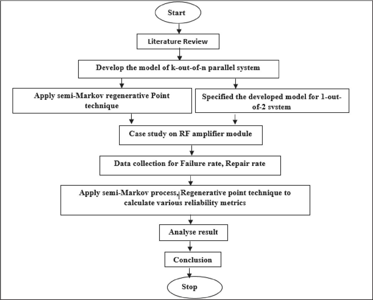
Figure 1 Methodology for RF amplifier system.

Mean Time to System Failure: Let $\{X(t)\}\in S,t\ge 0$ be a stochastic process with finite state space $S$, and let $F\subset S$, be the set of failed state then time to system failure is defined as $T=inf\{t>0:X(t)\in F\}$. The Mean Time to System Failure is given as MTSF $E[T]=$ ${\int }_0^{\mathrm{\infty }}R(t)\mathit{d}t$, where $R(t)$ the reliability function is, $R(t)=P(T>t)$

• Detailed literature review on reliability models of various systems comprising units, subsystems, and systems arranged in parallel, series, series-parallel, and k-out-of-n configurations.

• Applied a k-out-of-n model, focusing on the 1-out-of-2 case.

• The current work uses the semi-Markov process in association with Regenerative Point Technique as the primary analytical tools.

semi-Markov processes: A semi-Markov process is considered a stochastic model that allows state holding times to follow general probability distributions which is unlike Markov processes, where state durations follow an exponential law. This property makes semi-Markov processes more suitable for modeling complex systems to represent real-world stochastic systems for our analysis. The study of semi-Markov processes was initially presented by Lévy [24], and later notable theoretical advancements contributed by Sur [26].

Regenerative point technique: In probability theory, a regenerative process is a stochastic process in which the system probabilistically restarts itself at certain random times, called regenerative point. At these times, the forthcoming state of the process is free from the past and follows the same probability law as the original process. In renewal theory, Feller [36], laid the groundwork for the regenerative point technique, which was further applied by Neyman and Scott [16] in queuing and reliability analysis.

3 Case Study

To depict the practical relevance of the constructed reliability model, a field study on RF Amplifier Modules is described in this section.

3.1 Layout of RF Amplifier Module

RF Amplifier module is one of the most crucial highfrequency electronic systems. It serves a pivotal role in modern communication systems, defense, applications, and aerospace. The present study proposed a reliability model for an RF amplification comprising two systems: first system (${\mathrm{H}}_1$), the RF Power Amplifier Module configured in parallel with second system (${\mathrm{H}}_2$), the RF Backup Amplifier Module. To achieve steady and dependable signal amplification in mission-oriented scenarios, these modules are essential.

RF Power Amplifier Module (First system ${\mathbf{H}}_{\mathbf{1}}$): The RF Power Amplifier Module employed as primary component in charge of amplifying RF signals to reach the appropriate output level. It ensures high gain amplification in areas with long-distances. It is frequently used in real-time application with priority due to its exceptional performance.

RF Backup Amplifier Module (Second system ${\mathbf{H}}_{\mathbf{2}}$): In case of failure and maintenance requirement, the RF Backup Amplifier Module operates as a standby unit. It is structured with similar electrical conditions as those of main amplifier (${\mathrm{H}}_1$) to ensure smooth transition with minimum signal disruption. In the reliability examination of the entire system, a crucial role is played by this system $({\mathrm{H}}_2)$ with repair characteristics.

4 System Description

The study developed a complex reliability model for an RF amplification system designed with two systems, ${\mathrm{H}}_1$ and ${\mathrm{H}}_2$. Each system, comprised of a single unit, is connected in parallel as shown in Figure 2.

Assumptions:

• Either of the two systems is sufficient for the overall functioning of the system.

• The system always has one server available. After a failure, the unit of the system undergoes for repair, with priority to repair first system.

• The repair time is exponential. Failure rates of the units are constant.

• Repair times and failure times are independent and identically distributed (i.i.d.) random variables.

• Rate estimators are obtained using the inverse of the sample mean.

• The linear regression framework assumed that the observed times vary randomly about the theoretical mean, subject to independent error having zero mean.

• The error term in the regression representation reflects random stochastic variability and is not assumed to be normally distributed.

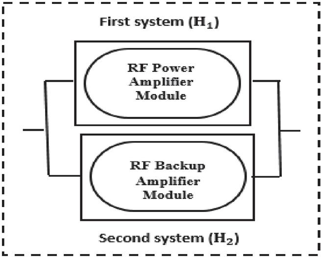
Figure 2 Block diagram.

5 Analysis

The reliability analysis are discussed in this section, showing how system performance is affected by repair and failure rates. Various reliability measures namely Mean Time to System Failure (MTSF), availability, and profit across are assessed through the semi-Markov Process with the Regenerative Point Technique. The findings of the results are interpreted through numerical and qualitative perspectives.

5.1 Notations

The notations used throughout the analysis to understand the system model, are detailed in the Table 1. These notations represent the two parallel system: RF Power Amplifier Module and RF Backup Amplifier Module, components, functional and failure states, repair and failure rates, probability distributions, and other functions necessary for the stochastic modeling of the RF Power Amplifier Module and its Backup.

Table 1 Notations

Notations:	Notations Description
${\mathrm{H}}_1/{\mathrm{H}}_2$	RF Power Amplifier Module/RF Backup Amplifier Module
A	The unit of RF Power Amplifier Module
B	The unit of RF Backup Amplifier Module
${\mathrm{H}}_1\mathrm{O}/{\mathrm{H}}_2\mathrm{O}$	RF Power Amplifier Module/RF Backup Amplifier Module is in operational state.
$\overline{{\mathrm{H}}_1}\mathrm{AUr}$	RF Power Amplifier Module is under repair due to failure of unit A.
${\mathrm{H}}_2\mathrm{BUr}$	RF Backup Amplifier Module is under repair due to failure of unit B.
${\overline{\mathrm{H}}}_1{\mathrm{AU}}_{\mathrm{R}}$	RF Power Amplifier Module is under repair continuously from preceding state due to failure of unit A.
${\mathrm{H}}_2{\mathrm{BW}}_{\mathrm{r}}$	RF Backup Amplifier Module is failed due to failure of unit B and waiting for repair.
${\tau }_1/{\tau }_2$	fixed failure rate of unit A/unit B.
$\alpha /\beta$	fixed repair rate of unit A/unit B.
${\mathrm{g}}_1(\mathrm{t})/{\mathrm{G}}_1(\mathrm{t})$	p.d.f/c.d.f. of the repair time for RF Power Amplifier Module $({\mathrm{H}}_1)$.
${\mathrm{g}}_2(\mathrm{t})/{\mathrm{G}}_2(\mathrm{t})$	p.d.f/c.d.f. of the repair time for RF Backup Amplifier Module $({\mathrm{H}}_2)$.
${\mathrm{r}}_{\mathrm{ij}}(\mathrm{t})/{\mathrm{R}}_{\mathrm{ij}}(\mathrm{t})$	p.d.f. /c.d.f. of transition period from regenerative state i to a state j or to a non-functioning state j without passing any other regenerative state in (0, t].
${\mathrm{m}}_{\mathrm{ij}}$	When system transits straight to state ${\mathrm{S}}_{\mathrm{i}}$, contribution to mean sojourn time ${\mu }_{\mathrm{i}}$ in state ${\mathrm{S}}_{\mathrm{i}}$ so that ${\mu }_{\mathrm{i}}={\sum }_{\mathrm{j}}{\mathrm{m}}_{\mathrm{ij}}$ where ${\mathrm{m}}_{\mathrm{ij}}=\int {\mathrm{tdQ}}_{\mathrm{ij}}(\mathrm{t})=-{\mathrm{q}}_{\mathrm{ij}}^{\ast }(0)$
${\mu }_{\mathrm{i}}$	Mean sojourn time in state ${\mathrm{S}}_{\mathrm{i}}$ which is given by ${\mu }_{\mathrm{i}}=\mathrm{E}\left({\mathrm{T}}_{\mathrm{i}}\right)={\int }_0^{\mathrm{\infty }}\mathrm{P}({\mathrm{T}}_{\mathrm{i}})\mathrm{dt}={\sum }_{\mathrm{j}}{\mathrm{m}}_{\mathrm{ij}}$ where ${\mathrm{T}}_{\mathrm{i}}$ notate the time to failure.
*/*	Laplace Stieltjes transform/Laplace transform.
$\otimes /\mathrm{\circledR }$	Stieltjes convolution/Laplace convolution.

5.2 Description of States

The proposed model is designed using several states (designated as $S_{0,}{S}_1,S_2,S_3,S_4$) as detailed in Table 2. States ($S_0,S_1,S_2$) represents the up-states whereas the states ($S_3,S_4$) are failed states. Every state reflects the operating condition of both system, caused by the working condition of the respective unit.

Table 2 States of system

States	State Description
${\mathrm{S}}_0$	An up state where RF Power Amplifier Module $({\mathrm{H}}_1)$ and RF Backup Module $({\mathrm{H}}_2)$ are operational.
${\mathrm{S}}_1$	An up state where RF Power Amplifier Module $({\mathrm{H}}_1)$ is not operating due to failure of unit A and under repair while RF Backup Module $({\mathrm{H}}_2)$ is operative.
${\mathrm{S}}_2$	An up state where RF Backup Amplifier Module $H_2$ is not operating due to failure of unit B and under repair while RF Power Amplifier Module $({\mathrm{H}}_1)$ is operative.
${\mathrm{S}}_3$	A failed state where RF Backup Amplifier Module (${\mathrm{H}}_2$) is not operating due to failure of unit B and waiting to get repair while RF Backup Amplifier Module ${\mathrm{H}}_1$ is continuously being repaired from its previous state.
${\mathrm{S}}_4$	A failed state where RF Power Amplifier Module ${\mathrm{H}}_1$ is not operating due to failure of unit A and waiting to get repair while RF Backup Amplifier Module ${\mathrm{H}}_2$ is continuously being repaired from its previous state.

The state transition diagram used to develop the reliability model for the RF power amplifier system and the RF backup amplifier system is illustrated in Figure 3. The diagram is classified into two categories: operational states (denoted by pink circles) and failed states (denoted by green squares). Transitions from one state to another are shown using arrows, annotated with failure rates $({\tau }_1/{\tau }_2)$ and the probability density function $g_i(t)$ of the repair time. Some arrows terminate at a regenerative point (represented by a small black circle), indicating that the system may restart probabilistically from that point.

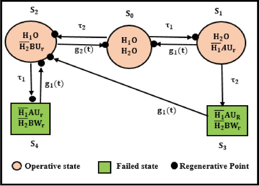
Figure 3 State transition diagram.

5.3 Steady State Transition Probabilities and Mean Sojourn Times

The formula for transition probabilities of various steady states as defined in Table 1, are as follows:

$${\mathrm{p}}_{\mathrm{ij}}={\mathrm{R}}_{\mathrm{ij}}(\mathrm{\infty })={\int }_0^{\mathrm{\infty }}{\mathrm{r}}_{\mathrm{ij}}(\mathrm{t})\mathrm{dt}$$	(1)
$${\mathrm{dR}}_{\mathrm{ij}}(\mathrm{t})={\mathrm{r}}_{\mathrm{ij}}(\mathrm{t})\mathrm{dt}$$	(2)
$${\mathrm{dR}}_{01}(\mathrm{t})={\mathrm{r}}_{01}(\mathrm{t})\mathrm{dt}={\tau }_1{\mathrm{e}}^{-\left({\tau }_1+{\tau }_2\right)\mathrm{t}}\mathrm{dt}.$$	(3)

Taking LST of above equation we get,

$${\mathrm{R}}_{01}^{\ast \ast }(\mathrm{s})={\int }_0^{\mathrm{\infty }}{\mathrm{e}}^{-\mathrm{st}}\mathrm{d}\left[{\mathrm{R}}_{01}(\mathrm{t})\right]={\tau }_1{\int }_0^{\mathrm{\infty }}{\mathrm{e}}^{-\left({\tau }_1+{\tau }_2+s\right)\mathrm{t}}\mathrm{dt}=\frac{{\tau }_1}{{\tau }_1+{\tau }_2+s}.$$

(4)

Now as $\mathrm{s}\to 0$ then we get steady state probability

$${\mathrm{p}}_{01}=\frac{{\tau }_1}{{\tau }_1+{\tau }_2}.$$

(5)

Likewise, steady state transition probabilities can be obtained as follow:

$${\mathrm{p}}_{02}=\frac{{\tau }_2}{{\tau }_1+{\tau }_2}$$	(6)
$${\mathrm{p}}_{10}={\mathrm{g}}_1^{\ast }\left({\tau }_2\right)$$	(7)
$${\mathrm{p}}_{13}=1-{\mathrm{g}}_1^{\ast }\left({\tau }_2\right)$$	(8)
$${\mathrm{p}}_{20}={\mathrm{g}}_2^{\ast }\left({\tau }_1\right)$$	(9)
$${\mathrm{p}}_{24}=1-{\mathrm{g}}_2^{\ast }\left({\tau }_1\right)$$	(10)
$${\mathrm{p}}_{42}={\mathrm{g}}_1^{\ast }(0)$$	(11)
$${\mathrm{p}}_{32}={\mathrm{g}}_1^{\ast }(0)$$	(12)

It is evident that

${\mathrm{p}}_{01}+{\mathrm{p}}_{02}={\mathrm{p}}_{10}+{\mathrm{p}}_{13}={\mathrm{p}}_{20}+{\mathrm{p}}_{24}={\mathrm{p}}_{10}+{\mathrm{p}}_{1,2:3}={\mathrm{p}}_{20}+{\mathrm{p}}_{2,2:4}=1.$

(13)

${\mu }_i$, the mean sojourn time, is obtained as:

${\mu }_0$	$={\mathrm{m}}_{01}+{\mathrm{m}}_{02}={\displaystyle \frac{1}{{\tau }_1+{\tau }_2}},{\mu }_1={\mathrm{m}}_{10}+{\mathrm{m}}_{13}={\displaystyle \frac{1}{\alpha +{\tau }_2}},$
${\mu }_2$	$={\mathrm{m}}_{20}+{\mathrm{m}}_{24}={\displaystyle \frac{1}{\beta +{\tau }_1}},{\mu }_1^{\prime }={\mathrm{m}}_{10}+{\mathrm{m}}_{1,2:3}={\displaystyle \frac{1}{\alpha }},$
${\mu }_2^{\prime }$	$={\mathrm{m}}_{20}+{\mathrm{m}}_{2,1:4}={\displaystyle \frac{\alpha +{\tau }_1}{\left(\beta +{\tau }_1\right)\alpha }}$	(14)

5.4 Mean Time to System Failure

Here, ${\varphi }_i(\mathrm{t})$ notates the cumulative distribution function (c.d.f.) of the initial time interval between any failure state and the regeneration state. The following recurring relationships are listed below.

${\varphi }_0(\mathrm{t})={\mathrm{R}}_{01}(\mathrm{t})\otimes {\varphi }_1(\mathrm{t})+{\mathrm{R}}_{02}(\mathrm{t})\otimes {\varphi }_2(t).$	(15)
${\varphi }_1(\mathrm{t})={\mathrm{R}}_{10}(\mathrm{t})\otimes {\varphi }_0(\mathrm{t})+{\mathrm{R}}_{13}(\mathrm{t}).$	(16)
${\varphi }_2(\mathrm{t})={\mathrm{R}}_{20}(\mathrm{t})\otimes {\varphi }_0(\mathrm{t})+{\mathrm{R}}_{24}(t).$	(17)

Employing L.S.T. to the above equations, find ${\varphi }_0^{\ast \ast }(\mathrm{s})$, MTSF is given by:

$$\mathrm{MTSF}=\underset{\mathrm{s}\to 0}{lim}\frac{1-{\varphi }_0^{\ast \ast }(\mathrm{s})}{\mathrm{s}}=\frac{{\mathrm{N}}_0}{{\mathrm{D}}_0}.$$

(18)

where

${\mathrm{N}}_0={\mu }_0+{\mathrm{p}}_{01}{\mu }_1+{\mathrm{p}}_{02}{\mu }_2\text{and}{\mathrm{D}}_0=1-{\mathrm{p}}_{01}{\mathrm{p}}_{10}-{\mathrm{p}}_{02}{\mathrm{p}}_{20}.$

(19)

5.5 Availability

Considering the system attains the regeneration state $S_i$ at time $\mathrm{t}=0$, let $A_i(\mathrm{t})$ notates the probability that the system is in the upstate at time t. The recurring relations for $A_i(\mathrm{t})$ are as follow:

$A_0(t)=M_0(t)+r_{01}(t)\mathrm{\circledR }{A}_1(t)+r_{02}(t)\mathrm{\circledR }{A}_2(t).$	(20)
$A_1(t)=M_1(t)+r_{1,2:3}(t)\mathrm{\circledR }{A}_2(t)+r_{10}(t)\mathrm{\circledR }{A}_0(t).$	(21)
$A_2(t)=M_2(t)+r_{2,2:4}(t)\mathrm{\circledR }{A}_2(t)+r_{20}(t)\mathrm{\circledR }{A}_0(t).$	(22)

Where

${\mathrm{M}}_0(\mathrm{t})={\mathrm{e}}^{-\left({\tau }_1+{\tau }_2\right)\mathrm{t}}$	(23)
${\mathrm{M}}_1={\mathrm{e}}^{-\left({\tau }_2\right)\mathrm{t}}\overline{G_1(t)}$	(24)
${\mathrm{M}}_2={\mathrm{e}}^{-\left({\tau }_1\right)\mathrm{t}}\overline{G_2(t)}$	(25)

On employing the Laplace transform and Cramer’s rule to the above equations, the system’s availability ${\mathrm{A}}_0^{\ast }(\mathrm{s})$ in steady state is as follows:

$$A=\underset{t\to \mathrm{\infty }}{lim}{A}_i(t)=\underset{s\to 0}{lim}s{A}_0^{\ast }(s)=\frac{N_A}{D_A}.$$

(26)

where

${\mathrm{N}}_{\mathrm{A}}$	$={\mu }_0\left({\mathrm{p}}_{2,2:4}-1\right)+{\mu }_1\left({\mathrm{p}}_{01}\left({\mathrm{p}}_{2,2:4}-1\right)\right)+{\mu }_2\left({\mathrm{p}}_{02}+{\mathrm{p}}_{01}\left({\mathrm{p}}_{2,2:4}-1\right)\right).$	(27)
${\mathrm{D}}_{\mathrm{A}}$	$={\mu }_0\left({\mathrm{p}}_{2,2:4}-1\right)+{\mu }_1^{\prime }\left({\mathrm{p}}_{01}\left({\mathrm{p}}_{2,2:4}-1\right)\right)+{\mu }_2^{\prime }\left({\mathrm{p}}_{02}+{\mathrm{p}}_{01}\left({\mathrm{p}}_{2,2:4}-1\right)\right).$	(28)

5.6 Server Busy Period Due to Repair

Upon the system enters the regenerative state $S_i$ at $\mathrm{t}=0$, let $B_i(\mathrm{t})$ notates the probability that the technician is performing the repair at an instant t. The recursive relations for $B_i(\mathrm{t})$ are as follows:

${\mathrm{B}}_0(\mathrm{t})={\mathrm{r}}_{01}(\mathrm{t})\mathrm{\circledR }{\mathrm{B}}_1(\mathrm{t})+{\mathrm{r}}_{02}(\mathrm{t})\mathrm{\circledR }{\mathrm{B}}_2(t).$	(29)
${\mathrm{B}}_1(\mathrm{t})={\mathrm{W}}_1(\mathrm{t})+{\mathrm{r}}_{1,2:3}(\mathrm{t})\mathrm{\circledR }{\mathrm{B}}_2(\mathrm{t})+{\mathrm{r}}_{10}(\mathrm{t})\mathrm{\circledR }{\mathrm{B}}_0(t).$	(30)
${\mathrm{B}}_2(\mathrm{t})={\mathrm{W}}_2(\mathrm{t})+{\mathrm{r}}_{2,2:4}(\mathrm{t})\mathrm{\circledR }{\mathrm{B}}_2(\mathrm{t})+{\mathrm{r}}_{20}(\mathrm{t})\mathrm{\circledR }{\mathrm{B}}_0(t).$	(31)

where

${\mathrm{W}}_1(\mathrm{t})={\mathrm{e}}^{-{\tau }_2\mathrm{t}}\overline{G_1(t)}+\left({\tau }_2{\mathrm{e}}^{-{\tau }_2\mathrm{t}}\mathrm{\circledR }1\right)\overline{G_1(t)}.$	(32)
${\mathrm{W}}_2(\mathrm{t})={\mathrm{e}}^{-{\tau }_1\mathrm{t}}\overline{G_2(t)}+\left({\tau }_1{\mathrm{e}}^{-{\tau }_1\mathrm{t}}\mathrm{\circledR }1\right)\overline{G_2(t)}.$	(33)

By applying the Laplace transform to the above set of equations (29)–(33), and using Cramer’s rule, the period of time the technician will be busy while being repaired ${\mathrm{B}}_0^{\ast }(\mathrm{s})$, in a steady state is as follow

$${\mathrm{B}}_0(\mathrm{\infty })=\underset{\mathrm{s}\to 0}{lim}{\mathrm{sB}}_0^{\ast }(\mathrm{s})=\frac{{\mathrm{N}}_{\mathrm{B}}}{{\mathrm{D}}_{\mathrm{A}}}.$$

(34)

where

${\mathrm{N}}_{\mathrm{B}}={\mathrm{W}}_1^{\ast }({\mathrm{p}}_{01}({\mathrm{p}}_{01}({\mathrm{p}}_{2,2:4}-1)))+{\mathrm{W}}_2^{\ast }({\mathrm{p}}_{01}(({\mathrm{p}}_{1,2:3}-1)))+{\mathrm{W}}_2^{\ast }{\mathrm{p}}_{02}$

(35)

and ${\mathrm{D}}_{\mathrm{A}}$ is already established.

5.7 Expected Number of Visit of the Server

At the regenerative state $S_i$, let $V_i(t)$ notates the anticipated number of the visits by the technician in ($0,\mathrm{t}$ ]. The following recurrence relations for $V_i(t)$ are obtained:

$V_0(t)=R_{01}(t)\otimes \left(V_1(t)+1\right)+R_{02}(t)\otimes \left(V_2(t)+1\right).$	(36)
$V_1(t)=R_{1,2:3}(t)\otimes V_2(t)+R_{10}(t)\otimes V_1(t).$	(37)
$V_2(t)=R_{2,2:4}(t)\otimes V_2(t)+R_{20}(t)\otimes V_0(t).$	(38)

Taking L.S.T of Equations (36)–(38) and solving for ${\mathrm{V}}_0^{\ast \ast }(\mathrm{s})$, we get the expected number of visits as

$${\mathrm{V}}_0=\underset{s\to 0}{lim}s{\mathrm{V}}_0^{\ast \ast }(\mathrm{s})=\frac{{\mathrm{N}}_{V_i}}{{\mathrm{D}}_{\mathrm{A}}},$$

(39)

where

$${\mathrm{N}}_{V_i}=({\mathrm{p}}_{01}+{\mathrm{p}}_{02})(1-{\mathrm{p}}_{10})(1-{\mathrm{p}}_{2,2:4}).$$

(40)

5.8 Expected Number of Repairs

On system occupies the regenerative state $S_i$ at $\mathrm{t}=0$, let $R{P}_i(t)$ notates the anticipated number of repairs by the technician in $(0,t]$. The following recurrence relations are obtained:

${\mathrm{RP}}_0(\mathrm{t})={\mathrm{R}}_{01}\otimes {\mathrm{RP}}_1(\mathrm{t})+{\mathrm{R}}_{02}\otimes {\mathrm{RP}}_2(\mathrm{t}).$	(41)
${\mathrm{RP}}_1(\mathrm{t})={\mathrm{R}}_{1,2:3}\otimes \left(1+{\mathrm{RP}}_2(\mathrm{t})\right)+{\mathrm{R}}_{10}\otimes \left(1+{\mathrm{RP}}_0(t)\right).$	(42)
${\mathrm{RP}}_2(\mathrm{t})={\mathrm{R}}_{2,2:4}\otimes \left(1+{\mathrm{RP}}_2(\mathrm{t})\right)+{\mathrm{R}}_{20}\otimes \left(1+{\mathrm{RP}}_0(t)\right).$	(43)

Using the Laplace stieltjes transform of the aforementioned set of Equations (41)–(43) and solving for ${\mathrm{RP}}_0^{\ast \ast }(\mathrm{s})$, the expected number of repairs of the unit is as follow:

$${\mathrm{RP}}_0^{\ast \ast }(\mathrm{\infty })=\frac{{\mathrm{N}}_{\mathrm{RP}}}{{\mathrm{D}}_{\mathrm{A}}},$$

(44)

where

${\mathrm{N}}_{\mathrm{RP}}={\mathrm{p}}_{01}(({\mathrm{p}}_{1,2:3}+{\mathrm{p}}_{10})(1-{\mathrm{p}}_{2,2:4})+({\mathrm{p}}_{1,2:3})({\mathrm{p}}_{2,2:4}+{\mathrm{p}}_{20}))$

(45)

and ${\mathrm{D}}_{\mathrm{A}}$ is already defined

5.9 Revenue Analysis

When the system attains the steady state, the profit of the system can be evaluated as:

$$\mathrm{P}=AR-C_{0}B-C_{1}R-C_{2}V.$$

(46)

where, P is profit of the system model. R is revenue per unit time of the system. $C_0$ is cost per unit for which server is busy. $C_1$ is cost per unit for repair. $C_2$ is cost per unit for visit. A is availability period of system. R is repair period of system. B is busy period analysis of system V is visit period analysis of system

5.10 Repair and Failure Rate Estimation by Linear Regression

To enhance the realism of the proposed model, the present work employed linear regression approach with exponential reliability assumptions. Linear regression is used only as a statistical parameter estimation tool to compute failure and repair rates. The obtained estimators are equivalent to the Maximum Likelihood Estimators (MLE) for the exponential distribution. Let $R{E}_i$ denotes the ith observed repair time for the system ($i=1,2,3,4,5$). Assuming the repair times follows a memoryless (exponential) distribution, then probability density function and mean repair times respectively are as follow:

$$f(t)=\alpha e^{-\alpha t},t>0$$	(47)
$$E(\text{Repair time})=\frac{1}{\alpha }$$	(48)

Therefore, the repair rate can be approximated using the inverse of the mean repair time as follow:

$$\alpha \text{or}\beta =\frac{1}{\frac{1}{n}{\sum }_{i=1}^{n}R{E}_i}$$

(49)

This formulation is equivalent to a linear regression model without an intercept:

$$R{E}_i=\frac{1}{\alpha }+{ϵ}_i,$$

(50)

where ${ϵ}_i$, represents random noise.

Let $F_i$ denote the ith observed failure time. Assuming the failure time follows a memoryless (exponential) distribution, the failure rates (${\tau }_1$ and ${\tau }_2$) can be approximated using the inverse of the mean repair time:

$$({\tau }_1\text{and}{\tau }_2)=\frac{1}{\frac{1}{n}{\mathrm{\Sigma }}_{i=1}^n{F}_i}$$	(51)
$$F_i=\frac{1}{{\tau }_{\mathrm{i}}}+{ϵ}_i,$$	(52)

where ${ϵ}_i$, represents random noise.

Repair times used for rate estimation are generated based on assumed exponential distribution and standard industry practices. Table 3 presents the observed datasets and corresponding estimated failure rates and repair rates.

Table 3 Repair rate and Failure rate estimation

Observations (HRS)	$R{E}_i$ : Repair Time (RF power amplifier module, hrs)	$R{E}_i$ : Repair Time (RF backup amplifier module, hrs)	$F_i$ : Failure Time (RF power amplifier module, hrs)	$F_i$ : Failure Time (RF backup amplifier module, hrs)
$R{E}_1,F_1$	32	47	82,500	35,000
$R{E}_2,F_2$	31	48	83,500	36,000
$R{E}_3,F_3$	30	46	84,000	36,500
$R{E}_4,F_4$	32	49	83,000	35,500
$R{E}_5,F_5$	31	48.5	84,300	35,800
Mean Time	31.2 hours	47.7 hours	83,460 Hrs	35,760 hours
Estimated Rate	0.03205 per hour	0.0209per hour	0.00001198 per hour	0.00002797 per hour

6 Results and Discussion

To analyze the system behavior, numerical calculations for all reliability measures i.e. MTSF, availability and profit function are studied against repair rates of the units. The repair rates are regarded as negative exponential i.e.g ${\mathrm{g}}_1(\mathrm{t})=\alpha {\mathrm{e}}^{-\alpha \mathrm{t}},{\mathrm{g}}_2(\mathrm{t})=\beta {\mathrm{e}}^{-\beta \mathrm{t}}$ and the failure rates are specified as ${\tau }_1=0.000012$ (failure rate of RF power amplifier module) and ${\tau }_2=0.000028$ (RF backup amplifier module).

To assess the impact of variation in individual parameter on the reliability metrics, a sensitive analysis is performed. In Tables 4, 6 and 8, the metrics are computed with respect to repair rate $\alpha$ and the variation in other parameters is same. The first column serves as base case, with parameter set ${\tau }_1=0.000012,{\tau }_2=0.000028$, and $\beta =0.021$. The subsequent columns are compared against the base column. Similarly, in Tables 5, 7 and 9, the metrics are calculated with respect to repair rate $\beta$, where the first column represents the base configuration with ${\tau }_1=0.000012,{\tau }_2=0.000028$, and $\alpha =0.032$.

Table 4 MTSF vs. Repair rate of system ${\mathrm{V}}_1$

Repair Rate	MTSF
$\alpha$	$\begin{array}{c}{\tau }_1=0.000012\\ {\tau }_2=0.000028\\ \beta =0.021\end{array}$	$\begin{array}{c}{\tau }_1=0.000012\\ {\tau }_2=0.000028\\ \beta =0.0218\end{array}$	$\begin{array}{c}{\tau }_1=0.000015\\ {\tau }_2=0.000028\\ \beta =0.021\end{array}$	$\begin{array}{c}{\tau }_1=0.000012\\ {\tau }_2=0.000032\\ \beta =0.021\end{array}$
0.032	37826419	38681259	30266568	33106043
0.033	38285202	39161178	30633606	33507495
0.034	38727314	39623908	30987307	33894360
0.035	39153648	40070355	31328386	34267419
0.036	39565033	40501366	31657506	34627398
0.037	39962242	40917726	31975286	34974974
0.038	40345995	41320170	32282301	35310776
0.039	40716966	41709385	32579089	35635393
0.04	41075781	42086012	32866154	35949375
0.041	41423029	42450652	33143965	36253235

MTSF: Table 4 investigates the sensitive analysis of the system’s average operational lifetime with respect to variations in the parameter $\alpha$, which is the repair rate of RF power amplifier module. In each column, one of the parameters ($\beta ,{\tau }_1$, or ${\tau }_2$) is varied while $\alpha$ is increased consistently along rows. It is observed that increasing the repair rate $\alpha$ from 0.032 to 0.041 results in a consistent and significant rise in the baseline value of system uptime. However, higher values of $\alpha$ exhibit diminishing returns in overall system longevity. The next most influential parameter is the repair rate $\beta$. In the column 2 when $\beta$ is increased to 0.0218 and at $\alpha =0.032$, the MTSF value changes from 37826419 to 38681259 leading an approx. rise of 2.2599%. For all $\alpha$ values, the average of the percentage changes in column 2 is $2.38\%$. Therefore, increasing repair rate $\beta$ enhances the average time to system failure and confirms its positive sensitivity. As ${\tau }_1$ is changed from 0.000012 to 0.000015 , MTSF is decreasing consistently across all $\alpha$ values, causing an average reduction of 19.99%. This confirms failure rate ${\tau }_1$ as the most negative sensitive parameter. While ${\tau }_2$ demonstrates a moderate negative sensitivity as increase in this parameter from 0.000028 to 0.000032, causing an average reduction of 12.48% in systems average time failure.

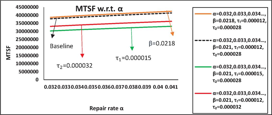
Figure 4 MTSF w.r.t. repair rate $\alpha$.

Figure 4 presents the system’s MTSF with respect to repair rate $\alpha$ (0.032–0.041) for different failure and repair rate parameters. The uppermost curve at repair rate $\beta =0.0218$, remainsconsistently above the base line curve $({\tau }_1=0.000012,{\tau }_2=0.000028,\beta =0.021)$, for all $\alpha$ values. Whereas the curves corresponding to increased failure rate ${\tau }_1$ and ${\tau }_2$ stays below than the base line curve, indicating that increasing failure rate declines the MTSF. However ${\tau }_2$ has a slightly stronger negative impact on MTSF than ${\tau }_1$.

Table 5 MTSF vs. Repair rate of system ${\mathrm{V}}_2$

Repair Rate	MTSF
$\beta$	$\begin{array}{c}{\tau }_1=0.000012\\ {\tau }_2=0.000028\\ \alpha =0.032\end{array}$	$\begin{array}{c}{\tau }_1=0.000012\\ {\tau }_2=0.000028\\ \alpha =0.033\end{array}$	$\begin{array}{c}{\tau }_1=0.000015\\ {\tau }_2=0.000028\\ \alpha =0.032\end{array}$	$\begin{array}{c}{\tau }_1=0.000012\\ {\tau }_2=0.000032\\ \alpha =0.032\end{array}$
0.021	37826419	38285202	30266568	14201887
0.0218	38681259	39161178	30950428	14522412
0.0226	39511067	40011964	31614263	14833555
0.0234	40316927	40838631	32258941	15135722
0.0242	41099860	41642191	32885279	15429295
0.025	41860832	42423599	33494049	15714636
0.0258	42600753	43183758	34085979	15992087
0.0266	43320486	43923524	34661760	16261969
0.0274	44020845	44643707	35222043	16524590
0.0282	44702601	45345074	35767445	16780238

MTSF: Table 5 examines the impact of changing one parameter on MTSF when it is calculated wth respect to repair rate $\beta$ of second system. For sensitive analysis all column values are compared to the base parameter set $({\tau }_1=\mathrm{\hspace{0.17em}0.000012},{\tau }_2=\mathrm{\hspace{0.17em}0.000028},\alpha =\mathrm{\hspace{0.17em}0.032})$. The most reliable configuration is the base column which displays the highest MTSF values. When $\alpha$ is increased from 0.032 to 0.033, the MTSF shows a consistent and average rise of 1.33%. This moderate improvement in MTSF proves $\alpha$, a mild positive sensitive parameter. When failure rate ${\tau }_1$ is increased from 0.000012 to 0.000015, the MTSF value decline by an average of approx. 19.99%. This pattern clearly identifies ${\tau }_1$ as the negatively sensitive parameter. The fourth column shows when ${\tau }_2$ is increase from 0.000028 to 0.000032, causing an average decrease of approx. 62.46%. Therefore, among all parameters, ${\tau }_2$ is the most negatively sensitive.

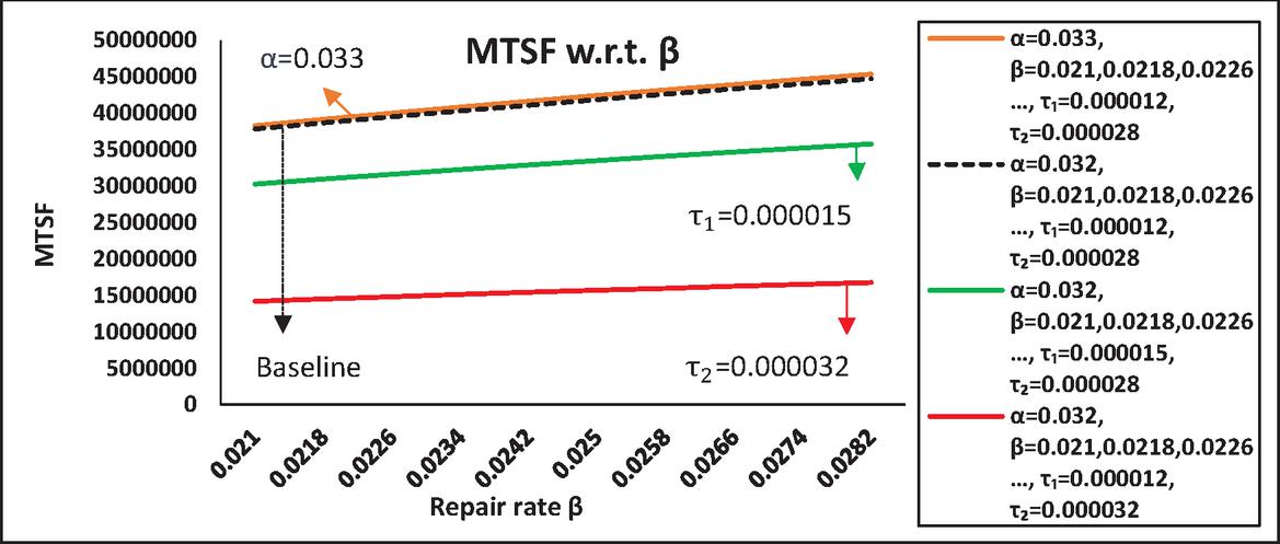
Figure 5 MTSF w.r.t. repair rate $\beta$.

Figure 5 shows the different trends of MTSF with respect to repair rate $\beta$ for different sets of failure and repair rate. The curve at ${\tau }_1=\mathrm{\hspace{0.17em}0.000015}$, is positioned lower than the base line curve $({\tau }_1=\mathrm{\hspace{0.17em}0.000012}$, ${\tau }_2=\mathrm{\hspace{0.17em}0.000028},\alpha =\mathrm{\hspace{0.17em}0.032})$, and the curve for ${\tau }_2=0.000032$ showing the steepest decline, indicating this parameter as the most negative sensitive for MTSF. The topmost curve for $\alpha =0.33$ is slightly above the baseline curve, suggesting MTSF increases monotonically as $\beta$ increases.

Table 6 Availability vs. Repair rate of system ${\mathrm{V}}_1$

Repair Rate	Availability
$\alpha$	$\begin{array}{c}{\tau }_1=0.000012\\ {\tau }_2=0.000028\\ \beta =0.021\end{array}$	$\begin{array}{c}{\tau }_1=0.000012\\ {\tau }_2=0.000028\\ \beta =0.0218\end{array}$	$\begin{array}{c}{\tau }_1=0.000015\\ {\tau }_2=0.000028\\ \beta =0.021\end{array}$	$\begin{array}{c}{\tau }_1=0.000012\\ {\tau }_2=0.000032\\ \beta =0.021\end{array}$
0.032	0.999999173	0.999999192	0.999998967	0.999999056
0.033	0.999999208	0.999999226	0.99999901	0.999999095
0.034	0.99999924	0.999999257	0.99999905	0.999999132
0.035	0.99999927	0.999999287	0.999999087	0.999999166
0.036	0.999999298	0.999999314	0.999999122	0.999999197
0.037	0.999999323	0.999999333	0.999999154	0.999999227
0.038	0.999999347	0.999999363	0.999999184	0.999999254
0.039	0.99999937	0.999999385	0.999999212	0.99999928
0.04	0.999999391	0.999999406	0.999999239	0.999999304
0.041	0.999999411	0.999999425	0.999999264	0.999999327

Availability: Table 6 presents the sensitive analysis of the availability when it is calculated with respect to repair rate $\alpha$ and examines the impact caused by change in single parameter. The first column is considered as the base column (with parameters ${\tau }_1=0.000012,{\tau }_2=$ $0.000028,\beta =0.021)$. As the repair rate $\alpha$ increases from 0.032 to 0.041 , availability gradually increases from 0.999999173 to 0.999999411 . In column 2 when $\beta$ is increased from 0.021 to 0.0218, a very moderate average increase of 0.000002% in availability is observed, indicating the least positive sensitivity. On the other hand, when ${\tau }_1$ is changed from 0.000012 to 0.000015, availability decreases by approximately 0.0000174%, confirming most negative sensitivity. Lastly, an increase in ${\tau }_2$ from 0.000028 to 0.000032 causes a decline in availability of around 0.000010%, proving ${\tau }_2$ to be the moderate negatively sensitive parameter affecting the system’s performance.

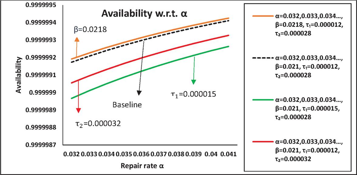
Figure 6 Availability w.r.t. repair rate $\alpha$.

Figure 6 shows how system’s availability behaves when calculated in reference to the repair rate $\alpha$ for different sets of repair and failure rates. The curve for $\beta =0.0218$ stays very closely but above than baseline curve $({\tau }_1=0.000012,{\tau }_2=0.000028,\beta =0.021)$, suggesting systems availability enhances with improved repair rate. Both the curves for ${\tau }_1=0.000015$ and ${\tau }_2=0.000032$ shift downward from the baseline curve, indicating ${\tau }_1$ leads more negative impact on system performance than ${\tau }_2$.

Table 7 Availability vs. Repair rate of system ${\mathrm{V}}_2$

Repair Rate	Availability
$\beta$	$\begin{array}{c}{\tau }_1=0.000012\\ {\tau }_2=0.000028\\ \alpha =0.032\end{array}$	$\begin{array}{c}{\tau }_1=0.000012\\ {\tau }_2=0.000028\\ \alpha =0.033\end{array}$	$\begin{array}{c}{\tau }_1=0.000015\\ {\tau }_2=0.000028\\ \alpha =0.032\end{array}$	$\begin{array}{c}{\tau }_1=0.000012\\ {\tau }_2=0.000032\\ \alpha =0.032\end{array}$
0.021	0.999999173	0.999999208	0.999998967	0.999997796
0.0218	0.999999192	0.999999226	0.99999899	0.999997845
0.0226	0.999999209	0.999999242	0.999999011	0.99999789
0.0234	0.999999224	0.999999258	0.999999031	0.999997933
0.0242	0.999999239	0.999999272	0.999999049	0.999997972
0.025	0.999999253	0.999999285	0.999999066	0.999998009
0.0258	0.999999266	0.999999298	0.999999083	0.999998043
0.0266	0.999999278	0.99999931	0.999999098	0.999998076
0.0274	0.99999929	0.999999321	0.999999112	0.999998107
0.0282	0.999999301	0.999999331	0.999999126	0.999998136

Availability: Table 7 quantify the sensitivity examination of system availability in reference to the repair rate $\beta$ of the second system. The first column, considered as the base column, shows that availability gradually increases as $\beta$ rises from 0.021 to 0.0282 . This base column is compared with the remaining columns, where one parameter is varied at a time while the others remain constant. An approximate average improvement of 0.000003% in system uptime exist when repair rate $\alpha$ is increased to 0.33, identifying $\alpha$ as the least positively sensitive parameter. Furthermore, availability consistently decreases, as the failure rates of both systems increase. The failure rate of first system, ${\tau }_1$ causes a very moderate negative sensitivity (approx. 0.000019%) in availability. Among the two failure rates, ${\tau }_2$ leads to an average decline of 0.000126%, making it the most negatively sensitive parameter in terms of impact on system performance.

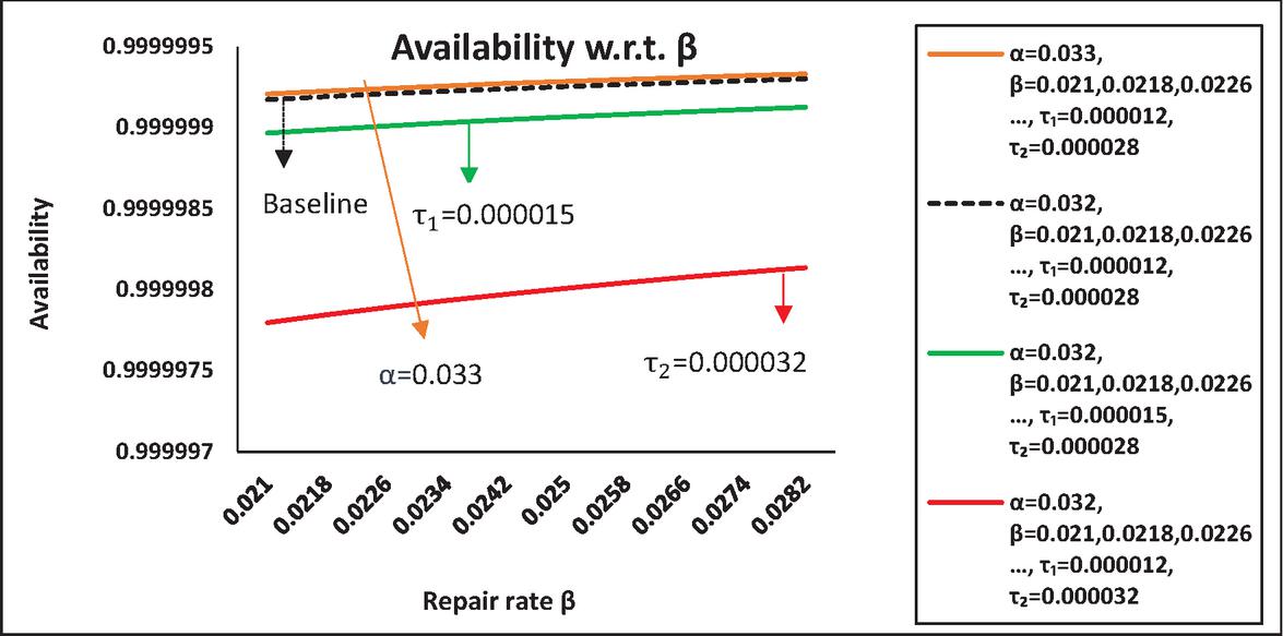
Figure 7 Availability w.r.t. repair rate $\beta$.

Figure 7 plots the availability with respect to repair rate $\beta$ (0.021–0.0282) for different parameter sets. The curve for increased repair rate, $\alpha =0.33$ shifts slightly upward than the baseline curve $({\tau }_1=0.000012,{\tau }_2=0.000028,\alpha =0.032)$. On the other hand, higher ${\tau }_2$ causing the steepest downward deviation in the curve than ${\tau }_1$.

Table 8 Profit vs. Repair rate of system ${\mathrm{V}}_1$

Repair Rate	Profit
$\alpha$	$\begin{array}{c}{\tau }_1=0.000012\\ {\tau }_2=0.000028\\ \beta =0.021\end{array}$	$\begin{array}{c}{\tau }_1=0.000012\\ {\tau }_2=0.000028\\ \beta =0.0218\end{array}$	$\begin{array}{c}{\tau }_1=0.000015\\ {\tau }_2=0.000028\\ \beta =0.021\end{array}$	$\begin{array}{c}{\tau }_1=0.000012\\ {\tau }_2=0.000032\\ \beta =0.021\end{array}$
0.032	79994.82019	79995.00702	79994.79027	79994.08922
0.033	79994.82286	79995.00966	79994.79362	79994.09228
0.034	79994.82534	79995.01209	79994.79671	79994.09512
0.035	79994.82763	79995.01435	79994.79957	79994.09774
0.036	79994.82975	79995.01644	79994.80223	79994.10018
0.037	79994.83173	79995.01838	79994.8047	79994.10245
0.038	79994.83358	79995.02019	79994.807	79994.10456
0.039	79994.8353	79995.02189	79994.80915	79994.10653
0.04	79994.83691	79995.02347	79994.81116	79994.10838
0.041	79994.83842	79995.02495	79994.81305	79994.11011

Profit: Table 8 assess the sensitive analysis of profit by considering first column as base column in which $\alpha$ is varying and for the set: ${\tau }_1=0.000012$, ${\tau }_2=0.000028,\beta =0.021$. When $\beta$ is increased from 0.021 to 0.0218 then profit is increased by 0.00097%. When failure rates ${\tau }_1$ and ${\tau }_2$ are raised then profit is decreased by the average value of 0.000034% and 0.000233% in third and fourth column respectively. This indicates that ${\tau }_2$ is the most sensitive (negative), ${\tau }_1$ is moderately sensitive (negative) parameter for profit.

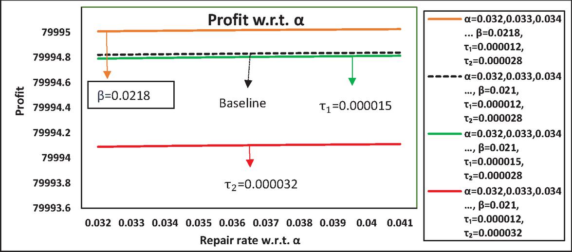
Figure 8 Profit w.r.t. repair rate $\alpha$.

The profit trends with respect to repair rate $\alpha (0.032-0.041)$ and at different parameter sets are displayed in Figure 8. The curve for $\beta =0.0218$ shows a gradual upward trend and lies above the baseline $({\tau }_1=0.000012,{\tau }_2=0.000028,\beta =0.021)$, showing that improving repair rate enhances system revenue. The curves corresponding to higher failure ${\tau }_1$ and ${\tau }_2$ as positioned below than the base curve, highlighting moderate and highest negative sensitivities, respectively.

Table 9 Profit vs. Repair rate of system ${\mathrm{V}}_2$

Repair Rate	Profit
$\beta$	$\begin{array}{c}{\tau }_1=0.000012\\ {\tau }_2=0.000028\\ \alpha =0.032\end{array}$	$\begin{array}{c}{\tau }_1=0.000012\\ {\tau }_2=0.000028\\ \alpha =0.033\end{array}$	$\begin{array}{c}{\tau }_1=0.000015\\ {\tau }_2=0.000028\\ \alpha =0.032\end{array}$	$\begin{array}{c}{\tau }_1=0.000012\\ {\tau }_2=0.000032\\ \alpha =0.032\end{array}$
0.021	79994.82019	79994.82286	79994.79027	79994.62084
0.0218	79995.00702	79995.00966	79994.97746	79994.81
0.0226	79995.18065	79995.18325	79995.15141	79994.98578
0.0234	79995.34242	79995.34498	79995.31348	79995.14955
0.0242	79995.4935	79995.49603	79995.46484	79995.30251
0.025	79995.63493	79995.63742	79995.60653	79995.44569
0.0258	79995.7676	79995.77006	79995.73945	79995.58
0.0266	79995.89229	79995.89473	79995.86437	79995.70624
0.0274	79996.00971	79996.01212	79995.98201	79995.82512
0.0282	79996.12048	79996.12286	79996.09298	79995.93726

Profit: In Table 9 profit is calculated with respect to repair rate $\beta$ and analysis the effect of changing one parameter on system revenue. In the second column, profit is increased by around 0.0000033%, claiming $\alpha$ as positively sensitive parameter. Increase in both failure rates ${\tau }_1$ and ${\tau }_2$, causes decline in profit, proving them negative sensitive parameter. The failure rate ${\tau }_1$ is moderately negatively sensitive with average decline of 0.000035% whereas ${\tau }_2$ leads to greater decline with an average 0.000239%.

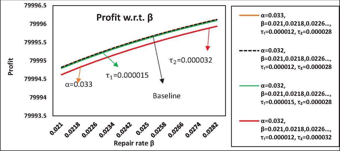
Figure 9 Profit w.r.t. repair rate $\beta$.

Figure 9 depicts how profit changes with respect to variations in repair rate $\beta$ for different combinations of failure rates $({\tau }_1,{\tau }_2)$ and repair rate $\alpha$. It can be observed that the curve for $\alpha =0.33$ is shifted slightly above from the baseline curve (${\tau }_1=0.000012,{\tau }_2=0.000028,\alpha =0.032)$. The steepest decline is observed for the curve at increased failure rate, ${\tau }_2=0.000032$. This indicates that increasing failure rate causing decline in revenue and hence this parameter leads a negative sensitivity on system revenue.

7 Conclusion

The analysis of the provided data on numerical representations of different reliability measures reveals several important findings and conclusions:

When the reliability metrics are evaluated with respect to the repair rate $\alpha$, the repair rate $\beta$ exhibits moderate positive sensitivity and the failure rates (${\tau }_1$ or ${\tau }_2$) are the negatively sensitive parameters affecting the system’s lifetime. Conversely, when the system reliability metrics are analysed with respect to the repair rate $\beta$, the failure rates (${\tau }_1$ or ${\tau }_2$) again emerge as the negatively sensitive parameters, $\alpha$ shows moderate sensitivity, and $\beta$ becomes the least sensitive parameter. As ${\tau }_1$ generally contributing significant reductions in uptime and revenue but to a lesser degree than ${\tau }_2$, suggesting ${\tau }_2$ the most negative sensitive parameter. In contrast, the sensitivity of $\alpha$ and $\beta$ is context-dependent. This suggests that, while improving repair mechanisms does enhance system performance, the most significant gains in reliability can be achieved by minimizing failure rates.

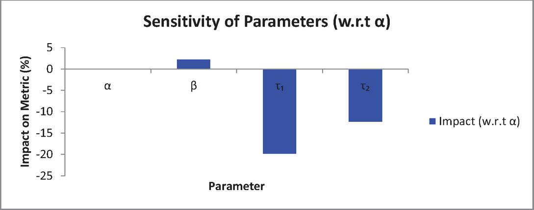
Figure 10 Sensitivity of parameters (w.r.t. $\alpha$).

Figure 10 depict the sensitive analysis (with respect to $\alpha$) as discussed in above conclusion. It demonstrates the positive bar height for $\beta$ suggests its moderate positive influence, while the deep negative bars for ${\tau }_1$ and ${\tau }_2$ illustrate their negative impact on system lifetime, with ${\tau }_1$ being the most negative.

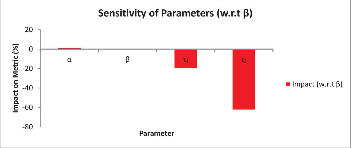
Figure 11 Sensitivity of parameters (w.r.t. $\beta$).

Figure 11 displays the sensitivity with respect to $\beta$, the positive effect of $\alpha$ is confirmed by the small positive bar. However the strong negative sensitivity for ${\tau }_1$ and especially ${\tau }_2$ can be observed by larger negative bars. This indicates that failure rate ${\tau }_2$ consistently exerts the most detrimental effect, while $\alpha$ and $\beta$ show positive influence whose magnitude depends on the reference parameter.

8 Limitations and Future Scopes

• The proposed model accounts only for corrective maintenance strategies where the repairs commencing only post-failures. The corrective-maintenance overlooks the industrial practices where the scheduled sustenance is essential. To overcome this certain proactive maintenance strategies can be adopted. Preventive maintenance conducts planned servicing or unit replacement at regular intervals to mitigate unforeseen failures. While condition-based maintenance performs continuous monitoring to avoid disrupt operation in advance. Hence future research can extend by employing preventive and condition-based techniques.

• Future studies may extend the model by incorporating non-exponential (Beta or Gamma) failure and repair time distribution under a semi-Markov environment to improve modeling realism and flexibility.

Data Availability Statement

We have no data to make available.

Conflict of Interest

The authors declare that they have no conflicts of interest.

References

[1] A. Al-Ammouri, V. Kharuta, A. Klochan, O. Shkurko, and H. Al-Ammori, Enhancing the Reliability of Information in Positioning Systems On Road Transport By Using Parallel Information Redundancy. Eastern-European Journal of Enterprise Technologies, 2024. DOI: 10.15587/1729-4061.2024.304129.

[2] A. K. Lado, and V. V. Singh. Cost assessment of complex repairable system consisting two subsystems in series configuration. International Journal of Quality and Reliability Management, 36(10): 1683–1699, 2019. DOI: 10.1108/IJQRM-12-2018-0322.

[3] A. Kumar. Parametric Optimization of Repairable Systems in IoT: Addressing Detection Delays, Imperfect Coverage, and Fuzzy Parameters, Life Cycle Reliability and Safety Engineering, 14: 329–340, DOI: 10.1007/s41872-025-00298-6.

[4] A. Kumar and M. Ram. Process modeling for decomposition unit of a UFP for reliability indices subject to fail-back mode and degradation, Journal of Quality in Maintenance Engineering, 29(3): 606–621, 2023, DOI: 10.1108/JQME-01-2022-0008.

[5] A. Kumar, D. Goyal, D. Sinwar, M. Saini. Stochastic modeling and performance optimization of sludge digestion processing system using genetic algorithm, International Journal of Information Technology, 14: 3391–3400, 2022. DOI: 10.1007/s41870-022-00908-x.

[6] A. Munjal, and S. B. Singh. Reliability analysis of a complex repairable system composed of a 2-out-of-3: G subsystem and a series subsystem connected in parallel. Journal of Reliability and Statistical Studies, 7: 19–39, 2014. DOI: 10.1007/s41872-019-00103-1.

[7] A. R. Kommula, and A. K. Mishra. Stochastic Reliability Modelling of Three-Component Systems under Simultaneous Failure Shocks. East Journal of Applied Science, 1–10, 2025. DOI: 10.63496/ejas.Vol1.Iss2.86.

[8] B. Singh, V. Saxena, R. Gupta, and S. Rathi. A Bayesian analysis of a geometric distribution model of two identical unit warm standby system with regular and expert repair facility. Reliability Assessment and Optimization of Complex Systems, 309–341, 2025. DOI: 10.1016/B978-0-443-29112-8.00018-9.

[9] C. Shekhar, S. Varshney, and A. Kumar. Standbys provisioning machine repair problem with unreliable service and vacation interruption, The Handbook of Reliability, Maintenance, and System Safety through Mathematical Modeling, A. Kumar and M. Ram, Eds. Elsevier, 101–137, 2021, DOI: 10.1016/B978-0-12-819582-6.00006-X.

[10] C. Wang, S. Luo, G. Chen, Z. Wu, W. Rong, and Q. Guan. Phase combination for reliability analysis of dynamic k-out-of-n Phase-AND mission systems. Reliability Engineering & System Safety, 257, 2025. DOI: 10.1016/j.ress.2025.110817.

[11] D. Kumar, D. Jana, S. Gupta, and P. Yadav. Bayesian Network Approach for Dragline Reliability Analysis: a Case Study. Mining Metallurgy & Exploration, 40(4), 2023. DOI: 10.1007/s42461-023-00729-x.

[12] D. Kumar, S. Gupta, and P. Yadav. Reliability, Availability, Maintainability of a Dragline, Journals of Mines, Metals and Fuels, 2020. DOI: 10.18311/jmmf/2020/26922.

[13] D. Mitra, S. B. Hamidi, P. Roy, C. Biswas, A. Biswas, and D. Dawn. Radio frequency reliability studies of CMOS RF integrated circuits for ultra-thin flexible packages, Electronic Letters, 56: 264–312, 2020. DOI: 10.1049/el.2019.3420.

[14] Gitanjali. Consistency of 2-out of -3 Redundant Systems with Priority of Repairing the Original Unit, International Journal of Agricultural and Statistical Sciences, 17(1): 2291–2299, 2021. DocID: https://connectjournals.com/03899.2021.17.2291.

[15] Gitanjali and S. C. Malik. Stochastic behaviour of the parallel system with expert repair and maintenance. Life Cycle Reliability and Safety Engineering, 8(1): 55–64, 2018. DOI: 10.1007/s41872-018-0064-6.

[16] J. R., Neyman, and E. L. Scott. Statistical Aspects of Queues, Operation Research, 6(1): 93–103, 1958.

[17] K. Ramesh and R. Gupta. Reliability of a Mechanical System with k-out-of-n subsystems. International Journal of Mechanical and Production Engineering Research and Development, 10(3): 7179–7188, 2020. DOI: 10.24247/IJMPERDJUN2020679.

[18] M. Todinov. Enhancing the Reliability of Series-Parallel Systems With Multiple Redundancies by Using System-Reliability Inequalities. Journal of Risk and Uncertainty in Engineering Systems, 9, 2024. DOI: 10.1115/1.4062892.

[19] Md. A. Lawan, U.A. Ali, A. L. Ismal, Md. S. Isa, A. S. Maihulla, and I. Yusuf. Reliability and Performance Analysis of Two Unit Active Parallel System Attended by Two Repairable Machines. International Journal of Operations Research, 19(2): 27–40, 2022. DOI: 10.6886/IJOR.202201_19(2).0001.

[20] M. Saini, D. Sinwar, A. M. Swarith, and A. Kumar. Reliability and maintainability optimization of load haul dump machines using genetic algorithm and particle swarm optimization. Journal of Quality in Maintenance Engineering, 29(2): 356–376, 2023. DOI: 10.1108/JQME-11-2021-0088.

[21] N. Jaiswal, S. Negi, and S. B. Singh. Reliability analysis of non-repairable weighted k-out-of-n system using belief universal generating function. International Journal of Industrial and Systems Engineering, 28: 300, 2018. DOI: 10.1504/IJISE.2018.089741.

[22] P. Baloda, A. Kumar, and V. Garg. Reliability Estimation of Parallel Systems with Diverse Failure Modes: Semi-Markov Model Approach. Journal of Reliability and Statistical Studies, 17, 2024. DOI: 10.13052/jrss0974-8024.1725.

[23] P. Kumar and A. Kumar. Time dependent performance analysis of a Smart Trash bin using state-based Markov model and Reliability approach, Cleaner Logistics and Supply Chain, 9, 2023, DOI: 10.1016/j.clscn.2023.100122.

[24] P. Lévy, Proceesus semi-markoviens, Proceedings of the International Congress of Mathematics, 3:416–426, 1954.

[25] P. M. Ferreira, J. Ou, C. Gaquière, and P. Benabes. Automated System-Level Design for Reliability: RF Front-End Application. Computational Intelligence in Analog and Mixed-Signal (AMS) and Radio-Frequency (RF) Circuit Design, 2015. DOI: 10.1007/978-3-319-19872-9_13.

[26] P. Sur, semi-Markov Processes, Theory of Probability & Its Applications, 6(1):21–38, 1961. DOI: 10.1137/1106003.

[27] R. Krishnan. Survey of Reliability Analysis of Weighted K-out-of-N System, Science Journal of Applied Mathematics and Statistics, 13: 15–21, 2025, DOI: 10.11648/j.sjams.20251301.12.

[28] R. Surapati, S. Akiri, S. R. Velampudi, and B. V. Nagarjuna. Enhancing Reliability of Series-Parallel Systems: A Novel Mathematical Model for Redundancy Allocation. European Journal of Pure and Applied Mathematic, 18(1):5672, 2025. DOI: 10.29020/nybg.ejpam.v18i1.5672.

[29] S. C. Malik and Gitanjali. A Parallel System with the Arrival time of Expert Server Subject to Maximum Repair and Inspection Times of Ordinary Server. Journal of Reliability and Statistical Studies, 7(1): 103–112, 2014.

[30] S. Jadhav, and A. Kumar. Stochastic modeling and availability optimization of wireless sensor network through particle swarm optimization. Reliability Engineering & System Safety, 265(B), 2026, DOI: 10.1016/j.ress.2025.111538.

[31] S. Kadyan, and S. C. Malik. Stochastic analysis of a three-unit non-identical repairable system with priority to main unit for operation and repair. International Journal of Quality & Reliability Management, 40(1), 2022, DOI: 10.1108/IJQRM-11-2020-0361.

[32] S. K. Kaul, and S. Dey. Reliability Analysis of RF MEMS Devices. Micromachined Circuits and Devices, 859: 225–245, 2022. DOI: 10.1007/978-981-16-9443-1_8.

[33] S. Kundu, A. Kumar and S. Varshney. Bayesian modeling of repairable systems with imperfect coverage and delayed detection dynamics. Quality and Reliability Engineering International, 41(4): 1630–1641, 2025, DOI: 10.1002/qre.3742.

[34] W. Feller. On the Integro-Differential Equations of Purely Discontinuous Markov Processes. Transactions of the American Mathematical Society, 48(3): 488–515, 1940.

[35] Y. Rani, I. Kumar, and Gitanjali. Reliability Modeling of Parallel Tubular and Plate Heat Exchangers using Regenerative Point Technique. International Journal of Information Technology, (2025). DOI: 10.1007/s41870-025-02636-4.

[36] Y. Rani, I. Kumar, and Gitanjali. Enhancing Sustainability through Reliability Optimization of Interconnected Pump and Water Supply Systems Using - a semi Markov Model. Scientific Reports, (2026). DOI: 10.1038/s41598-026-49337-x.

[37] Z. Li, H. Fu, and J. Guo, Reliability Assessment of a Series System with Weibull- Distributed Components Based on Zero-Failure Data. Applied Sciences, 15(5): 2869, 2025, DOI: 10.3390/app15052869.

Biographies

Yogita Rani is an accomplished Assistant Professor in the Department of Mathematics at Bhagwan Parshuram Institute of Technology, located in Rohini, Delhi. In addition to her teaching responsibilities, she is actively pursuing her research as a scholar at Manipal University, Jaipur. Her dual role as an educator and researcher reflects her commitment to advancing knowledge in the field of mathematics.

Gitanjali is a multifaceted academic professional, dedicated to the realm of reliability theory and modeling. With a specialization in Reliability Modeling, she has honed her expertise through 20 years of teaching in the Department of Applied Sciences at Maharaja Surajmal Institute of Technology, conducting research, and guiding aspiring scholars in this field. She employs statistical distributions as a powerful tool to meticulously analyze various repairable hardware devices. Her passion lies in the utilization of the semi-Markov process and the regeneration point technique to skillfully manage stochastic systems. She has also recognized for her extensive contributions to reputable journals through her research papers. She has also authored numerous mathematics textbooks and reference books, establishing herself as a respected figure in both academia and publishing.

Indeewar Kumar earned his Ph.D. in Boundary Layer Theory and Operations Research from VinobaBhave University, reflecting his deep expertise in these specialized areas. Currently, he serves as an Associate Professor in the Department of Mathematics and Statistics at Manipal University, Jaipur. With a distinguished academic career, Dr. Kumar has contributed significantly to his field through numerous research publications, particularly in the areas of operations research and boundary layer theory.

Journal of Reliability and Statistical Studies, Vol. 19, Issue 2 (2026), 555–586
doi: 10.13052/jrss0974-8024.19213
© 2026 River Publishers