A Quasi Poisson-Rama Distribution with Properties and Applications

Rama Shanker, Riki Tabassum and Jyotirmoyee Baishya^*

Department of Statistics, Assam University, Silchar, Assam, India
E-mail: shankerrama2009@gmail.com; rikitabassum18@gmail.com; jyotirmoyeebaishya790@gmail.com
*Corresponding Author

Received 03 November 2025; Accepted 16 April 2026

Abstract

A quasi Poisson-Rama distribution has been introduced which is the Poisson compound of quasi Rama distribution. The moments based descriptive properties have been discussed. The proposed distribution is unimodal, has increasing hazard rate and over-dispersed. The estimation of parameters has been studied using the method of moments and the method of maximum likelihood. A simulation study has been done to test the performance of maximum likelihood estimators of parameters. Finally, the goodness of fit of the proposed distribution has been discussed with two discrete datasets, the first from biological sciences and the second from thunderstorms and compared with the goodness of fit of Poisson-Lindley distribution, Poisson-Akash distribution, Poisson-Sujatha distribution, Poisson-Rama distribution, quasi Poisson-Lindley distribution, quasi Poisson-Akash distribution and quasi Poisson-Sujatha distribution.

Keywords: Quasi Rama distribution, compounding, mathematical and statistical properties, estimation of parameters, simulation, applications.

Abbreviations

PD	Poisson Distribution
NBD	Negative Binomial Distribution
PLD	Poisson-Lindley Distribution
PShD	Poisson-Shanker Distribution
PAD	Poisson-Akash Distribution
PSD	Poisson-Sujatha Distribution
RD	Rama Distribution
PDF	Probability Density Function
QRD	Quasi Rama Distribution
PRD	Poisson Rama Distribution
PMF	Probability Mass Function
QPRD	Quasi Poisson-Rama Distribution
QPLD	Quasi Poisson-Lindley Distribution
QPAD	Quasi Poisson-Akash Distribution
QPSD	Quasi Poisson-Sujatha Distribution
IHR	Increasing Hazard Rate
CV	Coefficient of Variation
CS	Coefficient of Skewness
CK	Coefficient of Kurtosis
ID	Index of Dispersion
CDF	Cumulative Distribution Function
MLE	Maximum Likelihood Estimator
MSE	Mean Square Error

1 Introduction

The PD is one of the primary discrete distributions for modeling equi-dispersed count data, where the mean equals the variance. In general, count data can be found in many areas of knowledge, such as biology, insurance, health, agriculture, engineering, etc. In real-world scenarios, it has been noted that the majority of stochastic datasets are either under-dispersed or over-dispersed. Numerous statistical methods, including weighted distributions and mixtures of distributions are suggested to address the over-dispersed count data. In recent decades, some researchers have attempted to create a one-parameter over-dispersed discrete distribution by compounding the PD with one parameter continuous lifetime distributions that are positively skewed. The chief characteristics of the Poisson mixture of positively skewed lifetime distribution is that the resultant distribution follows some characteristics of its mixing distribution.

During recent decades several over-dispersed count distributions have been introduced in statistics literature including NBD which is the PD compound of gamma distribution, PLD [1] which is the Poisson compound of Lindley distribution [2], PShD [3] which is the PD compound of Shanker distribution [4], PAD [5] which is the PD compound of Akash distribution [6] and PSD [7] which is the PD compound of Sujatha distribution [8]. A discrete quasi Akash distribution using discretization technique has been proposed by [9].

RD [10] is defined by its PDF

$$f(x;\theta )=\frac{{\theta }^4}{{\theta }^3+6}(1+x^3)e^{-\theta x};x>0,\theta >0.$$

Various statistical and reliability properties along with applications of RD have been discussed in [10]. A lot of works have been done in a short period of time on RD and its modifications. Two-parameter RD has been introduced where its properties and applications have also been discussed in [11]. The power version of RD and the weighted version of RD have been proposed by [12] and [13], respectively. Further extensions of RD include exponentiated RD by [14], extended RD by [15], new generalization of RD by [16], new variant of RD to model blood cancer data by [17], QRD by [18], wrapped Rama distribution by [19], some among others. A simple generalization of QRD has been proposed by [20].

Assuming the parameter $\lambda$ of the PD following RD, the PD compound of RD, named Poisson-Rama distribution (PRD) has been derived and studied by [21]. The PRD is defined by its pmf.

$P(X=x)={\displaystyle \frac{{\theta }^4}{{\theta }^3+6}}{\displaystyle \frac{x^3+6x^2+11x+({\theta }^3+3{\theta }^2+3\theta +7)}{{(\theta +1)}^{x+4}}};$

$x=0,1,2,\mathrm{\dots },\theta >0$

The descriptive properties based on moments, pmf and other statistical and reliability properties along with applications of PRD have been discussed in [21].

The QRD by [18] is defined by its PDF

$$f(x;\theta ,\alpha )=\frac{{\theta }^3}{\alpha {\theta }^2+6}(\alpha +\theta x^3)e^{-\theta x};x>0,\theta >0,\alpha >0$$

At $\alpha =\theta$, it reduces to RD. Descriptive statistical properties and applications of QRD are available in [18]. The weighted quasi Rama distribution (WQRD) and the power quasi Rama distribution (PQRD) have been proposed by [22] and [23], respectively.

The main motivation to propose QPRD which is the Poisson mixture of QRD is that it is highly flexible and applicable to over dispersed real-world count data. The interesting feature of QPRD is that it has the potential to handle a wide range of over-dispersed count data patterns and thus its versatility makes it useful for over-dispersed complex datasets commonly arising in the field of biomedical sciences and environmental studies. Although several Poisson mixture distributions are available in statistics literature but the main advantage of proposing QPRD for overdispersed data is that it allows the modeling of more extreme skewness than the standard one parameter PLD, PAD, PSD and PRD and two-parameter QPLD, QPAD and QPSD. The key difference between PRD and QPRD are that (i) PRD is of one parameter one parameter and QPRD is of two parameter and hence QPRD provides better fit in analysing real-world count datasets, where the over-dispersion is high often outperforming PRD in biological, medical and social sciences modeling. (ii) QPRD is a generalization of PRD and hence serves as a more flexible model for situations where PRD cannot sufficiently explain the variance in the dataset.

Various mathematical and statistical properties and estimation of parameters of QPRD have been discussed. Simulation study has been presented. The goodness of fit of QPRD has been compared with other one parameter and two-parameter distributions including PLD, PAD, PSD, PRD, QPLD [24], QPAD [25] and QPSD [26].

2 A Quasi Poisson-Rama Probability Model

Definition 1: The random variable $X$ is said to have QPRD if it follows the stochastic representation

$$X\mid \lambda \sim \mathrm{PD}(\lambda )\text{and}(\lambda \mid \theta ,\alpha )\sim \mathrm{QRD}(\theta ,\alpha )\text{for}\lambda >0,\theta >0,\alpha >0.$$

The unconditional distribution of the stochastic representation is denoted as $\mathrm{QPRD}(\theta ,\alpha )$.

Theorem 1: If $X\sim Q\mathrm{PRD}(\theta ,\alpha )$, then the PMF of $X$ is given by

$P(x;\theta ,\alpha )={\displaystyle \frac{{\theta }^3}{\alpha {\theta }^2+6}}{\displaystyle \frac{\theta (x^3+6x^2+11x+6)+\alpha {(\theta +1)}^3}{{(\theta +1)}^{x+4}}};$

$x=0,1,2,\mathrm{\dots },(\theta ,\alpha )>0$

Proof: If $X\mid \lambda \sim \mathrm{PD}(\lambda )$ and $\lambda \mid (\theta ,\alpha )\sim QRD(\theta ,\alpha )$, then the PMF of $X$ can be derived as

$$P(x;\theta ,\alpha )=P(X=x)={\int }_0^{\mathrm{\infty }}P(X=x\mid \lambda )f(\lambda \mid \theta ,\alpha )\mathit{d}\lambda$$

where $f(\lambda \mid \theta ,\alpha )$ is the QRD with parameter $\theta$ and $\alpha$.

We have

$P(x;\theta ,\alpha )$	$={\displaystyle {\int }_0^{\mathrm{\infty }}}{\displaystyle \frac{e^{-\lambda }{\lambda }^x}{x!}}{\displaystyle \frac{{\theta }^3}{\alpha {\theta }^2+6}}(\alpha +\theta {\lambda }^3)e^{-\theta \lambda }\mathit{d}\lambda$
	$={\displaystyle \frac{{\theta }^3}{(\alpha {\theta }^2+6)x!}}\left[\alpha {\displaystyle {\int }_0^{\mathrm{\infty }}}{e}^{-(\theta +1)\lambda }{\lambda }^x\mathit{d}\lambda +\theta {\displaystyle {\int }_0^{\mathrm{\infty }}}{e}^{-(\theta +1)\lambda }{\lambda }^{x+3}\mathit{d}\lambda \right]$	(1)
	$={\displaystyle \frac{{\theta }^3}{(\alpha {\theta }^2+6)x!}}\left[{\displaystyle \frac{\alpha \mathrm{\Gamma }(x+1)}{{(\theta +1)}^{x+1}}}+{\displaystyle \frac{\theta \mathrm{\Gamma }(x+4)}{{(\theta +1)}^{x+4}}}\right]$
	$={\displaystyle \frac{{\theta }^3}{\alpha {\theta }^2+6}}{\displaystyle \frac{\theta (x^3+6x^2+11x+6)+\alpha {(\theta +1)}^3}{{(\theta +1)}^{x+4}}};$
	$x=0,1,2,\mathrm{\dots },(\theta ,\alpha )>0$	(2)

Since this is the PD compound with QRD, we would call this probability model as QPRD. Also, at $\alpha =\theta ,\mathrm{QPRD}$ reduces to PRD. The PMF plot of QPRD for different values of parameters $\theta$ and $\alpha$ are presented in Figure 1.

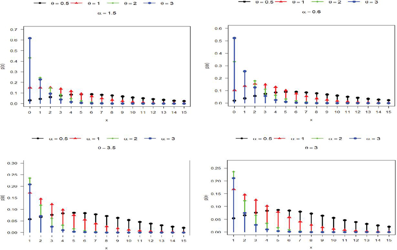
Figure 1 PMF of QPRD.

Theorem 2: The QPRD has IHR and is unimodal.

Proof: Since

$Q(x;\theta ,\alpha )$	$={\displaystyle \frac{P(x+1;\theta ,\alpha )}{P(x;\theta ,\alpha )}}$
	$={\displaystyle \frac{1}{\theta +1}}\left[1+{\displaystyle \frac{\theta (3x^2+15x+18)}{\theta (x^3+6x^2+11x+6)+\alpha {(\theta +1)}^3}}\right]$

is decreasing function of $x$ for a given $\theta$ and $\alpha ,P(x;\theta ,\alpha )$ is log-concave. Using the result about log-concave that log-concave functions are unimodal and has IHR from [27], we conclude that QPRD has an IHR and is unimodal.

Theorem 3: The $P(x;\theta ,\alpha )$ of QPRD is decreasing function of $x$ for given $\theta$ and $\alpha$.

Proof: We have

${\displaystyle \frac{P(x+1;\alpha ,\theta )}{P(x;\alpha ,\theta )}}={\displaystyle \frac{1}{\theta +1}}\left[1+{\displaystyle \frac{\theta (3x^2+15x+18)}{\theta (x^3+6x^2+11x+6)+\alpha {(\theta +1)}^3}}\right]$

$x=0,1,2,3,\mathrm{\dots }$

So for sufficiently large value of $x,\frac{P(x+1;\alpha ,\theta )}{P(x;\alpha ,\theta )}<1$. In fact from and after that stage for every $x$, we have $P(x+1;\alpha ,\theta )<P(x;\alpha ,\theta )$. Therefore, $P(x;\alpha ,\theta )$ is decreasing function of $x$ from and after a certain stage.

Theorem 4: The $\mathrm{pmf}P(x;\theta ,\alpha )$ of QPRD is log-concave and unimodel.

Proof: From [28, 29] and [30], a distribution having PMF $P(x;\theta )$ is log-concave if

$${[P(x+1;\theta )]}^2>P(x;\theta )\cdot P(x+2;\theta )\text{for}x\in N$$

(3)

Now for $\theta >0,\alpha >0$, it can be easily shown that the PMF given in (2)

$${[P(x+1;\theta )]}^2-P(x;\theta )\cdot P(x+2;\theta )>0\text{for all}x\in N.$$

Therefore, Equation (3) is satisfied for the pmf of QPRD given in (2). Again, using the results of [31] which states that log-concave pmf are strongly unimodal, the QPRD is also unimodal.

Theorem 5: The QPRD is a two-component mixture of NBD and can be expressed as

$$P(x;\theta ,\alpha )=p{P}_1(x;\theta )+(1-p)P_2(x;\theta ),$$

where $P_i(x;\theta )$ is the PMF of NBD with parameters the number of successes $i$ and $p=\frac{\alpha {\theta }^2}{\alpha {\theta }^2+6}$ with

$$P_1(x;\theta )=\frac{\theta }{{(\theta +1)}^{x+1}}\mathrm{as}NBD(1,\frac{\theta }{\theta +1})$$

and

$$P_2(x;\theta )=\frac{(x+1)(x+2)(x+3){\theta }^4}{6{(\theta +1)}^{x+4}}$$

as the NBD $(4,\frac{\theta }{\theta +1})$ respectively.

Proof: We have

$P(x;\theta ,\alpha )$	$={\displaystyle {\int }_0^{\mathrm{\infty }}}{\displaystyle \frac{e^{-\lambda }{\lambda }^x}{x!}}{\displaystyle \frac{{\theta }^3}{\alpha {\theta }^2+6}}(\alpha +\theta {\lambda }^3)e^{-\theta \lambda }\mathit{d}\lambda$
	$={\displaystyle {\int }_0^{\mathrm{\infty }}}{\displaystyle \frac{e^{-\lambda }{\lambda }^x}{x!}}\{{\displaystyle \frac{\alpha {\theta }^2}{\alpha {\theta }^2+6}}(\theta e^{-\theta \lambda })$
	$+{\displaystyle \frac{6}{\alpha {\theta }^2+6}}\left({\displaystyle \frac{{\theta }^4}{\mathrm{\Gamma }(4)}}{e}^{-\theta \lambda }{\lambda }^3\right)\}d\lambda$
	$={\displaystyle \frac{\alpha {\theta }^2}{\alpha {\theta }^2+6}}\left[{\displaystyle \frac{\theta }{x!}}{\displaystyle \frac{\mathrm{\Gamma }(x+1)}{{(\theta +1)}^{x+1}}}\right]$
	$+{\displaystyle \frac{6}{\alpha {\theta }^2+6}}\left[{\displaystyle \frac{{\theta }^4}{x!\mathrm{\Gamma }(4)}}{\displaystyle \frac{\mathrm{\Gamma }(x+4)}{{(\theta +1)}^{x+4}}}\right]$
	$={\displaystyle \frac{\alpha {\theta }^2}{\alpha {\theta }^2+6}}\left[NBD(1,{\displaystyle \frac{\theta }{\theta +1}})\right]+{\displaystyle \frac{6}{\alpha {\theta }^2+6}}\left[NBD(4,{\displaystyle \frac{\theta }{\theta +1}})\right]$
	$=p{P}_1(x;\theta )+(1-p)P_2(x;\theta )$

3 Moments Based Descriptive Statistics

Theorem 6: The $r$th factorial moment about origin ${\mu }_{(r)}^{\prime }$ of QPRD is given by

$${\mu }_{(r)}^{\prime }=\frac{r!\{\alpha {\theta }^2+(r+1)(r+2)(r+3)\}}{{\theta }^r(\alpha {\theta }^2+6)};r=1,2,3,\mathrm{\dots }$$

Proof: Using (2), ${\mu }_{(r)}^{\prime }$ can be obtained as

${\mu }_{(r)}^{\prime }$	$=E[E(X^{(r)}\mid \lambda )]$
	$={\displaystyle {\int }_0^{\mathrm{\infty }}}\left[{\displaystyle \sum _{x=0}^{\mathrm{\infty }}}{x}^{(r)}{\displaystyle \frac{e^{-\lambda }{\lambda }^x}{x!}}\right]{\displaystyle \frac{{\theta }^3}{\alpha {\theta }^2+6}}(\alpha +\theta {\lambda }^3)e^{-\theta \lambda }\mathit{d}\lambda$
	$={\displaystyle {\int }_0^{\mathrm{\infty }}}\left[{\lambda }^r{\displaystyle \sum _{x=r}^{\mathrm{\infty }}}{\displaystyle \frac{e^{-\lambda }{\lambda }^{x-r}}{(x-r)!}}\right]{\displaystyle \frac{{\theta }^3}{\alpha {\theta }^2+6}}(\alpha +\theta {\lambda }^3)e^{-\theta \lambda }\mathit{d}\lambda$
	$={\displaystyle \frac{r!\{\alpha {\theta }^2+(r+1)(r+2)(r+3)\}}{{\theta }^r(\alpha {\theta }^2+6)}};r=1,2,3,\mathrm{\dots }$

The first four factorial moments of QPRD is thus given by

${\mu }_{(1)}^{\prime }$	$={\displaystyle \frac{\alpha {\theta }^2+24}{\theta (\alpha {\theta }^2+6)}},{\mu }_{(2)}^{\prime }={\displaystyle \frac{2(\alpha {\theta }^2+60)}{{\theta }^2(\alpha {\theta }^2+6)}}$
${\mu }_{(3)}^{\prime }$	$={\displaystyle \frac{6(\alpha {\theta }^2+120)}{{\theta }^3(\alpha {\theta }^2+6)}},{\mu }_{(4)}^{\prime }={\displaystyle \frac{24(\alpha {\theta }^2+210)}{{\theta }^4(\alpha {\theta }^2+6)}}$

The first four moments about origin of the QPRD are given by

$${\mu }_1^{\prime }=\frac{\alpha {\theta }^2+24}{\theta (\alpha {\theta }^2+6)}$$

$${\mu }_2^{\prime }=\frac{\alpha {\theta }^3+2\alpha {\theta }^2+24\theta +120}{{\theta }^2(\alpha {\theta }^2+6)}$$

$${\mu }_3^{\prime }=\frac{\alpha {\theta }^4+6\alpha {\theta }^3+6\alpha {\theta }^2+24{\theta }^2+360\theta +720}{{\theta }^3(\alpha {\theta }^2+6)}$$

$${\mu }_4^{\prime }=\frac{\alpha {\theta }^5+14\alpha {\theta }^4+36\alpha {\theta }^3+24\alpha {\theta }^2+24{\theta }^3+840{\theta }^2+4320\theta +5040}{{\theta }^4(\alpha {\theta }^2+6)}$$

The moments about mean of QPRD can thus be obtained as

$${\mu }_2=\frac{{\alpha }^2{\theta }^5+{\alpha }^2{\theta }^4+30\alpha {\theta }^3+84\alpha {\theta }^2+144\theta +144}{{\theta }^2{(\alpha {\theta }^2+6)}^2}$$

$${\mu }_3=\frac{\left\{\begin{array}{c}{\alpha }^3{\theta }^8+3{\alpha }^3{\theta }^7+2{\alpha }^3{\theta }^6+36{\alpha }^2{\theta }^6+270{\alpha }^2{\theta }^5+396{\alpha }^2{\theta }^4\hfill \\ +\mathrm{\hspace{0.17em}324}\alpha {\theta }^4+1944\alpha {\theta }^3+648\alpha {\theta }^2+864{\theta }^2+2592\theta +1728\hfill \end{array}\right\}}{{\theta }^3{(\alpha {\theta }^2+6)}^3}$$

$${\mu }_4=\frac{\left\{\begin{array}{c}{\alpha }^4{\theta }^{11}+10{\alpha }^4{\theta }^{10}+18{\alpha }^4{\theta }^9+15{\alpha }^4{\theta }^8+42{\alpha }^3{\theta }^9+852{\alpha }^3{\theta }^8\hfill \\ +\mathrm{\hspace{0.17em}3132}{\alpha }^3{\theta }^7+3384{\alpha }^3{\theta }^6+540{\alpha }^2{\theta }^7+1180{\alpha }^2{\theta }^6\hfill \\ +\mathrm{\hspace{0.17em}34992}{\alpha }^2{\theta }^5+41472{\alpha }^2{\theta }^4+2808\alpha {\theta }^5+59184\alpha {\theta }^4\hfill \\ +\mathrm{\hspace{0.17em}132192}\alpha {\theta }^3+425088\alpha {\theta }^2+5184{\theta }^3+98496{\theta }^2+186624\theta \hfill \\ +\mathrm{\hspace{0.17em}2083968}\hfill \end{array}\right\}}{{\theta }^4{(\alpha {\theta }^2+6)}^4}$$

The descriptive constants based on moments namely CV, CS, CK and the ID of QPRD are given by

$$CV=\frac{\sqrt{{\mu }_2}}{{\mu }_1^{\prime }}=\frac{\sqrt{{\alpha }^2{\theta }^5+{\alpha }^2{\theta }^4+30\alpha {\theta }^3+84\alpha {\theta }^2+144\theta +144}}{\alpha {\theta }^2+24}$$

$$CS=\frac{{\mu }_3}{{\mu }_2^{3/2}}=\frac{\left\{\begin{array}{c}{\alpha }^3{\theta }^8+3{\alpha }^3{\theta }^7+2{\alpha }^3{\theta }^6+36{\alpha }^2{\theta }^6+270{\alpha }^2{\theta }^5\hfill \\ +\mathrm{\hspace{0.17em}396}{\alpha }^2{\theta }^4+324\alpha {\theta }^4+1944\alpha {\theta }^3+648\alpha {\theta }^2+864{\theta }^2\hfill \\ +\mathrm{\hspace{0.17em}2592}\theta +1728\hfill \end{array}\right\}}{{({\alpha }^2{\theta }^5+{\alpha }^2{\theta }^4+30\alpha {\theta }^3+84\alpha {\theta }^2+144\theta +144)}^{3/2}}$$

$$CK=\frac{{\mu }_4}{{\mu }_2^2}=\frac{\left\{\begin{array}{c}{\alpha }^4{\theta }^{11}+10{\alpha }^4{\theta }^{10}+18{\alpha }^4{\theta }^9+15{\alpha }^4{\theta }^8+42{\alpha }^3{\theta }^9\hfill \\ +\mathrm{\hspace{0.17em}852}{\alpha }^3{\theta }^8+3132{\alpha }^3{\theta }^7+3384{\alpha }^3{\theta }^6+540{\alpha }^2{\theta }^7\hfill \\ +\mathrm{\hspace{0.17em}1180}{\alpha }^2{\theta }^6+34992{\alpha }^2{\theta }^5+41472{\alpha }^2{\theta }^4+2808\alpha {\theta }^5\hfill \\ +\mathrm{\hspace{0.17em}59184}\alpha {\theta }^4+132192\alpha {\theta }^3+425088\alpha {\theta }^2+5184{\theta }^3\hfill \\ +\mathrm{\hspace{0.17em}98496}{\theta }^2+186624\theta +2083968\hfill \end{array}\right\}}{{({\alpha }^2{\theta }^5+{\alpha }^2{\theta }^4+30\alpha {\theta }^3+84\alpha {\theta }^2+144\theta +144)}^2}$$

$$ID=\frac{{\mu }_2}{{\mu }_1^{\prime }}=\frac{{\alpha }^2{\theta }^5+{\alpha }^2{\theta }^4+30\alpha {\theta }^3+84\alpha {\theta }^2+144\theta +144}{\theta (\alpha {\theta }^2+6)(\alpha {\theta }^2+24)}$$

Behaviour of CV, CS, CK and ID of QPRD for various values of parameters are shown in Figure 2.

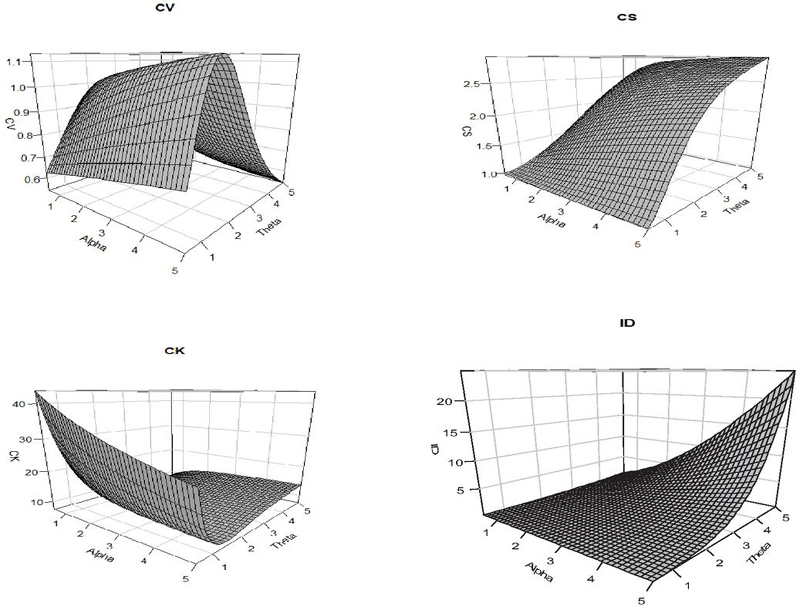
Figure 2 CV, CS, CK and ID of QPRD.

CV increases for increasing values of $\alpha$ and fixed $\theta$ while decreases for increasing values of $\theta$ and fixed $\alpha$. CS increases for increasing values of $\alpha$ and $\theta$ and the parameter $\alpha$ has more influence on CS than the parameter $\theta$. CK is highest when both the parameter $\alpha$ and $\theta$ is smaller which means that the distribution has heavier tails and sharper peaks in that region. As either parameter increases the kurtosis drops sharply that leads to a flatter and more uniform distribution. For higher values of the parameters $\alpha$ and $\theta$, ID increases which means that $\alpha$ and $\theta$ increases, the variance increases more than the mean, resulting into over-dispersion.

Theorem 7: The QPRD is over-dispersed, that is, ${\mu }_2>{\mu }_1^{\prime }$.

Proof: We have

${\mu }_2$	$={\displaystyle \frac{{\alpha }^2{\theta }^5+{\alpha }^2{\theta }^4+30\alpha {\theta }^3+84\alpha {\theta }^2+144\theta +144}{{\theta }^2{(\alpha {\theta }^2+6)}^2}}$
	$={\displaystyle \frac{\alpha {\theta }^2+24}{\theta (\alpha {\theta }^2+6)}}\left[{\displaystyle \frac{{\alpha }^2{\theta }^5+{\alpha }^2{\theta }^4+30\alpha {\theta }^3+84\alpha {\theta }^2+144\theta +144}{\theta (\alpha {\theta }^2+6)(\alpha {\theta }^2+24)}}\right]$
	$={\mu }_1^{\prime }\left[{\displaystyle \frac{({\alpha }^2{\theta }^5+30\alpha {\theta }^3+144\theta )+({\alpha }^2{\theta }^4+84\alpha {\theta }^2+144)}{{\alpha }^2{\theta }^5+30\alpha {\theta }^3+144\theta }}\right]$
	$={\mu }_1^{\prime }\left[1+{\displaystyle \frac{{\alpha }^2{\theta }^4+84\alpha {\theta }^2+144}{\theta (\alpha {\theta }^2+6)(\alpha {\theta }^2+24)}}\right].$

This gives ${\mu }_2>{\mu }_1^{\prime }$.

4 Reliability Properties

In this section, reliability properties of QPRD including survival function, hazard function, reverse hazard function and Mill’s ratio have been discussed.

The cdf of QPRD can be derived as

$F(x)$	$=F(x;\theta ,\alpha )=P(X\le x)=1-P(X\ge x+1)$
	$=1-{\displaystyle \sum _{t=x+1}^{\mathrm{\infty }}}{\displaystyle {\int }_0^{\mathrm{\infty }}}P(X=t\mid \lambda )f(\lambda ;\theta ,\alpha )\mathit{d}\lambda$
	$=1-{\displaystyle \sum _{t=x+1}^{\mathrm{\infty }}}{\displaystyle {\int }_0^{\mathrm{\infty }}}{\displaystyle \frac{e^{-\lambda }{\lambda }^t}{t!}}{\displaystyle \frac{{\theta }^3}{\alpha {\theta }^2+6}}(\alpha +\theta {\lambda }^3)e^{-\theta \lambda }\mathit{d}\lambda$
	$=1-{\displaystyle \sum _{t=x+1}^{\mathrm{\infty }}}{\displaystyle \frac{{\theta }^3}{(\alpha {\theta }^2+6)}}\left[{\displaystyle \frac{\alpha {(\theta +1)}^3+\theta (t+1)(t+2)(t+3)}{{(\theta +1)}^{t+4}}}\right]$
	$=1-{\displaystyle \frac{\left[\begin{array}{c}{\theta }^3{x}^3+(9{\theta }^3+3{\theta }^2)x^2+(26{\theta }^3+21{\theta }^2+6\theta )x]\hfill \\ +\left\{24{\theta }^3+36{\theta }^2+14\theta +\alpha {\theta }^2{(\theta +1)}^3\right\}\hfill \end{array}\right]}{(\alpha {\theta }^2+6){(\theta +1)}^{x+4}}}.$

The survival function of QPRD can thus be given by

$$S(x)=S(x;\theta ,\alpha )=\frac{\left[\begin{array}{c}{\theta }^3{x}^3+(9{\theta }^3+3{\theta }^2)x^2+(26{\theta }^3+21{\theta }^2+6\theta )x\hfill \\ +\{24{\theta }^3+36{\theta }^2+14\theta +\alpha {\theta }^2{(\theta +1)}^3\}\hfill \end{array}\right]}{(\alpha {\theta }^2+6){(\theta +1)}^{x+4}}.$$

The hazard function of QPRD can be expressed as

$h(x)$	$=h(x;\theta ,\alpha )$
	$={\displaystyle \frac{P(x;\theta ,\alpha )}{S(x;\theta ,\alpha )}}$
	$={\displaystyle \frac{{\theta }^4(x^3+6x^2+11x+6)+\alpha {\theta }^3{(\theta +1)}^3}{\left[\begin{array}{c}{\theta }^3{x}^3+(9{\theta }^3+3{\theta }^2)x^2\hfill \\ +(26{\theta }^3+21{\theta }^2+6\theta )x\hfill \\ +\{24{\theta }^3+36{\theta }^2+14\theta +\alpha {\theta }^2{(\theta +1)}^3\}\hfill \end{array}\right]}}$

The cdf, survival function and hazard function of QPRD shown in Figure 3. From the Graph of cdf of QPRD, it is clear that QPRD has a valid cdf because for $x\to \mathrm{\infty },F(x)\to 1$. Also, for fixed $\alpha ,{lim}_{x\to \mathrm{\infty }}h(x)=\theta$ and for fixed $\theta$, ${lim}_{x\to \mathrm{\infty }}h(x)=\alpha$.

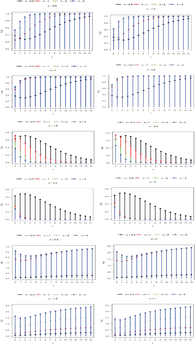
Figure 3 cdf, survival function and hazard function of QPRD.

The CDF shows how the probability builds up as the count variable increases. From the plots, it is clear that the cdf of QPRD increases smoothly with increasing $x$ and always remains between 0 and 1. This confirms that the proposed model is mathematically valid and suitable for count data. The parameter $\alpha$ affects how fast the cdf increases and $\theta$ affects the shape of the distribution.

The survival function decreases smoothly with increasing $x$. The parameter $\theta$ controls how quickly survival declines, while $\alpha$ affects the early behaviour of the curve. This shows that the distribution can model both rapid and slow decay in survival probabilities.

Hazard function represents the happening of an event at a particular value of $x$ given that the event has not occurred before. In the first graph of hazard function $\theta$ is fixed and $\alpha$ varies. In the 1st graph we have seen that as the value of alpha increases, initially the risk decreases then it increases steadily and after a certain point, it becomes almost constant. For smaller value of alpha, the risk increases in a very slow manner.

The second graph allows $\theta$ to vary and $\alpha$ to be fixed. In the 2nd graph we observed that the hazard function increases for all values of $\theta$. Initially there is a small decrease in risk for the highest value of $\alpha$. For smaller values of $\theta$, the risk remains low and increases gradually. As the value of $\theta$ increases, the hazard level becomes higher, but the overall pattern remains similar, this means that the rate of increase in risk is stable.

Reverse hazard function and Mill’s ratio of QPRD are obtained as

$\mathit{Rh}(x;\theta ,\alpha )$	$={\displaystyle \frac{P(x;\theta ,\alpha )}{F(x;\theta ,\alpha )}}$
	$={\displaystyle \frac{{\theta }^3\{\theta (x^3+6x^2+11x+6)+\alpha {(\theta +1)}^3\}}{\begin{array}{c}(\alpha {\theta }^2+6){(\theta +1)}^{x+4}\hfill \\ -[{\theta }^3{x}^3+(9{\theta }^3+3{\theta }^2)x^2+(26{\theta }^3+21{\theta }^2+6\theta )x\hfill \\ +\{24{\theta }^3+36{\theta }^2+14\theta +\alpha {\theta }^2{(\theta +1)}^3\}]\hfill \end{array}}}$

and

$M(x;\theta ,\alpha )$	$={\displaystyle \frac{S(x;\theta ,\alpha )}{P(x;\theta ,\alpha )}}$
	$={\displaystyle \frac{\begin{array}{c}[{\theta }^3{x}^3+(9{\theta }^3+3{\theta }^2)x^2+(26{\theta }^3+21{\theta }^2+6\theta )x\hfill \\ +\{24{\theta }^3+36{\theta }^2+14\theta +\alpha {\theta }^2{(\theta +1)}^3\}]\hfill \end{array}}{{\theta }^3\{\theta (x^3+6x^2+11x+6)+\alpha {(\theta +1)}^3\}}}$

5 Parameter Estimation

5.1 Method of Moment Estimation

Let $(x_1,x_2,\mathrm{\dots },x_n)$ be a random sample of size $n$ from the QPRD. We have

$$\frac{{\mu }_2^{\prime }-{\mu }_1^{\prime }}{{({\mu }_1^{\prime })}^2}=\frac{(2\alpha {\theta }^2+120)(\alpha {\theta }^2+6)}{{(\alpha {\theta }^2+24)}^2}=k$$

Taking $\alpha {\theta }^2=c$, we have

$$\frac{2(c+60)(c+6)}{{(c+24)}^2}=k$$

$$(k-2)c^2+(48k-132)c+576k-720=0$$

Replacing ${\mu }_1^{\prime }$ and ${\mu }_2^{\prime }$ with their corresponding sample moments, an estimate of $k$ can be obtained and substituting the value of $k$ in the above equation, estimate of $c$ can be obtained.

Now, for real root of $c$, we have

$${(48k-132)}^2-4(k-2)(576k-720)\ge 0\Rightarrow k\le 2.25$$

Thus, the method of moments estimate is applicable if $k=\frac{m_2^{\prime }-\overline{x}}{{(\overline{x})}^2}\le 2.25$, where $m_2^{\prime }$ and $\overline{x}$ are the corresponding second and first sample moments, respectively.

Now taking $\alpha {\theta }^2=c$ in the expression for mean and equating the population mean to the sample mean, we get the moment estimate $\tilde{\theta }$ of $\theta$ as

$$\frac{\alpha {\theta }^2+24}{\theta (\alpha {\theta }^2+6)}=\frac{c+24}{\theta (c+6)}=\overline{x}\Rightarrow \tilde{\theta }=\frac{c+24}{\overline{x}(c+6)}$$

From $\alpha {\theta }^2=c$, we get the moment estimate $\tilde{\alpha }$ of $\alpha$ as

$$\tilde{\alpha }=\frac{c}{{(\tilde{\theta })}^2}=\frac{c{(c+6)}^2{(\overline{x})}^2}{{(c+24)}^2}$$

Thus, the method of moment estimates $(\tilde{\theta },\tilde{\alpha })$ of $(\theta ,\alpha )$ of QPRD are given by

$$(\tilde{\theta },\tilde{\alpha })=(\frac{c+24}{\overline{x}(c+6)},\frac{c{(c+6)}^2{(\overline{x})}^2}{{(c+24)}^2})$$

5.2 Method of Maximum Likelihood Estimation

Suppose $(x_1,x_2,\mathrm{\dots },x_n)$ be a random sample from QPRD and let $f_x$ be the observed frequency corresponding to $X=x(x=1,2,3,\mathrm{\dots }k)$ such that ${\sum }_{x=1}^k{f}_x=n$, where $k$ is the largest observed value having non-zero frequency. The likelihood function, $L$ of the QPRD is given by

$L$	$={\left({\displaystyle \frac{{\theta }^3}{\alpha {\theta }^2+6}}\right)}^n$
	$\times {\displaystyle \frac{1}{{(\theta +1)}^{{\sum }_{x=1}^k(x+4)f_x}}}{\displaystyle \prod _{x=1}^k}[\theta (x^3+6x^2+11x+6)+\alpha {(\theta +1)}^3]$

The log-likelihood function is given by

$\log L$	$=n[3\log \theta -\log (\alpha {\theta }^2+6)]-{\displaystyle \sum _{x=1}^k}{f}_x(x+4)\log (\theta +1)$
	$+{\displaystyle \sum _{x=1}^k}{f}_x\log [\theta (x^3+6x^2+11x+6)+\alpha {(\theta +1)}^3]$

The maximum likelihood estimates $(\widehat{\theta },\widehat{\alpha })$ of $(\theta ,\alpha )$ are the solutions of equations

${\displaystyle \frac{\partial \log L}{\partial \theta }}$	$={\displaystyle \frac{3n}{\theta }}-{\displaystyle \frac{2n\alpha \theta }{\alpha {\theta }^2+6}}-{\displaystyle \frac{n(\overline{x}+4)}{\theta +1}}$
	$+{\displaystyle \sum _{x=1}^k}{\displaystyle \frac{(x^3+6x^2+11x+6)+3\alpha {(\theta +1)}^2}{\theta (x^3+6x^2+11x+6)+\alpha {(\theta +1)}^3}}=0$
${\displaystyle \frac{\partial \log L}{\partial \alpha }}$	$=-{\displaystyle \frac{n{\theta }^2}{\alpha {\theta }^2+6}}$
	$+{\displaystyle \sum _{x=1}^k}{\displaystyle \frac{{(\theta +1)}^3{f}_x}{\theta (x^3+6x^2+11x+6)+\alpha {(\theta +1)}^3}}=0$

where $\overline{x}$ is the sample mean. Since these two log-likelihood equations are not in closed form, it cannot be solved directly. But these equations can be solved using R-software.

6 A Simulation Study

In this simulation study, we evaluate the effectiveness of MLE for parameters $\theta$ and $\alpha$ of QPRD. The study considers multiple sample sizes (n $=$ 50, 100, 200, 300, 400, 500), with true values set at $\theta =3,\alpha =1$ and $\theta =3.5,\alpha =0.5$. The values of $\theta$ and $\alpha$ has been chosen on the basis of the estimates of the parameters for the proposed distribution. For simulating the sample, we used inverse transformation sampling. MLE is implemented using the stats4 package in R, applying the L-BFGS-B optimization method. For each sample size, 5,000 replications are used to compute performance metrics such as mean, variance, bias, and MSE. The results highlight improvements in estimation accuracy for increasing sample size and affirm the robustness of the MLE approach under this specific distributional setting.

$$\mathrm{bias}(\widehat{\theta })=E(\widehat{\theta })-\theta =\frac{1}{N}\sum _{i=1}^N{\widehat{\theta }}_i-\theta$$

$$\mathrm{MSE}(\widehat{\theta })=E\left[{(\widehat{\theta }-\theta )}^2\right]=\frac{1}{N}\sum _{i=1}^N{({\widehat{\theta }}_i-\theta )}^2$$

$$\mathrm{bias}(\widehat{\alpha })=E(\widehat{\alpha })-\alpha =\frac{1}{N}\sum _{i=1}^N{\widehat{\alpha }}_i-\alpha$$

$$\mathrm{MSE}(\widehat{\alpha })=E\left[{(\widehat{\alpha }-\alpha )}^2\right]=\frac{1}{N}\sum _{i=1}^N{({\widehat{\alpha }}_i-\alpha )}^2$$

Table 1 MSE and Bias for $\theta =3$ and $\alpha =1$

	$\theta =3$				$\alpha =1$
$N$	Mean	Variance	MSE	Bias	Mean	Variance	MSE	Bias
50	3.7184	1.5399	2.0559	0.7183	0.7835	0.3906	0.4374	$-0.2165$
100	3.4526	0.8414	1.0462	0.4526	0.8591	0.3401	0.3610	$-0.1409$
200	3.2886	0.4067	0.4838	0.3886	0.9104	0.2794	0.2874	$-0.0896$
300	3.1959	0.2626	0.3009	0.1959	0.9416	0.2480	0.2515	$-0.0584$
400	3.1454	0.1909	0.2182	0.1454	0.9621	0.2166	0.2025	$-0.0378$
500	3.1274	0.1659	0.1822	0.1273	0.9729	0.2018	0.2181	$-0.0271$

Table 2 MSE and Bias for $\theta =3.5$ and $\alpha =0.5$

	$\theta =3.5$				$\alpha =0.5$
$N$	Mean	Variance	MSE	Bias	Mean	Variance	MSE	Bias
50	4.0436	1.7796	2.0751	0.5436	0.6308	0.3742	0.3912	0.1308
100	3.8162	1.0729	1.1729	0.3162	0.6502	0.3263	0.3489	0.1523
200	3.6804	0.5922	0.6247	0.1804	0.6269	0.2531	0.2692	0.1269
300	3.6116	0.4122	0.4246	0.1116	0.6194	0.2175	0.2318	0.1194
400	3.5700	0.3223	0.3222	0.0700	0.6108	0.1841	0.1963	0.1108
500	3.5574	0.2632	0.2632	0.0574	0.5997	0.1592	0.1692	0.0997

From the Table 1 we observed that for the parameter $\theta$, the estimated mean moves closer to the true value $\theta =3$ as the sample size increases. At smaller sample sizes, the estimator shows more bias, but this bias steadily decreases with increasing sample size. Both the variance and the mean squared error (MSE) also decline sharply as the sample size increases, indicating improved precision and stability of the estimator. A similar trend is observed for the parameter $\alpha$. Same pattern has been seen in Table 2. For both table we can say that the estimators are consistent.

Table 3 Mammalian cytogenetic dosimetry lesions in rabbit lymphoblast induced by streptogramin

Number of Observations	Observed Frequency	Expected Frequency
				PLD	PAD	PSD	PRD	QPLD	QPAD	QPSD	QPRD
0	413	405.7	420.1	406.1	413.9	407.5	409.9	395.1	413.2
1	124	133.6	124.8	133.0	123.5	131.3	128.5	127.4	123.9
2	42	42.6	38.6	42.7	41.2	42.2	41.8	45.9	41.8
3	15	13.3	12.1	13.4	14.5	13.6	13.9	18.4	14.6
4	5	4.1	3.8	4.1	5.2	4.3	4.6	8.0	5.0
5	0	1.2	1.2	1.2	1.8	1.4	1.5	3.5	1.7
6	2	0.7	0.7	1.5	0.9	0.7	0.8	2.7	0.8
Total	601	601	601	601	601	601	601	601	601
$\widehat{\theta }(SE)$		2.6853 (0.1670)	3.0872 (0.1593)	3.1257 (0.1640)	3.1369 (0.1280)	2.2403 (0.4188)	2.6253 (1.0183)	2.4153 (0.7841)	3.4605 (1.3479)
$\alpha (SE)$						15.0060 (47.0648)	5.45822 (14.1681)	16.4112 (48.9510)	1.8442 (3.7322)
${\chi }^2$		4.8603	5.1153	1.1771	0.13929	0.68141	0.27049	5.512	0.0454
d.f.		3	3	3	3	2	2	2	2
p-value		0.5618	0.5291	0.8819	0.9977	0.9536	0.9916	0.2387	0.9997

Table 4 Number of thunderstorm events in the month of June

Number of Thunderstorms	Observed Frequency	Expected Frequency
				PLD	PAD	PSD	PRD	QPLD	QPAD	QPSD	QPRD
0	187	185.3	194.8	184.8	191.1	184.3	184.6	184.4	185.3
1	77	83.5	79.0	83.6	76.4	84.4	83.4	84.0	81.9
2	40	36.0	33.1	36.3	34.3	36.3	36.8	36.5	37.3
3	17	15.0	13.8	15.2	15.8	15.0	15.4	15.2	15.8
4	6	6.1	5.6	6.1	7.1	6.0	6.1	6.1	6.2
5	2	2.5	2.2	2.4	3.1	2.4	2.3	2.4	2.3
6	1	1.6	1.5	1.6	2.2	1.6	1.4	1.4	1.2
Total	330	330	330	330	330	330	330	330	330
$\widehat{\theta }(SE)$		1.8042 (0.1257)	2.2510 (0.1260)	2.2298 (0.1295)	2.4547 (0.1047)	1.8978 (0.4497)	2.5365 (0.5030)	2.2697 (0.4608)	3.2501 (0.5556)
$\widehat{\alpha }(SE)$						1.3459 (1.7615)	0.9516 (0.8563)	2.0299 (2.1131)	0.61325 (0.5117)
${\chi }^2$		1.3739	2.553	1.2573	2.0633	1.4322	1.0321	1.2506	0.6458
d.f.		3	3	3	3	2	2	2	2
p-value		0.8487	0.6352	0.8686	0.7241	0.8386	0.9049	0.8697	0.9578

7 Applications

In this section QPRD has been fitted on two real-life examples of observed count datasets and its goodness of fit has been compared with PLD, PAD, PSD, PRD, QPLD, QPAD and QPSD and presented in the Tables 3 and 4. The first dataset in Table 3 is related to mammalian cytogenetic dosimetry lesions in rabbit lymphoblast [32] and the second dataset is related to number of days that experienced the number of thunderstorms events at Cape Kennedy, Florida for the month of June, 11-year period of record January 1957 to December 1967 [33]. Based on the values of ${\chi }^2$, it is quite obvious that QPRD competes well with considered over-dispersed one parameter and two-parameter distributions and thus provides best fit among all considered distributions. In both datasets, QPRD yields smaller chi-square values and higher p-values among the considered distributions. Here, we would like to emphasize that algorithm for generating neutrosophic gamma distributed data by [34] and length-biased weighted Ishita distribution by [35] are popular for modeling continuous data but the Poisson mixture of these distributions is useful for modeling discrete data.

8 Conclusion

In this study, the PD compound of QRD named the QPRD has been proposed. It is specifically designed to model over-dispersed non-negative count data, particularly when the right tail of the data approaches zero quickly. Coefficients of variation, skewness, kurtosis, and index of dispersion are the measures based on moments have been derived and their behaviour for different parameter values has been studied. The QPRD is shown to be overdispersed, unimodal, has an increasing hazard rate and right-skewed. It is a two-component mixture of NBDs, yet it maintains its unimodality in its PMF which suggest that modes of its constituent sub-populations are located very close to each other. The estimation of parameters of QPRD has been discussed with both the method of moments and the method of maximum likelihood. The effectiveness of maximum probability estimates has been tested using simulation. The goodness of fit of QPRD has been tested with two datasets and compared with the goodness of fit of PLD, PAD, PSD, PRD, QPLD, QPAD and QPSD. It is clear that QPRD is the best distribution among all one parameter and two-parameter over-dispersed discrete distributions and therefore, QPRD would be the best probability model for over-dispersed count data in data science. It is quite clear that QPRD is particularly suited for biological sciences, insurance and other fields characterized by heavily over-dispersed count data.

The QPRD has some limitations. Since the proposed distribution has only two-parameter which may limits its flexibility compared to three-parameter or more complex models when dealing with extremely diverse datasets. It is designed for over-dispersed dataset and is not suitable for under-dispersed dataset. Although the proposed distribution is flexible, its unimodal nature means that it cannot be used to model multi-modal data structures.

As the distribution is new and thus have high potential for applications in different fields of knowledge and we are sure that in future the proposed distribution will draw attention of researchers in biomedical sciences and engineering to model survival time data. The future research possibilities are that size-biased and zero-truncated versions of QPRD can be derived and their applications for the data excluding zero counts can be examined. Some more areas of applications in other fields of knowledge can be explored for big data in the data science. For example, zero-inflated Poisson quasi Rama distribution can be developed to model data with excessive zeros. The QPRD can be extended into a regression framework named Poisson quasi Rama regression to examine the relationship between the dependent variable and covariates. The proposed distribution can be modified to handle under-dispersed data.

Acknowledgements

Authors are grateful to the editor in chief and the two anonymous reviewers for their fruitful comments which improved both the quality and presentation of the paper.

References

[1] Sankaran, M. The discrete Poisson-Lindley distribution, Biometrics, 26(1): 145–149, 1970.

[2] Lindley, D. V. Fiducial distributions and Bayes theorem, Journal of Royal Statistical Society, 20(1): 102–107, 1958.

[3] Shanker, R. The discrete Poisson-Shanker distribution, Jacobs Journal of Biostatics, 1(1): 1–7, 2016.

[4] Shanker, R. Shanker distribution and its applications, International Journal of Statistics and Applications, 5(6): 338–348, 2015.

[5] Shanker, R. The discrete Poisson-Akash distribution, International Journal of Probability and Statistics, 6(1): 1–10, 2017.

[6] Shanker, R. Akash distribution and its applications, International Journal of Probability and Statistics, 4(3): 65–75, 2015.

[7] Shanker, R. The discrete Poisson-Sujatha distribution, International Journal of Probability and Statistics, 5(1): 1–9, 2016.

[8] Shanker, R. Sujatha distribution and its applications, Statistics in Transition-New Series, 17(3): 391–410, 2016.

[9] Abebe, B., and Shanker, R. A discrete quasi Akash distribution with applications, Turkiye Klinikleri Journal of Biostatistics, 10(3): 187–199, 2018.

[10] Shanker, R. Rama distribution and its application, International Journal of Statistics and Applications, 7(1): 26–35, 2017.

[11] Edith, U. U., Ebele, T. U., and Henrietta, A. I. A two-parameter Rama distribution, Earthline Journal of Mathematical Sciences, 2(2): 365–382, 2019.

[12] Abebe, B., Tesfay, M., Eyob, T., and Shanker, R. A two-parameter power Rama distribution with properties and applications, Biometrics & Biostatistics International Journal, 8(1): 6–11, 2019.

[13] Eyob, T., and Shanker, R. A two-parameter weighted Rama distribution with properties and application, Universal Journal of Mathematics and Applications, 2(2): 48–58, 2019.

[14] Onyekwere, C. K., Osuji, G. A., Enogwe, S. U., Okoro, M. C., and Ihedioha, V. N. Exponentiated Rama Distribution: properties and application, Mathematical theory and Modelling, 11(1): 2224–5804, 2021.

[15] Alhyasat, K. M., Ibrahim, K., Al-Omari, A. I., and Bakar, M. A. A. Extended Rama distribution: properties and applications, Computer System Science Engineering, 39(1): 55–67, 2021.

[16] Mohiuddin, M., and Kannan, R. A new generalization of Rama distribution with application to machinery data, International Journal of Emerging Technologies in Engineering Research, 9(9): 1–13, 2021.

[17] Omoruyi, F. A., Omeje, I. L., Anabike, I. C., and Obulezi, O. J. A new variant of Rama distribution with simulation study and application to blood cancer data, European Journal of Theoretical and Applied Sciences, 1(4): 389–409, 2023.

[18] Shanker, R., Das, H., and Shukla, K. K. A quasi Rama distribution, Model Assisted Statistics and Applications, 18(3): 267–277, 2023.

[19] Bell, W., and Nadarajah, S. The wrapped Rama distribution, Scientific Reports, 14(1): 31936, 2024.

[20] Arunachalam, R. A new generalisation of the quasi Rama distribution: Exploring its Statistical Properties and Applications, Mathematics and Computer Science: Research Updates, 4: 64–83, 2025.

[21] Shanker, R., Ray, M., and Shukla, K. K. The Poisson-Rama distribution with properties and applications to model over-dispersed count data, Brazilian Journal of Biometrics, 43(2): 1–15, 2025.

[22] Shanker, R., Ray, M., Prodhani, H. R., and Boruah, J. Weighted quasi Rama distribution with properties and applications in Engineering, International Journal of Statistics and Reliability Engineering, 12(1): 18–34, 2025.

[23] Shanker, R., Prodhani, H. R., Ray, M., and Deb, J. Power quasi Rama distribution with properties and applications in reliability engineering, Journal of Probability and Statistical Science, 24(1): 50–73, 2026.

[24] Shanker, R., and Mishra, A. A quasi Poisson-Lindley distribution, Journal of Indian Statistical Association, 54(1&2): 113–125, 2016.

[25] Shanker, R., Shukla, K. K., and Shanker, R. A quasi Poisson-Akash distribution and its applications to ecology, International Journal of Statistics and Applied Mathematics, 3(3): 111–119, 2018.

[26] Shanker, R., and Shukla, K. K. A quasi Poisson-Sujatha distribution with applications, Journal of Applied Probability and Statistics, 14(1): 103–115, 2019.

[27] Grandell, J. Mixed Poisson Processes, Chapman & Hall, London, 1997.

[28] Gupta, P. L., Gupta, R. C., Tripathi, R. C. On the monotonic properties of discrete failure rates, Journal of statistical planning and inference, 65(2): 255–268, 1997.

[29] Steutal, F. Log-concave and log-convex distribution, Encyclopedia of Statistical Sciences, 2004.

[30] Bagnoli, M., Bergstrom, T. Log-concave probability and its application in Rationality and Equilibrium: A symposium is Honoured of Marchel K. Richer, Springer, 217–241, 2006.

[31] Keilson, J., Gerber, H. Some results for discrete unimodality, Journal of the American Statistical Association, 66(334): 386–389, 1971.

[32] Pittillo, R. F., and Woolley, C. Biological assay of streptonigrin (NSC 45383) in body fluids and tissues of mice, Antimicrobial agents and chemotherapy, 5(1): 82–85, 1974.

[33] Falls, L. W., Williford, W. O., and Carter, M. C. Probability distributions for thunderstorm activity at Cape Kennedy, Florida, Journal of Applied Meteorology, 10(1): 97–104, 1971.

[34] Saleem, M., and Aslam, M. Algorithms for Generating Neutrosophic Gamma Distributed Data, Journal of Reliability and Statistical Studies, 2025.

[35] Pushkarna, N., and Mustafa, M. Length Biased Weighted Ishita Distribution and Its Applications on Real Life Data Sets, Journal of Reliability and Statistical Studies, 2025.

Biographies

Rama Shanker received his Ph.D. Degree in Statistics from Patna University, Patna, India. He is currently working as Professor of Statistics in the Department of Statistics, Assam University, Silchar, Assam, India. He Has 235 research papers in his name in reputed Journals of Statistics, Mathematics, Operations Research and Biostatistics. He has 22 years of post-Ph.D teaching and research experience at undergraduate and postgraduate level. He has successfully guided four Ph.D. Scholars and currently five research scholars are working under his supervision for Ph.D. degree.

Riki Tabassum obtained her master Degree in Statistics from Guwahati University, Guwahati, India. She is currently a research scholar in the Department of Statistics, Assam University, Silchar and working for her Ph.D. Degree in Distribution Theory. She has published seven research papers in reputed Journals of Statistics. She has also presented three research papers in international conferences.

Jyotirmoyee Baishya obtained her master Degree in Statistics from Assam University, Silchar, India. She is currently a research scholar in the Department of Statistics, Assam University, Silchar and working for her Ph.D. Degree in Distribution Theory. She has published six research papers in reputed Journals of Statistics. She has also presented two research papers in international conferences.

Journal of Reliability and Statistical Studies, Vol. 19, Issue 2 (2026), 285–310.
doi: 10.13052/jrss0974-8024.1923
© 2026 River Publishers