Improving Finite Population Mean through Ranked Sets

Poonam Singh¹, Sooraj Gupta^1,*, Pooja Maurya¹ and Prayas Sharma²

¹Department of Statistics, Banaras Hindu University, Varanasi – 221005, India
²Department of Statistics, Babasaheb Bhimrao Ambedkar University, Lucknow, India
E-mail: poonamsingh@bhu.ac.in; soorajgpt@bhu.ac.in; poojamaurya@bhu.ac.in; prayassharma02@gmail.com
*Corresponding Author

Received 15 January 2026; Accepted 19 May 2026

Abstract

In the field of sampling theory, simple random sampling (SRS) has been widely used and proven to be effective for drawing samples to estimate population parameters. However, in certain situations, obtaining observations on the study variable is more challenging than ranking the units. In such cases, ranked set sampling (RSS) becomes very useful in the estimation of population parameters. We offer two new estimators under RSS to estimate the finite population mean out of which one estimator is equivalent to the many estimators existing in the literature, Therefore it can be used as the alternatives to the existing ones while the other one performs better than the recent estimator Khalid et al., (2024) in terms of mean squared error (MSE) and percentage relative efficiency (PRE), under RSS framework. Among the two proposed estimators, One of these estimators combines log and exponential, while the other combines regression and exponential.We found that second estimator turns out to be most efficient among the estimators studied in this study under RSS. The MSE and PRE are employed to evaluate the performance of the proposed estimators in comparison with traditional estimators discussed in this study. Analytical expressions for the MSE and bias are derived, along with the conditions under the proposed estimators demonstrate improved efficiency. To substantiate the theoretical findings, both empirical and simulation studies are conducted. The results indicate that the proposed estimators provide better performance compared to traditional estimators.

Keywords: Ratio-type exponential estimator, Ranked set sampling (RSS), Log-type exponential estimator, Bias, Mean-squared error (MSE), Percentage relative efficiency (PRE), Simulations.

1 Introduction

The systematic use of auxiliary information in mean estimation was first formalized by Cochran, (1940), who demonstrated that incorporating an auxiliary variable $X$ correlated with the study variable $Y$ can substantially improve estimation efficiency. Since then, auxiliary variables have been recognized not merely as convenient supplements, but as carriers of structural population information that can be strategically exploited at both the design and estimation stages. In many practical surveys, while direct observation of $Y$ is costly or restrictive, auxiliary characteristics are readily available and reveal ordering, proportionality, or variability patterns within the population. When effectively utilized, such information enhances precision without increasing sample size, thereby strengthening inference through informed use of population-level relationships. A substantial body of literature has emerged on estimation techniques based on auxiliary information; interested readers may consult these recent contributions for further developments such as Singh et al., (2024), Kumari et al., (2025), Sharma et al., (2025) and Singh and Singh, (2026).

In survey sampling practice, situations often arise where obtaining observations on the study variable, or the variable of interest, is either highly difficult or in some cases not feasible at all. However, ranking the units is usually much more convenient and can be accomplished through judgmental ordering or other ranking methods, which typically involve minimal or no additional cost. It is very established fact that estimate of population mean under RSS is more efficient than under simple random sampling (Halls and Dell, (1966), Muttlak and McDonald, (1992)). McIntyre, (1952), pioneered the concept of RSS without building its mathematical concepts. He used RSS to estimate the pasture yield through more represented observations. Takahasi and Wakimoto, (1968) attempted to provide its mathematical theory. They concluded that sample mean under RSS is more efficient than the same under SRS of the same sample size. Dell and Clutter, (1972), analyzed the RSS method under the assumption that ranking is not perfect. Their study demonstrated that RSS is more efficient than SRS of the same size regardless of whether the ranking is perfect or imperfect. For a clearer and more comprehensive understanding of RSS, researchers may also refer to the works of Jafari Jozani and Johnson, (2011) and Wolfe, (2012).

Lynne Stokes, (1977) was the first to address situations where it is difficult to order the observations based on the study characteristic. She suggested that such ordering can be achieved by ranking the observations with respect to an auxiliary characteristic. Recognizing the potential of RSS in providing a more representative sample compared to SRS, it is now increasingly applied in diverse areas such as statistical process control for developing efficient control charts (Woodall et al., (2024)), demographic studies (Kumari et al., (2024)), field of energy(Vishwakarma and Singh, (2022)) and many more. With the growing applicability of RSS, driven by the pursuit of more representative samples, several new modifications of RSS have been proposed, such as median ranked set sampling (Zarinkolah et al., (2024)), Double extreme-cum-median ranked set sampling (Zubair et al., (2024)), etc.

In the row of development of new and efficient estimators to estimate the mean of a finite population, Samawi and Muttlak, (1996) were the first to incorporate auxiliary variable for proposing a ratio estimator under ranked set sampling. Philip and Lam, (1997) proposed regression estimator under RSS. Then authors such as Kadilar et al., (2009) proposed a general form of the estimator proposed by Samawi and Muttlak, (1996) to estimate the mean of a finite population under RSS. To provide more efficient estimator under RSS, Vishwakarma et al., (2017) proposed an exponential type estimator under RSS. Mehta et al., (2020) proposed a general class of estimators employing the linear combination of two estimators. To further study the development of such efficient estimators under RSS, we can consider the original articles including Khalid et al., (2022), Bhushan and Kumar, (2022),Bhushan et al., (2022), Khalid et al., (2024). Kumari et al., (2024), Vishwakarma and Singh, (2022) and Bhushan et al., (2023) documented some updated class of estimators to estimate mean of the finite population under RSS. Many authors have proved that logarithmic estimators show better efficiency while dealing with non-linear population. Over times several estimators have been proposed in this direction for the estimation of finite population population parameters. Zaman and Iftikhar,(2023) proposed a logarithmic ratio-type estimator under simple random sampling scheme. Zaman et al.,(2024) proposed a new logarithmic type estimator to analyse the number of aftershocks. More recently, Singh et al.,(2025), proposed a log-transformed approach to estimate the population variance. For more information in this direction, researchers may refer to Audu et al.,(2025), Shukla et al.,(2026) and Djebar et al.,(2026).

The pursuit of more efficient estimators in survey sampling continues to be a fundamental objective in statistical research. Motivated by this ongoing need, the present study proposes two novel estimators under RSS for estimating the finite population mean. The first proposed estimator performs comparably to the generalized estimator introduced by Khalid et al., (2024), while the second demonstrates improved efficiency relative to this recent contribution within the RSS framework. The first estimator is formulated as a nonlinear combination of two fundamental components. In contrast, the second estimator is constructed as a linear combination of the same components, thereby yielding a more general and flexible class of estimators.

The remainder of the manuscript is organized as follows. Section 2 reviews existing methodologies for estimating the finite population mean. Section 3 presents the theoretical development of the proposed estimators and derives expressions for their bias and MSE up to the first order of approximation. Section 4 provides a comprehensive comparison study, establishing the conditions under which the proposed estimators outperform the traditional ones. To validate the theoretical findings, Section 5 presents a numerical investigation, including both empirical and simulation studies. Finally, Section 6 offers a detailed discussion and conclusion summarizing our findings.

1.1 Notations

Let us suppose that we have a finite population of size N. To estimate the population mean of a study characteristic (Y) with help of a auxiliary variable (X) the following procedure under RSS have been followed to take a sample of size n.

Procedure for taking a sample using RSS:

1. Take $m$ random sample of size m from a population.

2. Rank the random sample of size $m$ using any cost-effective method, such as visual (eye) observation or other available auxiliary information.

3. Take smallest ranked unit from the first random sample, second smallest ranked unit from the second random sample and similar procedure is followed till we get the largest ranked unit. Eventually, we get $m$ ordered units.

4. To take a sample of size $n$ ($=mr$) under RSS, we repeat the above steps r times.

5. At the final stage, we collect information on those units of the study variable which have been selected under this procedure.

$m:\text{Total number of ordered observations selected under}$

$\text{particular replication},$

$r:\text{Total numbers of replications for taking a ranked set sample of size n},$

$n=mr:\text{Sample size},$

$N:\text{Population size},$

$\overline{Y}={\displaystyle \frac{1}{N}}{\displaystyle \sum _1^N}{Y}_i:\text{Population mean of the study variable},$

$\overline{X}={\displaystyle \frac{1}{N}}{\displaystyle \sum _1^N}{X}_i:\text{Population mean of the auxiliary variable}$

${\overline{y}}_{[n]}={\displaystyle \frac{1}{mr}}{\displaystyle \sum _{i=1}^m}{\displaystyle \sum _{j=1}^r}{y}_{[i]j}:\text{Sample mean of the study variable based on}$

the ranked set sample of size mr

${\overline{x}}_{(n)}={\displaystyle \frac{1}{mr}}{\displaystyle \sum _{i=1}^m}{\displaystyle \sum _{j=1}^r}{x}_{(i)j}:\text{Sample mean of the auxiliary variable based on}$

$\text{the ranked set sample of size}mr,$

${\mu }_{[y]}(i)={\displaystyle \frac{1}{r}}{\displaystyle \sum _{j=1}^r}{y}_{[i]j}:\text{Sample mean of the}{i}^{th}\text{ranked units selected in the}$

$\text{sample of size}mr\text{under study variable},$

${\mu }_{(x)}(i)={\displaystyle \frac{1}{r}}{\displaystyle \sum _{j=1}^r}{x}_{(i)j}:\text{Sample mean of the}{i}^{th}\text{ranked units selected in the}$

$\text{sample of size}mr\text{under auxiliary variable},$

$C_Y={\displaystyle \frac{\sqrt{{\displaystyle \frac{1}{N}}{\sum }_{i=1}^N{(Y_i-\overline{Y})}^2}}{\overline{Y}}}:\text{Population coefficient of variation of the}$

$\text{study variable},$

$C_X={\displaystyle \frac{\sqrt{{\displaystyle \frac{1}{N}}{\sum }_{i=1}^N{(X_i-\overline{X})}^2}}{\overline{X}}}:\text{Population coefficient of variation of the}$

$\text{auxiliary variable},$

$C_{YX}={\displaystyle \frac{\sqrt{{\displaystyle \frac{1}{N}}{\sum }_{i=1}^N(Y_i-\overline{X})(X_i-\overline{X})}}{\overline{Y}\overline{X}}},$

$A_{y[i]}^2={\displaystyle \frac{1}{m^{2}r{\overline{y}}_{[n]}^2}}{\displaystyle \sum _{i=1}^m}{({\mu }_{[y]}(i)-{\overline{y}}_{[n]})}^2,$

$A_{x(i)}^2={\displaystyle \frac{1}{m^{2}r{\overline{x}}_{(n)}^2}}{\displaystyle \sum _{i=1}^m}{({\mu }_{(x)}(i)-{\overline{x}}_{(n)})}^2,$

$A_{yx[i]}={\displaystyle \frac{1}{m^{2}r{\overline{y}}_{[n]}{\overline{x}}_{(n)}}}{\displaystyle \sum _{i=1}^m}({\mu }_{[y]}(i)-{\overline{y}}_{[n]})({\mu }_{(x)}(i)-{\overline{x}}_{(n)}),$

${\widehat{C}}_y=\sqrt{{\displaystyle \frac{1}{(mr-1){\overline{y}}_{[n]}^2}}{\displaystyle \sum _{i=1}^r}{\displaystyle \sum _{i=1}^m}{({\overline{y}}_{[i]j}-{\overline{y}}_{[n]})}^2},$

${\widehat{C}}_x=\sqrt{{\displaystyle \frac{1}{(mr-1){\overline{x}}_{(n)}^2}}{\displaystyle \sum _{i=1}^r}{\displaystyle \sum _{i=1}^m}{({\overline{x}}_{(i)j}-{\overline{x}}_{(n)})}^2},$

${\widehat{C}}_{yx}=\sqrt{{\displaystyle \frac{1}{(mr-1){\overline{y}}_{[n]}{\overline{x}}_{(n)}}}{\displaystyle \sum _{i=1}^r}{\displaystyle \sum _{i=1}^m}(y_{[i]j}-{\overline{y}}_{[n]})(x_{(i)j}-{\overline{x}}_{(n)})},$

$\gamma ={\displaystyle \frac{1}{mr}},$

${\overline{y}}_{[n]}=\overline{Y}(1+{ϵ}_0),{\overline{x}}_{(n)}=\overline{X}(1+{ϵ}_1)$

$E({ϵ}_0)=E({ϵ}_1)=0,E{({ϵ}_0)}^2=\gamma C_Y^2-A_{y[i]}^2=V_0,$

$E{({ϵ}_1)}^2=\gamma C_X^2-A_{x(i)}^2=V_1,$

$E({ϵ}_0{ϵ}_1)=\gamma C_{YX}-A_{yx[i]}=V_{01}.$

where, (.) and [.] indicate the ordering of the observations with no error and with some error (ordering may be based on judgment of individual) respectively.

2 Review of Finite Population Mean Estimators in the Literature

Several estimators have been developed over time to efficiently estimate the finite population mean, including ratio, product, and regression estimators. These estimators perform better than the usual estimator by utilizing auxiliary information.

The usual estimator under RSS is given as

$T_1={\displaystyle \frac{1}{mr}}{\displaystyle \sum _{i=1}^m}{\displaystyle \sum _{j=1}^r}{y}_{[i]j}$

(1)

MSE for the usual estimator is given as

$MSE(T_1)$

$={\overline{Y}}^2(\gamma C_Y^2-A_{y[i]}^2)={\overline{Y}}^2{V}_0$

(2)

Samawi and Muttlak,(1996) proposed a traditional ratio estimator under RSS as

$$T_2=\frac{{\overline{y}}_{[n]}}{{\overline{x}}_{(n)}}\overline{X}$$	(3)
$$MSE(T_2)\cong {\overline{Y}}^2\left[(\gamma C_X^2-A_{x(i)}^2)+(\gamma C_Y^2-A_{y[i]}^2)-2(\gamma C_{YX}-A_{yx,[i]})\right]$$	(4)
$$MSE(T_2)\cong {\overline{Y}}^2\left[V_1+V_0-2V_{01}\right]$$	(5)

Philip and Lam,(1997) provided a regression estimator under RSS framework

$T_3={\overline{y}}_{[n]}+\widehat{\beta }(\overline{X}-{\overline{x}}_{(n)})$

(6)

where, $\widehat{\beta }={\displaystyle \frac{(\widehat{R}\gamma {\widehat{C}}_{yx}-A_{yx[i]})}{(\gamma C_X^2-A_{x(i)}^2)}}$ and $\widehat{R}={\displaystyle \frac{{\overline{y}}_{[n]}}{{\overline{x}}_{(n)}}}$

$MSE{(T_3)}_{min}$	$\cong {\overline{Y}}^2\left[(\gamma C_Y^2-A_{y[i]}^2)-{\displaystyle \frac{{(\gamma C_{YX}-A_{yx[i]})}^2}{(\gamma C_X^2-A_{x(i)}^2)}}\right]$	(7)
$MSE{(T_3)}_{min}$	$\cong {\overline{Y}}^2\left[V_0-{\displaystyle \frac{{(V_{01})}^2}{V_1}}\right]$	(8)

Kadilar et al.,(2009) suggested an updated and more general ratio estimator of the estimator proposed by Samawi and Muttlak,(1996) that is given as follows

$T_4=k{\displaystyle \frac{{\overline{y}}_{[n]}}{{\overline{x}}_{(n)}}}\overline{X}$

(9)

where, $k_{opt}={\displaystyle \frac{(1+\gamma C_{YX}-A_{yx[i]})}{1+\gamma C_Y^2-A^{2}y[i]}}$

$MSE(T_4)$	$\cong {\overline{Y}}^2[{(k-1)}^2+(\gamma C_X^2-A_{x(i)}^2)+k^2(\gamma C_Y^2-A_{y[i]}^2)$
	$-2k(\gamma {\widehat{C}}_{yx}-A_{yx[i]})]$	(10)
$MSE(T_4)$	$\cong {\overline{Y}}^2\left[{(k-1)}^2+V_1+k^2{V}_0-2k{V}_{01}\right]$	(11)

Vishwakarma et al.,(2017) proposed an exponential ratio estimator under RSS as follows

$T_5$	$={\overline{y}}_{[n]}exp\left[{\displaystyle \frac{\overline{X}-{\overline{x}}_{(n)}}{\overline{X}+{\overline{x}}_{(n)}}}\right]$	(12)
$MSE(T_5)$	$\cong {\overline{Y}}^2[(\gamma C_Y^2-A_{y[i]}^2)-2(\gamma C_{YX}-A_{yx[i]})$
	$+{\displaystyle \frac{1}{4}}(\gamma C_X^2-A_{x(i)}^2)]$	(13)
$MSE(T_5)$	$\cong {\overline{Y}}^2\left[V_0-2V_{01}+{\displaystyle \frac{1}{4}}{V}_1\right]$	(14)

Mehta et al.,(2020) proposed a general class of estimator under ranked set sampling

$T_6=\delta {\overline{y}}_{[n]}{\left({\displaystyle \frac{a\overline{X}+b}{a{\overline{x}}_{(n)}+b}}\right)}^p+(1-\delta ){\overline{y}}_{[n]}\left({\displaystyle \frac{a{\overline{x}}_{(n)}+b}{a\overline{X}+b}}\right),$

(15)

where $p\in (-1,1)$ and $\delta$ is a real constant that is used to optimize the MSE of the estimator.

$MSE{(T_6)}_{min}$
$\cong {\overline{Y}}^2\left[(\gamma C_Y^2-A_{y[i]}^2)-{\displaystyle \frac{{(\gamma C_{YX}-A_{yx[i]})}^2}{(\gamma C_X^2-A_{x(i)}^2)}}\right]$	(16)
$\cong {\overline{Y}}^2\left[V_0-{\displaystyle \frac{{(V_{01})}^2}{V_1}}\right]$	(17)

Khalid et al.,(2024) proposed a generalized exponential ratio type estimator

$T_7$

$={\overline{y}}_{[n]}\left[\alpha \left({\displaystyle \frac{\overline{X}}{{\overline{x}}_{(n)}}}\right)+(1-\alpha )\exp \left({\displaystyle \frac{\overline{X}-{\overline{x}}_{(n)}}{\overline{X}+{\overline{x}}_{(n)}}}\right)\right]$

(18)

where, ${\alpha }_{opt}={\displaystyle \frac{2}{{ϵ}_1^2}}\left({ϵ}_0{ϵ}_1-{\displaystyle \frac{{ϵ}_1^2}{2}}\right)$

$MSE{(T_7)}_{min}$	$\cong {\overline{Y}}^2\left[(\gamma C_Y^2-A_{y[i]}^2)-{\displaystyle \frac{{(\gamma C_{YX}-A_{yx[i]})}^2}{(\gamma C_X^2-A_{x(i)}^2)}}\right]$	(19)
	$\cong {\overline{Y}}^2\left[V_0-{\displaystyle \frac{{(V_{01})}^2}{V_1}}\right]$	(20)

3 Proposed Estimator

In this section we have proposed two novel estimators for the estimation of the finite population mean under RSS.

$T_{pro1}$	$=W_1{\displaystyle \frac{{\overline{y}}_{[n]}}{{\overline{x}}_{(n)}}}\overline{X}+W_2{\overline{y}}_{[n]}exp\left({\displaystyle \frac{\overline{X}-{\overline{x}}_{(n)}}{\overline{X}+{\overline{x}}_{(n)}}}\right)\left(1+log\left({\displaystyle \frac{\overline{X}}{{\overline{x}}_{(n)}}}\right)\right)$	(21)
$T_{pro2}$	$=W_3\left[{\displaystyle \frac{{\overline{y}}_{[n]}}{2}}\left({\displaystyle \frac{\overline{X}}{{\overline{x}}_{(n)}}}+{\displaystyle \frac{{\overline{x}}_{(n)}}{\overline{X}}}\right)+\beta (\overline{X}-{\overline{x}}_{(n)})\right]$
	$+W_{4}exp\left({\displaystyle \frac{\overline{X}-{\overline{x}}_{(n)}}{\overline{X}+{\overline{x}}_{(n)}}}\right)exp\left({\displaystyle \frac{{\overline{x}}_{(n)}-\overline{X}}{{\overline{x}}_{(n)}+\overline{X}}}\right)$	(22)

Here, in Equation (21), $W_1$ and $W_2$ are such constant so that our estimator $T_{pro1}$ represents a convex combination of the two quantities. And in Equation (3), $W_3$ and $W_4$ are the real constants. Constants $W_1$, $W_2$, $W_3$, and $W_4$ are used to optimize the MSE of their corresponding estimators. Constant $\beta$ in the Equation (3) represents the usual regression coefficient of a linear regression line Y on X.

Bias and Mean square expression for the estimator proposed in the Equation (21)

To workout on the bias and mean square error expression of the proposed estimator, we express Equation (21) in terms of errors (See, Notation section (1.1)).

$T_{pro1}$	$=W_1{\displaystyle \frac{\overline{Y}(1+{ϵ}_0)}{\overline{X}(1+{ϵ}_1)}}\overline{X}+W_2\overline{Y}(1+{ϵ}_0)exp\left[{\displaystyle \frac{\overline{X}-(\overline{X}(1+{ϵ}_1))}{\overline{X}+(\overline{X}(1+{ϵ}_1))}}\right]$
	$\times \left[1+log\left({\displaystyle \frac{\overline{X}}{\overline{X}(1+{ϵ}_1)}}\right)\right]$	(23)
	$=W_1\overline{Y}(1+{ϵ}_0)(1-{ϵ}_1+{ϵ}_1^2)+W_2\overline{Y}(1+{ϵ}_0)$
	$\times exp\left[-{\displaystyle \frac{{ϵ}_1}{2}}{\left(1+{\displaystyle \frac{{ϵ}_1}{2}}\right)}^{-1}\right]\left[1-{ϵ}_1+{\displaystyle \frac{{ϵ}_1^2}{2}}\right]$	(24)

After further algebraic simplification we get

	$\cong \overline{Y}[(W_1+W_2)+{ϵ}_0(W_1+W_2)-{ϵ}_1(W_1-{\displaystyle \frac{3}{2}}{W}_2)$
	$-{ϵ}_0{ϵ}_1(W_1-{\displaystyle \frac{3}{2}}{W}_2)+{ϵ}_1^2(W_1+{\displaystyle \frac{11}{8}}{W}_2)]$	(25)

Taking expectation on the both sides of the Equation (3) and subtracting $\overline{Y}$ we get (See section 1.1 for expected values of the error terms.)

$Bias(T_{pro1})$	$\cong \overline{Y}\left[(W_1+W_2-1)\right]$
	$+\overline{Y}\left[(W_1+{\displaystyle \frac{11}{8}}{W}_2)E({ϵ}_1^2)-(W_1-{\displaystyle \frac{3}{2}}{W}_2)E({ϵ}_0{ϵ}_1)\right]$	(26)

since we have considered Equation (21) as the convex combination of the two quantity. Hence $W_1+W_2=1$.

Equation (3) and Equation (3) can be re-written as

$T_{pro1}$	$\cong \overline{Y}[1+{ϵ}_0-{ϵ}_1(W_1-{\displaystyle \frac{3}{2}}{W}_2)-{ϵ}_0{ϵ}_1(W_1-{\displaystyle \frac{3}{2}}{W}_2)$
	$+{ϵ}_1^2(W_1+{\displaystyle \frac{11}{8}}{W}_2)]$	(27)
$Bias(T_{pro1})$	$\cong \overline{Y}[(1-{\displaystyle \frac{3}{8}}{W}_2)(\gamma C_X^2-A_{x,(i)}^2)$
	$-(1-{\displaystyle \frac{5}{2}}{W}_2)(\gamma C_{YX}-A_{yx,[i]})]$	(28)
	$\cong \overline{Y}\left[\left(1-{\displaystyle \frac{3}{8}}{W}_2\right)V_1-\left(1-{\displaystyle \frac{5}{2}}{W}_2\right)V_{01}\right]$	(29)

Further subtracting $\overline{Y}$ in the both sides of the Equation (3), we get

$T_{pro1}-\overline{Y}$	$\cong \overline{Y}[{ϵ}_0-{ϵ}_1(W_1-{\displaystyle \frac{3}{2}}{W}_2)-{ϵ}_0{ϵ}_1(W_1-{\displaystyle \frac{3}{2}}{W}_2)$
	$+{ϵ}_1^2(W_1+{\displaystyle \frac{11}{8}}{W}_2)]$	(30)

Squaring Equation (3) and taking expectation of the both sides, we get

$MSE(T_{pro1})$	$\cong {\overline{Y}}^2[E({ϵ}_0^2)+{(1-{\displaystyle \frac{5}{2}}{W}_2)}^{2}E{({ϵ}_1)}^2$
	$-2(1-{\displaystyle \frac{5}{2}}{W}_2)E({ϵ}_0{ϵ}_1)]$	(31)
$MSE(T_{pro1})$	$\cong {\overline{Y}}^2[(\gamma C_Y^2-A_{y[i]}^2)+{(1-{\displaystyle \frac{5}{2}}{W}_2)}^2(\gamma C_X^2-A_{x(i)}^2)$
	$-2(1-{\displaystyle \frac{5}{2}}{W}_2)(\gamma C_{YX}-A_{yx[i]})]$	(32)
$MSE(T_{pro1})$	$\cong {\overline{Y}}^2\left[V_0+{\left(1-{\displaystyle \frac{5}{2}}{W}_2\right)}^2{V}_1-2\left(1-{\displaystyle \frac{5}{2}}{W}_2\right)V_{01}\right]$

Now, for obtaining optimal value of MSE, we take first of derivative of the Equation (32) with respect to $W_2$. After putting it equal to zero, we get

${{\displaystyle \frac{d(MSE(T_{pro1}))}{d{W}_2}}|}_{W_{2opt}}$
$\cong {\overline{Y}}^2\left[-5\left(1-{\displaystyle \frac{5}{2}}{W}_2\right)E{({ϵ}_1)}^2+5E({ϵ}_0{ϵ}_1)\right]=0$	(34)

After simplifying the expression, we get

$W_{2opt}$	$={\displaystyle \frac{2}{5}}\left(1-{\displaystyle \frac{V_{01}}{V_1}}\right)$	(35)
$W_{1opt}$	$=1-{\displaystyle \frac{2}{5}}\left(1-{\displaystyle \frac{V_{01}}{V_1}}\right)$	(36)

Hence the expression for mean square error is given as

$MSE{(T_{pro1})}_{opt}$	$\cong {\overline{Y}}^2[(\gamma C_Y^2-A_{y[i]}^2)+{(1-{\displaystyle \frac{5}{2}}{W}_{2opt})}^2$
	$(\gamma C_X^2-A_{x(i)}^2)-2(1-{\displaystyle \frac{5}{2}}{W}_{2opt})(\gamma C_{YX}-A_{yx[i]})]$	(37)
	$\cong {\overline{Y}}^2\left[V_0+{\left(1-{\displaystyle \frac{5}{2}}{W}_{2opt}\right)}^2{V}_1-2\left(1-{\displaystyle \frac{5}{2}}{W}_{2opt}\right)V_{01}\right]$	(38)

Bias and Mean square expression for the estimator proposed in the Equation (22)

As we have derived the expressions for the estimator defined in the Equation (21), in the similar way these expression can be obtained for the estimator proposed in the Equation (22).

After expressing Equation (22) in terms of errors and algebraic simplification, we get (assuming the first order of approximation of the error terms)

$T_{pro2}$	$\cong W_3\left[\overline{Y}+\overline{Y}{ϵ}_0-\beta \overline{X}{ϵ}_1+{\displaystyle \frac{\overline{Y}{ϵ}_1^2}{2}}\right]+W_4$	(39)
	$\cong (\overline{Y}{W}_3+W_4)+(W_3\overline{Y}{ϵ}_0)-W_3\beta \overline{X}{ϵ}_1+{\displaystyle \frac{W_3\overline{Y}}{2}}{ϵ}_1^2$	(40)

After subtracting $\overline{Y}$ into both sides of the Equation (39), we get

$T_{pro2}-\overline{Y}$

$\cong (\overline{Y}(W_3-1)+W_4)+(W_3\overline{Y}{ϵ}_0)-W_3\beta \overline{X}{ϵ}_1+{\displaystyle \frac{W_3\overline{Y}}{2}}{ϵ}_1^2$

(41)

Taking expectation on the both sides of the Equation (41), we get

$Bias(T_{pro2})$	$\cong (\overline{Y}(W_3-1)+W_4)+\left({\displaystyle \frac{W_3\overline{Y}}{2}}\right)E({ϵ}_1^2)$	(42)
	$\cong (\overline{Y}(W_3-1)+W_4)+\left({\displaystyle \frac{W_3\overline{Y}}{2}}\right)(\gamma C_X^2-A_{x,(i)}^2)$	(43)
	$\cong (\overline{Y}(W_3-1)+W_4)+\left({\displaystyle \frac{W_3\overline{Y}}{2}}\right)V_1$	(44)

After squaring Equation (39) and taking expectation on the both sides, we get

$MSE(T_{pro2})$	$\approx [{(\overline{Y}(W_3-1)+W_4)}^2+W_3^2{\overline{Y}}^{2}E({ϵ}_0^2)$
	$+\left\{{\beta }^2{\overline{X}}^2{W}_3^2+W_3\overline{Y}(\overline{Y}(W_3-1)+W_4)\right\}E({ϵ}_1^2)$
	$-2W_3^2\beta \overline{Y}\overline{X}E({ϵ}_0{ϵ}_1)]$	(45)

Substituting $E({ϵ}_0^2)=V_0$, $E({ϵ}_1^2)=V_1$ and $E({ϵ}_0{ϵ}_1)=V_{01}$, we obtain

$MSE(T_{pro2})$	$\approx [{(\overline{Y}(W_3-1)+W_4)}^2+W_3^2{\overline{Y}}^2{V}_0$
	$+\left\{{\beta }^2{\overline{X}}^2{W}_3^2+W_3\overline{Y}(\overline{Y}(W_3-1)+W_4)\right\}{V}_1$
	$-2W_3^2\beta \overline{Y}\overline{X}{V}_{01}]$	(46)

Now, to obtain the optimal value of the MSE, we take the first order derivative of the Equation (3) with respect to $W_3$ and $W_4$. As a result we get following equations

	${{\displaystyle \frac{\partial (MSE(T_{pro2}))}{\partial W_3}}|}_{W_{3opt},W_{4opt}}$
	$\cong [2\overline{Y}(\overline{Y}(W_3-1)+W_4)+2W_3{\overline{Y}}^{2}E({ϵ}_0^2)$
	$+\left\{2W_3{\beta }^2{\overline{X}}^2+2\left\{{\displaystyle \frac{\overline{Y}}{2}}(\overline{Y}(W_3-1)+W_4)+{\displaystyle \frac{W_3\overline{Y}}{2}}\right\}\right\}$
	$E({ϵ}_1^2)-2\overline{Y}\{W_3\beta \overline{X}+\beta \overline{X}{W}_3\}E({ϵ}_0{ϵ}_1)]$	(47)
	${{\displaystyle \frac{d(MSE(T_{pro2}))}{d{W}_4}}|}_{W_{3opt},W_{4opt}}$
	$\cong \left[2(\overline{Y}(W_3-1)+W_4)+W_3\overline{Y}E({ϵ}_1^2)\right]$	(48)

After solving Equations (3) and (48) for $W_3$ and $W_4$, we get

$W_{3opt}$	$={\displaystyle \frac{3\overline{Y}E({ϵ}_1^2)-\left(\frac{2\overline{Y}}{F_4}\right)}{F_1-\frac{F_3}{F_4}}}$
	$={\displaystyle \frac{3\overline{Y}{V}_1-\left(\frac{2\overline{Y}}{F_4}\right)}{F_1-\frac{F_3}{F_4}}}$	(49)
$W_{4opt}$	$=3\overline{Y}E({ϵ}_1^2)-W_3{F}_1$
	$=3\overline{Y}{V}_1-W_3{F}_1$	(50)

where,

$F_1$	$=2{\overline{Y}}^2+2{\overline{Y}}^{2}E({ϵ}_0^2)+\left\{(2{\beta }^2{\overline{X}}^2+2{\overline{Y}}^2)E({ϵ}_1^2)-4\beta \overline{Y}\overline{X}E({ϵ}_0{ϵ}_1)\right\}$
	$=2{\overline{Y}}^2+2{\overline{Y}}^2{V}_0+\left\{(2{\beta }^2{\overline{X}}^2+2{\overline{Y}}^2)V_1-4\beta \overline{Y}\overline{X}{V}_{01}\right\},$
$F_3$	$=2\overline{Y}+3\beta \overline{Y}\overline{X}E({ϵ}_1^2)=2\overline{Y}+3\beta \overline{Y}\overline{X}{V}_1,$
$F_4$	$=2.$

Hence the optimum value of the MSE of the estimator defined in the Equation (22) is given as

$MSE(T_{pro{2}_{opt}})$	$\cong [{(\overline{Y}(W_{3opt}-1)+W_{4opt})}^2+W_{3opt}^2{\overline{Y}}^{2}E({ϵ}_0^2)$
	$+\{{\beta }^2{\overline{X}}^2{W}_{3opt}^2+W_{3opt}\overline{Y}(\overline{Y}(W_{3opt}-1)$
	$+W_{4opt})\}E({ϵ}_1^2)-2W_{3opt}^2\beta \overline{Y}\overline{X}E({ϵ}_0{ϵ}_1)]$	(51)
$MSE(T_{pro{2}_{opt}})$	$\cong [{(\overline{Y}(W_{3opt}-1)+W_{4opt})}^2+W_{3opt}^2{\overline{Y}}^2{V}_0$
	$+\{{\beta }^2{\overline{X}}^2{W}_{3opt}^2+W_{3opt}\overline{Y}(\overline{Y}(W_{3opt}-1)$
	$+W_{4opt})\}{V}_1-2W_{3opt}^2\beta \overline{Y}\overline{X}{V}_{01}]$	(52)

4 Comparison Study Among Proposed and Reviewed Estimators

4.1 Comparison Study Between Proposed Estimator in the Equation (21) and Others

Comparison with usual estimator:

$Var(T_1)$	$>MSE{(T_{pro1})}_{opt}$
${\overline{Y}}^2\left[\gamma C_Y^2-A_{y[i]}^2\right]$	$>{\overline{Y}}^2[(\gamma C_Y^2-A_{y[i]}^2)+{(1-{\displaystyle \frac{5}{2}}{W}_{2opt})}^2$
	$(\gamma C_X^2-A_{x(i)}^2)-2(1-{\displaystyle \frac{5}{2}}{W}_{2opt})(\gamma C_{YX}-A_{yx[i]})]$	(53)

which implies,

${\left(1-{\displaystyle \frac{5}{2}}{W}_{2opt}\right)}^2(\gamma C_X^2-A_{x(i)}^2)-2\left(1-{\displaystyle \frac{5}{2}}{W}_{2opt}\right)(\gamma C_{YX}-A_{yx[i]})<\mathrm{\hspace{0.17em}0}$

(54)

Comparison with standard ratio estimator ($T_{\mathbf{2}}$) under RSS:

$MSE(T_2)>MSE{(T_{pro1})}_{opt}$
${\overline{Y}}^2\left[(\gamma C_X^2-A_{x(i)}^2)+(\gamma C_Y^2-A_{y[i]}^2)-2(\gamma C_{YX}-A_{yx[i]})\right]$
$>{\overline{Y}}^2[(\gamma C_Y^2-A_{y,[i]}^2)+{(1-{\displaystyle \frac{5}{2}}{W}_{2opt})}^2(\gamma C_X^2-A_{x(i)}^2)$
$-2(1-{\displaystyle \frac{5}{2}}{W}_{2opt})(\gamma C_{YX}-A_{yx[i]})]$	(55)

This implies,

$W_2<{\displaystyle \frac{4}{5}}\left(1-{\displaystyle \frac{(\gamma C_{YX}-A_{yx[i]})}{(\gamma C_X^2-A_{x(i)}^2)}}\right)$

(56)

Comparison with regression estimator under RSS ($T_{\mathbf{3}}$):

$MSE(T_3)>MSE{(T_{pro1})}_{opt}$
${\overline{Y}}^2[(\gamma C_Y^2-A_{y[i]}^2)-{\displaystyle \frac{{(\gamma C_{YX}-A_{yx[i]})}^2}{(\gamma C_X^2-A_{x(i)}^2)}}]>{\overline{Y}}^2[(\gamma C_Y^2-A_{y[i]}^2)$
$+{(1-{\displaystyle \frac{5}{2}}{W}_{2opt})}^2(\gamma C_X^2-A_{x(i)}^2)-2(1-{\displaystyle \frac{5}{2}}{W}_{2opt})(\gamma C_{YX}-A_{yx[i]})]$	(57)
${\displaystyle \frac{2}{5}}(1+A_3)<W_2<{\displaystyle \frac{2}{5}}(1-A_3)$	(58)

Where, $A_3=\sqrt{5{\displaystyle \frac{(\gamma C_{YX}-A_{yx[i]})}{(\gamma C_X^2-A_{x(i)}^2)}}-{\displaystyle \frac{1}{4}}}$

Comparison with Kadilar et al., (2009) ($T_{\mathbf{4}}$) estimator:

$MSE(T_4)>MSE{(T_{pro1})}_{opt}$
${\overline{Y}}^2\left[{(k-1)}^2+(\gamma C_X^2-A_{x(i)}^2)+k^2(\gamma C_Y^2-A_{y[i]}^2)-2k(\gamma {\widehat{C}}_{yx}-A_{yx[i]})\right]$
$>{\overline{Y}}^2[(\gamma C_Y^2-A_{y[i]}^2)+{(1-{\displaystyle \frac{5}{2}}{W}_{2opt})}^2(\gamma C_X^2-A_{x(i)}^2)$
$-2(1-{\displaystyle \frac{5}{2}}{W}_{2opt})(\gamma C_{YX}-A_{yx[i]})]$	(59)

Comparison with exponential ratio estimator ($T_{\mathbf{5}}$):

$MSE(T_5)>MSE{(T_{pro1})}_{opt}$
${\overline{Y}}^2\left[(\gamma C_Y^2-A_{y[i]}^2)-2(\gamma C_{YX}-A_{yx[i]})+{\displaystyle \frac{1}{4}}(\gamma C_X^2-A_{x,(i)}^2)\right]$
$>{\overline{Y}}^2[(\gamma C_Y^2-A_{y[i]}^2)+{(1-{\displaystyle \frac{5}{2}}{W}_{2opt})}^2(\gamma C_X^2-A_{x(i)}^2)$
$-2(1-{\displaystyle \frac{5}{2}}{W}_{2opt})(\gamma C_{YX}-A_{yx[i]})]$	(60)

This implies,

${(k-1)}^2$	$+\left\{1+{\left(1-{\displaystyle \frac{5}{2}}{W}_2\right)}^2\right\}{V}_1+(k^2-1)V_0$
	$-2\left(k-1+{\displaystyle \frac{5}{2}}{W}_2\right)V_{01}>0$	(61)

Comparison with Mehta et al., (2020) ($T_{\mathbf{6}}$) estimator:

$MSE(T_6)>MSE{(T_{pro1})}_{opt}$
${\overline{Y}}^2\left[(\gamma C_Y^2-A_{y[i]}^2)-{\displaystyle \frac{{(\gamma C_{YX}-A_{yx[i]})}^2}{(\gamma C_X^2-A_{x(i)}^2)}}\right]$
$>{\overline{Y}}^2[(\gamma C_Y^2-A_{y[i]}^2)+{(1-{\displaystyle \frac{5}{2}}{W}_{2opt})}^2(\gamma C_X^2-A_{x(i)}^2)$
$-2(1-{\displaystyle \frac{5}{2}}{W}_{2opt})(\gamma C_{YX}-A_{yx[i]})]$	(62)

which implies,

${\displaystyle \frac{2}{5}}(1+A_3)<W_2<{\displaystyle \frac{2}{5}}(1-A_3)$

(63)

Where, $A_3=\sqrt{5{\displaystyle \frac{(\gamma C_{YX}-A_{yx[i]})}{(\gamma C_X^2-A_{x(i)}^2)}}-{\displaystyle \frac{1}{4}}}$

Comparison with Khalid et al., (2024) estimator ($T_{\text{7}}$):

$MSE(T_7)>MSE{(T_{pro1})}_{opt}$
${\overline{Y}}^2\left[(\gamma C_Y^2-A_{y[i]}^2)-{\displaystyle \frac{{(\gamma C_{YX}-A_{yx[i]})}^2}{(\gamma C_X^2-A_{x(i)}^2)}}\right]$
$>{\overline{Y}}^2[(\gamma C_Y^2-A_{y[i]}^2)+{(1-{\displaystyle \frac{5}{2}}{W}_{2opt})}^2(\gamma C_X^2-A_{x(i)}^2)$
$-2(1-{\displaystyle \frac{5}{2}}{W}_{2opt})(\gamma C_{YX}-A_{yx[i]})]$	(64)

which implies,

${\displaystyle \frac{2}{5}}(1+A_3)<W_2<{\displaystyle \frac{2}{5}}(1-A_3)$

(65)

where,

$$A_3=\sqrt{5\frac{(\gamma C_{YX}-A_{yx,[i]})}{(\gamma C_X^2-A_{x,(i)}^2)}-\frac{1}{4}}$$

4.2 Comparison Study Between Proposed Estimator in the Equation (22) and Others

Comparison with the usual estimator $(T_{\mathbf{1}})$:

$Var(T_1)$	$>MSE{(T_{pro2})}_{opt}$
${\overline{Y}}^2\left[\gamma C_Y^2-A_{y[i]}^2\right]$	$>[{(\overline{Y}(W_{3opt}-1)+W_{4opt})}^2$
	$+W_{3opt}^2{\overline{Y}}^2{V}_0+\{{\beta }^2{\overline{X}}^2{W}_{3opt}^2+W_{3opt}\overline{Y}(\overline{Y}$
	$(W_{3opt}-1)+W_{4opt})\}{V}_1-2W_{3opt}^2\beta \overline{Y}\overline{X}{V}_{01}]$

This implies,

$(1-W_{3opt}^2){\overline{Y}}^2\left[\gamma C_Y^2-A_{y[i]}^2\right]-{\left(\overline{Y}(W_{3opt}-1)+W_{4opt}\right)}^2$
$>\left\{{\beta }^2{\overline{X}}^2{W}_{3opt}^2+W_{3opt}\overline{Y}\left(\overline{Y}(W_{3opt}-1)+W_{4opt}\right)\right\}$
$(\gamma C_X^2-A_{x(i)}^2)-2W_{3opt}^2\beta \overline{X}\overline{Y}(\gamma C_{YX}-A_{yx[i]})$	(67)

Comparison with standard ratio estimator ($T_{\mathbf{2}}$) under RSS:

$MSE(T_2)>MSE{(T_{pro2})}_{opt}$
${\overline{Y}}^2\left[(\gamma C_X^2-A_{x(i)}^2)+(\gamma C_Y^2-A_{y[i]}^2)-2(\gamma C_{YX}-A_{yx[i]})\right]$
$>[{(\overline{Y}(W_{3opt}-1)+W_{4opt})}^2+W_{3opt}^2{\overline{Y}}^2{V}_0+\{{\beta }^2{\overline{X}}^2{W}_{3opt}^2$
$+W_{3opt}\overline{Y}(\overline{Y}(W_{3opt}-1)+W_{4opt})\}{V}_1-2W_{3opt}^2\beta \overline{Y}\overline{X}{V}_{01}]$	(68)

This implies,

$\left\{1-{\beta }^2{\overline{X}}^2{W}_{3opt}^2-W_{3opt}\overline{Y}\left(\overline{Y}(W_{3opt}-1)+4W_{4opt}\right)\right\}$
$(\gamma C_X^2-A_{x(i)}^2)+\{1-W_{3opt}^2\overline{Y}\}(\gamma C_Y^2-A_{y[i]}^2)$
$-2\{1-W_{3opt}^2\beta \overline{Y}\overline{X}\}(\gamma C_{YX}-A_{yx[i]})>0$	(69)

Comparison with regression estimator under RSS ($T_{\mathbf{3}}$):

$MSE(T_3)>MSE{(T_{pro2})}_{opt}$
${\overline{Y}}^2\left[(\gamma C_Y^2-A_{y[i]}^2)-{\displaystyle \frac{{(\gamma C_{YX}-A_{yx[i]})}^2}{(\gamma C_X^2-A_{x(i)}^2)}}\right]$
$>[{(\overline{Y}(W_{3opt}-1)+W_{4opt})}^2+W_{3opt}^2{\overline{Y}}^2{V}_0$
$+\left\{{\beta }^2{\overline{X}}^2{W}_{3opt}^2+W_{3opt}\overline{Y}(\overline{Y}(W_{3opt}-1)+W_{4opt})\right\}{V}_1$
$-2W_{3opt}^2\beta \overline{Y}\overline{X}{V}_{01}]$	(70)

This implies,

${\overline{Y}}^2$	$(1-W_3^2{\overline{Y}}^2)V_0-\left\{{\beta }^2{\overline{X}}^2{W}_{3opt}^2+W_{3opt}\overline{Y}(\overline{Y}(W_3-1)+W_{4opt})\right\}{V}_1$
	$-{\displaystyle \frac{{\overline{Y}}^2{(\gamma C_{YX}-A_{yx[i]})}^2}{(\gamma C_X^2-A_{x(i)}^2)}}2W_{3opt}^2\beta \overline{Y}\overline{X}{V}_{01}>{(\overline{Y}(W_{3opt}-1)+W_{4opt})}^2$	(71)

Comparison with Kadilar et al., (2009) ($T_{\mathbf{4}}$):

$MSE(T_4)>MSE{(T_{pro2})}_{opt}$
${\overline{Y}}^2\left[{(k-1)}^2+(\gamma C_X^2-A_{x(i)}^2)+k^2(\gamma C_Y^2-A_{y[i]}^2)-2k(\gamma {\widehat{C}}_{yx}-A_{yx[i]})\right]$
$>[{(\overline{Y}(W_{3opt}-1)+W_{4opt})}^2+W_{3opt}^2{\overline{Y}}^2{V}_0+\{{\beta }^2{\overline{X}}^2{W}_{3opt}^2$
$+W_{3opt}\overline{Y}(\overline{Y}(W_{3opt}-1)+W_{4opt})\}{V}_1-2W_{3opt}^2\beta \overline{Y}\overline{X}{V}_{01}]$	(72)

This implies,

$\left\{{\overline{Y}}^2{(k-1)}^2-{(\overline{Y}(W_{3opt}-1)+W_{4opt})}^2\right\}$
$+\left\{{\overline{Y}}^2-{\beta }^2{\overline{X}}^2{W}_{3opt}^2-W_{3opt}\overline{Y}(\overline{Y}(W_{3opt}-1)+W_{4opt})\right\}{V}_1$
$+{\overline{Y}}^2(k^2-W_{3opt}^2)V_0+2W_{3opt}^2\beta \overline{X}\overline{Y}{V}_{01}>0$	(73)

Comparison with exponential ratio estimator ($T_{\mathbf{5}}$):

$MSE(T_5)>MSE{(T_{pro2})}_{opt}$
${\overline{Y}}^2\left[(\gamma C_Y^2-A_{y[i]}^2)-2(\gamma C_{YX}-A_{yx[i]})+{\displaystyle \frac{1}{4}}(\gamma C_X^2-A_{x(i)}^2)\right]$
$>[{(\overline{Y}(W_{3opt}-1)+W_{4opt})}^2{+}_{3opt}^2{\overline{Y}}^2{V}_0$
$+\left\{{\beta }^2{\overline{X}}^2{W}_{3opt}^2+W_{3opt}\overline{Y}(\overline{Y}(W_{3opt}-1)+W_{4opt})\right\}{V}_1$
$-2W_{3opt}^2\beta \overline{Y}\overline{X}{V}_{01}]$	(74)

This implies,

${\overline{Y}}^2(1-W_{3opt}^2)V_0$
$+\{{\displaystyle \frac{{\overline{Y}}^2}{4}}-{\beta }^2{\overline{X}}^2{W}_{3opt}^2-\overline{Y}{W}_{3opt}((W_{3opt}-1)+W_{4opt}))\}V{}_1$
$-2(1-W_{3opt}^2\beta \overline{X}\overline{Y})V_{01}>{\left((W_{3opt}-1)+W_{4opt}\right)}^2$	(75)

Comparison with Mehta et al., (2020) ($T_{\mathbf{6}}$):

$MSE(T_6)>MSE{(T_{pro2})}_{opt}$
${\overline{Y}}^2\left[(\gamma C_Y^2-A_{y[i]}^2)-{\displaystyle \frac{{(\gamma C_{YX}-A_{yx[i]})}^2}{(\gamma C_X^2-A_{x(i)}^2)}}\right]$
$>[{(\overline{Y}(W_{3opt}-1)+W_{4opt})}^2+W_{3opt}^2{\overline{Y}}^2{V}_0$
$+\left\{{\beta }^2{\overline{X}}^2{W}_{3opt}^2+W_{3opt}\overline{Y}(\overline{Y}(W_{3opt}-1)+W_{4opt})\right\}{V}_1$
$-2W_{3opt}^2\beta \overline{Y}\overline{X}{V}_{01}]$	(76)

This implies,

${\overline{Y}}^2(1-W_3^2{\overline{Y}}^2)V_0$
$-\left\{{\beta }^2{\overline{X}}^2{W}_{3opt}^2+W_{3opt}\overline{Y}(\overline{Y}(W_3-1)+W_{4opt})\right\}{V}_1$
$-{\displaystyle \frac{{\overline{Y}}^2{(\gamma C_{YX}-A_{yx[i]})}^2}{(\gamma C_X^2-A_{x(i)}^2)}}2W_{3opt}^2\beta \overline{Y}\overline{X}{V}_{01}$
$>{(\overline{Y}(W_{3opt}-1)+W_{4opt})}^2$	(77)

Comparison with Khalid et al., (2024) ($T_{\mathbf{7}}$):

$MSE(T_7)>MSE{(T_{pro2})}_{opt}$
${\overline{Y}}^2\left[(\gamma C_Y^2-A_{y[i]}^2)-{\displaystyle \frac{{(\gamma C_{YX}-A_{yx[i]})}^2}{(\gamma C_X^2-A_{x(i)}^2)}}\right]$
$>[{(\overline{Y}(W_{3opt}-1)+W_{4opt})}^2+W_{3opt}^2{\overline{Y}}^2{V}_0$
$+\left\{{\beta }^2{\overline{X}}^2{W}_{3opt}^2+W_{3opt}\overline{Y}(\overline{Y}(W_{3opt}-1)+W_{4opt})\right\}{V}_1$
$-2W_{3opt}^2\beta \overline{Y}\overline{X}{V}_{01}]$	(78)

This implies,

${\overline{Y}}^2$	$(1-W_3^2{\overline{Y}}^2)V_0-\left\{{\beta }^2{\overline{X}}^2{W}_{3opt}^2+W_{3opt}\overline{Y}(\overline{Y}(W_3-1)+W_{4opt})\right\}{V}_1$
	$-{\displaystyle \frac{{\overline{Y}}^2{(\gamma C_{YX}-A_{yx[i]})}^2}{(\gamma C_X^2-A_{x(i)}^2)}}2W_{3opt}^2\beta \overline{Y}\overline{X}{V}_{01}>{(\overline{Y}(W_{3opt}-1)+W_{4opt})}^2$	(79)

5 Numerical Study

5.1 Empirical Study

To practically analyze the performance of the proposed estimators, a real dataset has been used. The details of the population considered in the study are given below.

Population:

The population consists of information on two variables, namely real estate farm loans and non-real estate farm loans. In this study, real estate farm loans are considered as the study variable ($Y$), while non-real estate farm loans are taken as the auxiliary variable ($X$). The dataset has been taken from Singh, (2003). The population contains $N=50$ units with population means $\overline{Y}=555.43$ and $\overline{X}=878.16$.

For the empirical comparison, samples are drawn from the population following the ranked set sampling procedure. Specifically, sets of size $m=3$ are selected and ranked using the auxiliary variable. From each set, the unit corresponding to the required rank is measured for the study variable. This process is repeated for $r$ cycles to obtain the final sample.

The performance of the estimators is then evaluated by computing the Mean Squared Error (MSE) for different values of the number of cycles, $r=3,4,5,$ and $6$, while keeping the set size fixed at $m=3$. The computed MSE values are used to compare the relative efficiency of the proposed estimators with the existing estimators.

Table 1 MSE of proposed and existing estimators under empirical study

	m = 3, r $=$ 3	m $=$ 3, r $=$ 4	m $=$ 3, r $=$ 5	m $=$ 3, r $=$ 6
Estimator	MSE
$T_1$ (Usual RSS)	13073.5944	8648.8212	5244.0579	3864.6343
$T_2$ (Muttlak and McDonald, (1992))	11793.2894	8256.5409	6329.5837	4536.3240
$T_3$ (Philip and Lam, (1997))	11793.2170	8050.7212	5178.7384	3798.0314
$T_4$ (Kadilar et al., (2009))	10541.5357	7815.7213	6104.0210	4421.6855
$T_5$ (Vishwakarma et al., (2017))	10818.5155	7127.3154	5006.1956	3600.0296
$T_6$ Mehta et al., (2020)	11793.2170	8050.7212	5178.7384	3798.0314
$T_7$ (Khalid et al., (2024))	11793.2170	8050.7212	5178.7384	3798.0314
$T_{pro1,opt}$	11793.2170	8050.7212	5178.7384	3798.0314
$T_{pro2,opt}$	4031.5790	3430.9560	2977.4855	2840.4978

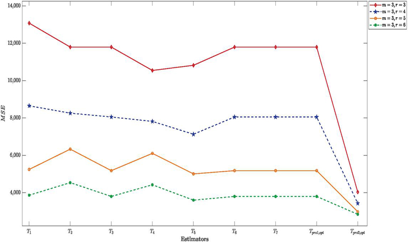
Figure 1 MSE of proposed and existing estimators for different values of $m$ and $r$ under empirical study.

5.2 Simulation Study

To analyze the performance of the proposed estimators under a more flexible environment, a simulation study has been conducted. An artificial population is generated using the following variable transformation. Similar transformations have been used by Bhushan et al., (2022). The transformations are given as follows:

$Y$	$=7.8+\sqrt{1-{\rho }^2}{Y}^{\ast }+\rho {\displaystyle \frac{S_Y}{S_X}}{X}^{\ast },$	(80)
$X$	$=7.2+X^{\ast }.$	(81)

Here, the variables $X^{\ast }$ and $Y^{\ast }$ are linearly independent and follow normal distributions with parameters $({\mu }_{X^{\ast }}=24,{\sigma }_{X^{\ast }}^2=37)$ and $({\mu }_{Y^{\ast }}=18,{\sigma }_{Y^{\ast }}^2=22)$, respectively.

The simulation study is performed for different values of the correlation coefficient $\rho =(0.4,0.5,0.7,0.8)$ with $10,000$ iterations. For each estimator, the MSE and PRE are computed to evaluate their performance.

The Percentage Relative Efficiency of an estimator $A$ with respect to estimator $B$ is defined as

$$PRE=\frac{MSE(B)}{MSE(A)}\times 100.$$

(82)

Here, $B$ represents the estimator $T_1$, while $A$ represents the estimators $T_1,T_2,T_3,T_4,T_5,T_6,T_7,T_{pro1,opt}$, and $T_{pro2,opt}$.

Table 2 MSE and PRE of the existing and proposed estimators for $\rho =0.8$ under simulation study

	m $=$ 3, r $=$ 3		m $=$ 3, r $=$ 4		m $=$ 3, r $=$ 5		m $=$ 3, r $=$ 6
Estimator	MSE	PRE	MSE	PRE	MSE	PRE	MSE	PRE
$T_1$ (Usual RSS)	89.3441	100	70.8380	100	63.8804	100	54.4197	100
$T_2$ (Muttlak and McDonald, (1992))	66.5486	134.2540	52.9277	133.8392	51.1348	124.9256	43.4527	125.2390
$T_3$ (Philip and Lam, (1997))	55.2797	161.6218	46.2386	153.2011	46.0097	138.8413	39.8008	136.7303
$T_4$ (Kadilar et al., (2009))	55.1479	162.0081	46.0948	153.6791	45.6477	139.9422	39.6910	137.1083
$T_5$ (Vishwakarma et al., (2017))	51.2205	174.4302	41.4400	170.9410	41.7385	153.0492	35.5892	152.9109
$T_6$ (Mehta et al., (2020))	55.2797	161.6218	46.2386	153.2011	46.0097	138.8413	39.8008	136.7303
$T_7$ (Khalid et al., (2024))	55.2797	161.6218	46.2386	153.2011	46.0097	138.8413	39.8008	136.7303
$T_{pro1,opt}$	55.2797	161.6218	46.2386	153.2011	46.0097	138.8413	39.8008	136.7303
$T_{pro2,opt}$	49.6095	180.0947	36.2619	195.3510	29.3704	217.4991	24.4384	222.6810

Figure 2 PRE of proposed and existing estimators for $\rho =0.8$ under simulation study for different values of $m$ and $r$

Table 3 MSE and PRE of the existing and proposed estimators for $\rho =0.7$ under simulation study

	m $=$ 3, r $=$ 3		m $=$ 3, r $=$ 4		m $=$ 3, r $=$ 5		m $=$ 3, r $=$ 6
Estimator	MSE	PRE	MSE	PRE	MSE	PRE	MSE	PRE
$T_1$ (Usual mean)	94.6245	100	75.5089	100	62.5240	100	53.2062	100
$T_2$ (Muttlak and McDonald, (1992))	80.6787	117.2857	64.3309	117.3757	53.1254	117.6914	45.1190	117.9242
$T_3$ (Philip and Lam, (1997))	67.2426	140.7212	56.3901	133.9046	48.0770	130.0496	41.6408	127.7742
$T_4$ (Kadilar et al., (2009))	66.6196	142.0370	55.7648	135.4061	47.6707	131.1582	41.3439	128.6918
$T_5$ (Vishwakarma et al., (2017))	63.7683	148.3881	51.8256	145.6981	43.1931	144.7545	36.8981	144.1975
$T_6$ (Mehta et al., (2020))	67.2426	140.7212	56.3901	133.9046	48.0770	130.0496	41.6408	127.7742
$T_7$ (Khalid et al.,(2024))	67.2426	140.7212	56.3901	133.9046	48.0770	130.0496	41.6408	127.7742
$T_{pro1,opt}$	67.2426	140.7212	56.3901	133.9046	48.0770	130.0496	41.6408	127.7742
$T_{pro2,opt}$	53.8578	175.6933	39.2805	192.2299	31.0183	201.5712	25.5727	208.0586

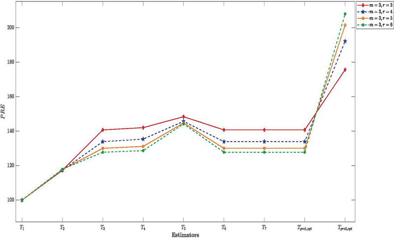
Figure 3 PRE of proposed and existing estimators for $\rho =0.7$ under simulation study for different values of $m$ and $r$

Table 4 MSE and PRE of the existing and proposed estimators for $\rho =0.5$ under simulation study

	m $=$ 3, r $=$ 3		m $=$ 3, r $=$ 4		m $=$ 3, r $=$ 5		m $=$ 3, r $=$ 6
Estimator	MSE	PRE	MSE	PRE	MSE	PRE	MSE	PRE
$T_1$ (Usual RSS)	101.2518	100	81.0265	100	67.1538	100	57.3233	100
$T_2$ (Muttlak and McDonald, (1992))	102.9256	98.3738	81.3525	99.5993	67.0076	100.2182	56.8822	100.7755
$T_3$ (Philip and Lam, (1997))	81.4335	124.3368	68.1680	118.8628	58.0229	115.7367	50.3180	113.9219
$T_4$ (Kadilar et al., (2009))	84.8590	119.3177	70.1981	115.4255	59.8195	112.2606	51.8752	110.5023
$T_5$ (Vishwakarma et al., (2017))	82.4069	122.8681	66.4900	121.8626	55.3405	121.3466	47.2942	121.2059
$T_6$ (Mehta et al., (2020))	81.4335	124.3368	68.1680	118.8628	58.0229	115.7367	50.3180	113.9219
$T_7$ (Khalid et al.,(2024))	81.4335	124.3368	68.1680	118.8628	58.0229	115.7367	50.3180	113.9219
$T_{pro1,opt}$	81.4335	124.3368	68.1680	118.8628	58.0229	115.7367	50.3180	113.9219
$T_{pro2,opt}$	64.3715	157.2928	46.3713	174.7341	36.3096	184.9476	29.7829	192.4703

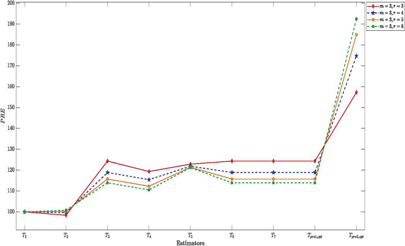
Figure 4 PRE of proposed and existing estimators for $\rho =0.5$ under simulation study for different values of $m$ and $r$.

Table 5 MSE and PRE of the existing and proposed estimators for $\rho =0.4$ under simulation study

	m $=$ 3, r $=$ 3		m $=$ 3, r $=$ 4		m $=$ 3, r $=$ 5		m $=$ 3, r $=$ 6
Estimator	MSE	PRE	MSE	PRE	MSE	PRE	MSE	PRE
$T_1$ (Usual mean)	103.0636	100	82.7107	100	68.6548	100	58.6429	100
$T_2$ (Muttlak and McDonald, (1992))	112.0692	91.9642	88.3273	93.6411	72.6570	94.4916	61.6551	95.1144
$T_3$ (Philip and Lam, (1997))	85.4026	120.6797	71.7155	115.3317	61.0000	112.5488	52.8971	110.8621
$T_4$ (Kadilar et al., (2009))	92.6269	111.2674	76.2349	108.4945	64.7902	105.9647	56.1568	104.4270
$T_5$ (Vishwakarma et al., (2017))	89.7932	114.7788	72.3225	114.3637	60.0786	114.2749	51.3559	114.1891
$T_6$ (Mehta et al., (2020))	85.4026	120.6797	71.7155	115.3317	61.0000	112.5488	52.8971	110.8621
$T_7$ (Khalid et al.,(2024))	85.4026	120.6797	71.7155	115.3317	61.0000	112.5488	52.8971	110.8621
$T_{pro1,opt}$	85.4026	120.6797	71.7155	115.3317	61.0000	112.5488	52.8971	110.8621
$T_{pro2,opt}$	69.4723	148.3520	49.8040	166.0725	39.0837	175.6608	31.9675	183.4450

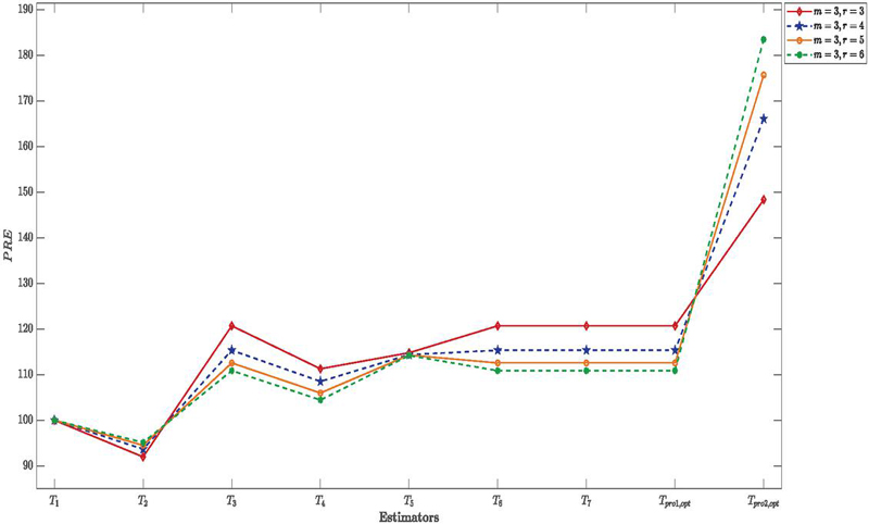
Figure 5 PRE of proposed and existing estimators for $\rho =0.4$ under simulation study for different values of $m$ and $r$.

6 Results & Discussion

The major findings of the study can be summarized as follows:

1. In the Table 1, under the empirical study, the suggested estimator ($T_{pro1}$) achieves an MSE of $11793.2170$ ($(m=3,r=3)$), which is precisely the same as that of the regression estimator ($T_7$). This shows that, given the examined circumstances, the estimate $T_{pro1}$ is theoretically as efficient as the current regression estimator. However, of all the conventional estimators taken into consideration in this study, the second suggested estimator $T_{pro2}$ produces a far lower MSE of $4031.5790$, making it the most effective estimator. Other parameter combinations $(m=3,r=4,5,6)$ show similar performance patterns. The stability of these results across various simulation settings is further confirmed by the results presented in Tables 2 to 5.

2. Tables 2 to 5 also show that the MSE of the suggested estimators steadily decreases as we move horizontally across the tables (i.e., with an increasing sample size). The PRE exhibits a growing trend in line with this. This tendency suggests that as sample sizes increase, the suggested estimators become more effective. The reader can consult Figures (2–-5), which show the behavior of the estimators for various values of the correlation coefficient $\rho$=$(0.8,0.7,0.5,$ and $0.4)$, to better see these tendencies.

3. Simulation results shown in Tables 2 to 5 suggest that the effectiveness of the suggested estimators increases with an increase in the correlation coefficient. In particular, the MSE values of the suggested estimators significantly reduce when the correlation between the study variable and the auxiliary variable rises from $\rho =0.4$ to $\rho =0.8$, but their PRE values rise proportionally. This finding implies that the suggested estimators improve the overall efficiency of estimation within the RSS framework, especially when the auxiliary variable has a strong correlation with the study variable.

4. Khalid et al. (2024) employed convex combination of ratio and exponential ratio estimator whereas our proposed second estimator ($T_{pro2,opt}$) employs linear combination which involves ratio-cum-product, regression type and exponential ratio and product estimators. Incorporation of regression form of estimator and exponential ratio-cum-product type estimator suggest that it will perform better than Khalid et al. (2024) which involve less efficient estimators Ratio and exponential ratio estimators. Hence, the fact that our proposed estimator involves more efficient estimators than those incorporated by Khalid et al. (2024) supports its better performance that we have already shown through empirical and simulation studies.

7 Conclusion

In order to create effective estimators for the finite population mean, we conducted a thorough theoretical and numerical examination within the framework of Ranked Set Sampling (RSS). Building a mathematical functional form that may generate an estimator with a significantly lower mean squared error (MSE) than the current estimators is a difficult challenge, according to a thorough analysis of the literature. The varied nature of populations and the disparate correlations between the research variable and the auxiliary data are the primary causes of this challenge. Thus, the creation of novel estimators that can attain higher efficiency in various sampling scenarios continues to be a crucial field of study.

Inspired by this goal, this study offered two novel estimators. Through a thorough simulation analysis and comparison with a number of conventional estimators found in the literature, their theoretical characteristics were investigated and their performance assessed. Overall, it is evident from both theoretical derivations and simulation experiments that the estimator $T_{pro2}$ consistently outperforms all of the conventional estimators taken into consideration in this study, but the estimator $T_{pro1}$ performs similarly to some of the current estimators. Therefore, when auxiliary data is provided, the suggested estimator $T_{pro2}$ can be suggested as a more effective substitute for estimating the finite population mean under Ranked Set Sampling. This research could be expanded to include more auxiliary variables and alternative sample strategies.

Conflict of Interest

The authors declare no competing interests.

Declaration of Competing Financial Interest

The authors declare that they have no known competing financial interests or personal relationships that could have appeared to influence the work reported in this paper.

Funding

The authors declare that no funds or other grants were received for the preparation of this manuscript.

Ethical Statement

There are no human/animal subjects in this article therefore an ethics statement is not applicable because this study is applied on already published data.

Data Availability Statement

All data applied is included in the manuscript.

Author Contribution Statement

All authors listed have contributed significantly to write this article.

References

Audu et al., (2025) Audu, A., Aphane, M., Ishaq, O. O., and Singh, R. V. K. (2025). New estimators of population variance based on logarithmic transformation in the presence of random non-response and measurement errors under successive sampling. Afrika Matematika, 36(2):104.

Bhushan and Kumar, (2022) Bhushan, S. and Kumar, A. (2022). Novel log type class of estimators under ranked set sampling. Sankhya B, 84(1):421–447.

Bhushan et al., (2022) Bhushan, S., Kumar, A., and Lone, S. A. (2022). On some novel classes of estimators using ranked set sampling. Alexandria Engineering Journal, 61(7):5465–5474.

Bhushan et al., (2023) Bhushan, S., Kumar, A., Zaman, T., and Al Mutairi, A. (2023). Efficient difference and ratio-type imputation methods under ranked set sampling. Axioms, 12(6):558.

Cochran, (1940) Cochran, W. G. (1940). The estimation of the yields of cereal experiments by sampling for the ratio of grain to total produce. The journal of agricultural science, 30(2):262–275.

Dell and Clutter, (1972) Dell, T. and Clutter, J. (1972). Ranked set sampling theory with order statistics background. Biometrics, pages 545–555.

Djebar et al., (2026) Djebar, A., Alghamdi, A. S., Mustafa, M. S., and Ahmad, S. (2026). Computation of population variance estimation in simple random sampling structures by developing generalized estimator. Mathematics, 14(2):375.

Halls and Dell, (1966) Halls, L. K. and Dell, T. R. (1966). Trial of ranked-set sampling for forage yields. Forest Science, 12(1):22–26.

Jafari Jozani and Johnson, (2011) Jafari Jozani, M. and Johnson, B. C. (2011). Design based estimation for ranked set sampling in finite populations. Environmental and Ecological Statistics, 18(4):663–685.

Kadilar et al., (2009) Kadilar, C., Unyazici, Y., and Cingi, H. (2009). Ratio estimator for the population mean using ranked set sampling. Statistical Papers, 50(2): 301–309.

Khalid et al., (2024) Khalid, E. G. et al. (2024). Generalized exponential ratio type estimator for the finite population mean under ranked set sampling. Pakistan Journal of Statistics and Operation Research, pages 409–417.

Khalid et al., (2022) Khalid, R., Koçyiğit, E. G., and Ünal, C. (2022). New exponential ratio estimator in ranked set sampling. Pakistan Journal of Statistics and operation research, pages 403–409.

Kumari et al., (2024) Kumari, A., Singh, R., and Smarandache, F. (2024). New modification of ranked set sampling for estimating population mean: neutrosophic median ranked set sampling with an application to demographic data. International Journal of Computational Intelligence Systems, 17(1):210.

Kumari et al., (2025) Kumari, M., Sharma, P., Singh, P., and Ozel, G. (2025). Enhanced mean estimation using memory type estimators with dual auxiliary variables: Accepted-january 2025. REVSTAT-Statistical Journal.

Lynne Stokes, (1977) Lynne Stokes, S. (1977). Ranked set sampling with concomitant variables. Communications in Statistics-Theory and Methods, 6(12):1207–1211.

McIntyre, (1952) McIntyre, G. (1952). A method for unbiased selective sampling, using ranked sets. Australian journal of agricultural research, 3(4):385–390.

Mehta et al., (2020) Mehta, V., Singh, H. P., and Pal, S. K. (2020). A general procedure for estimating finite population mean using ranked set sampling. Rev. Invest. Oper, 41(1):80–92.

Muttlak and McDonald, (1992) Muttlak, H. and McDonald, L. (1992). Ranked set sampling and the line intercept method: A more efficient procedure. Biometrical Journal, 34(3):329–346.

Philip and Lam, (1997) Philip, L. and Lam, K. (1997). Regression estimator in ranked set sampling. Biometrics, pages 1070–1080.

Samawi and Muttlak, (1996) Samawi, H. M. and Muttlak, H. A. (1996). Estimation of ratio using rank set sampling. Biometrical Journal, 38(6):753–764.

Sharma et al., (2025) Sharma, P., Singh, P., Kumari, M., and Singh, R. (2025). Estimation procedures for population mean using ewma for time scaled survey. Sankhya B, 87(1):103–128.

Shukla et al., (2026) Shukla, D., Gupta, V. K., and Jain, A. (2026). A class of logarithmic exponential estimators for estimating average degree of a network using triangular graph sampling. Communications in Statistics-Theory and Methods, 55(9):2777–2802.

Singh et al., (2024) Singh, P., Sharma, P., and Maurya, P. (2024). Enhancing accuracy in population mean estimation with advanced memory type exponential estimators. Journal of Reliability and Statistical Studies, pages 417–434.

Singh et al., (2025) Singh, P., Sharma, P., Singh, A., Zaman, T., and Emam, W. (2025). Log-transformed approaches to variance estimation using auxiliary data. Journal of Radiation Research and Applied Sciences, 18(4):101913.

Singh and Singh, (2026) Singh, P. and Singh, A. (2026). Simulation and real-world applications of exponential–log estimators under neutrosophic ranked set sampling. Statistics, pages 1–20.

Singh, (2003) Singh, S. (2003). Simple random sampling. In Advanced Sampling Theory with Applications: How Michael ‘selected’Amy Volume I, pages 71–136. Springer.

Takahasi and Wakimoto, (1968) Takahasi, K. and Wakimoto, K. (1968). On unbiased estimates of the population mean based on the sample stratified by means of ordering. Annals of the institute of statistical mathematics, 20(1):1–31.

Vishwakarma and Singh, (2022) Vishwakarma, G. K. and Singh, A. (2022). Generalized estimator for computation of population mean under neutrosophic ranked set technique: An application to solar energy data. Computational and applied mathematics, 41(4):144.

Vishwakarma et al., (2017) Vishwakarma, G. K., Zeeshan, S. M., and Bouza, C. N. (2017). Ratio and product type exponential estimators for population mean using ranked set sampling. Investigacion Operacional, 38(3):266 – 271. Cited by: 12.

Wolfe, (2012) Wolfe, D. A. (2012). Ranked set sampling: its relevance and impact on statistical inference. International scholarly research notices, 2012(1):568385.

Woodall et al., (2024) Woodall, W. H., Haq, A., Mahmoud, M. A., and Saleh, N. A. (2024). Reevaluating the performance of control charts based on ranked-set sampling. Quality Engineering, 36(2):365–370.

Zaman and Iftikhar, (2023) Zaman, T. and Iftikhar, S. (2023). A new logarithmic ratio type estimator of population mean for simple random sampling: a simulation study. Journal of Science and Arts, 23(4):839–848.

Zaman et al., (2024) Zaman, T., Itikhar, S., Sozen, C., and Sharma, P. (2024). A new logarithmic type estimators for analysis of number of aftershocks using poisson distribution. Journal of Science and Arts, 24(4):833–842.

Zarinkolah et al., (2024) Zarinkolah, M. H., Jabbari, H., and Saber, M. M. (2024). Optimal estimators of the population mean of a skewed distribution using auxiliary variables in median ranked-set sampling. Mathematical Population Studies, 31(1):62–85.

Zubair et al., (2024) Zubair, M., Yasin, S., Al-Bossly, A., Ali, A., Al Samman, F. M., A. Almazah, M. M., and Iqbal, K. (2024). Double extreme-cum-median ranked set sampling. PloS one, 19(12):e0312140.

Biographies

Poonam Singh is an Assistant Professor in the Department of Statistics, Institute of Science, at Banaras Hindu University. She obtained her B.Sc. (Hons.), M.Sc., and Ph.D. in Statistics from Banaras Hindu University and served as a Visiting Fellow at University of Technology Sydney in 2025. Her research interests include sampling theory, applied statistics, neutrosophic theory, and machine learning. Dr. Singh has published numerous research articles in reputed international journals indexed in SCIE, ESCI, and Scopus, and has authored a scholarly book on survey sampling. She has successfully supervised postgraduate research and is currently guiding doctoral scholars. She is a recipient of the Global Experience Faculty Program Fellowship and the Institute of Eminence (IoE) Research Grant from BHU. Dr. Singh actively serves as a reviewer for several international journals and is a member of professional organizations including the Indian Society of Probability and Statistics, the Epidemiology Foundation of India, and the Indian Bayesian Society.

Sooraj Gupta is a Research Scholar in the Department of Statistics at Banaras Hindu University. He completed his Bachelor’s and Master’s degrees in Statistics from the same institution with distinction. His doctoral research focuses on the development of efficient estimators for finite population parameters using auxiliary information in survey sampling. His research interests include survey sampling, ranked set sampling, estimation theory, and statistical applications in agriculture and socio-economic studies. He has published research in internationally indexed journals, including Neutrosophic Sets and Systems and REVSTAT–Statistical Journal. He is proficient in R, Python, SPSS, and statistical computing tools, and has qualified national-level examinations such as JAM and GATE in Statistics.

Pooja Maurya is a Research Scholar in the Department of Statistics at Banaras Hindu University, where she is pursuing her Ph.D. under the supervision of Dr. Poonam Singh. She obtained her M.Sc. in Statistics from Banaras Hindu University with a CGPA of 9.11 and her B.Sc. in Mathematics, Statistics, and Computer Science from Deen Dayal Upadhyaya Gorakhpur University. Her research interests lie in sampling theory, particularly in developing efficient estimators for population parameters using auxiliary information in time-scaled surveys. She has authored several publications in internationally indexed journals and has served as a reviewer for leading statistical journals. Her expertise includes statistical computing and data analysis using R, Python, MATLAB, Stata, and LaTeX.

Prayas Sharma is an Assistant Professor in the Department of Statistics, School of Physical and Decision Science, at Babasaheb Bhimrao Ambedkar University. He earned his Ph.D. in Statistics from Banaras Hindu University and has over 12 years of teaching and 13 years of research experience. His research interests include sampling theory, predictive modeling, business analytics, artificial intelligence and machine learning, applied statistics, and energy sustainability. Dr. Sharma has authored more than 50 research papers in reputed international journals indexed in SCIE, ESCI, Scopus, and ABDC databases, along with a book and several book chapters. He serves on the editorial boards of several international journals and actively reviews manuscripts for leading statistical and interdisciplinary journals. He is a member of professional bodies including the International Indian Statistical Association (IISA) and the Indian Society for Probability and Statistics (ISPS).

Journal of Reliability and Statistical Studies, Vol. 19, Issue 2 (2026), 311–346.
doi: 10.13052/jrss0974-8024.1924
© 2026 River Publishers