Comparing Classical and Sequential Parameter Estimation in Power Rayleigh Distribution

Prem Lata Gautam

Amity School of Applied Sciences, Amity University, Lucknow, Uttar Pradesh-226028, India
E-mail: plgautam@lko.amity.edu

Received 30 January 2026; Accepted 09 June 2026

Abstract

This study explores the novel application of the performance characteristics of sequential probability ratio test (SPRT) for estimation the scale parameter ($\theta$) of the power Rayleigh distribution, focusing on its scale parameters ($\theta$) that are the fundamental to defining its properties and shaping the statistical characteristics. For testing the null hypothesis $H_0:\theta ={\theta }_0$ versus $H_1:\theta ={\theta }_1$, a stop rule method is utilized to optimize the sample size. Through this approach, we derive approximations for key performances metrics, including the operating characteristic (OC) function and the average sample number (ASN). The study also confirms the existence of the function $L(\theta )$, necessary to meet the ASN requirements in sequential testing. The new method is comprised of the efficiency of the SPRT compared to the classical Neyman-Pearson (N-P) technique. A comprehensive simulation study shows that the proposed method of SPRT significantly reduces the sample size required for the hypothesis testing by 65.99% to 77.49% compared to the Neyman-Pearson (N-P) test without compromising accuracy.

Keywords: Sequential probability ratio test, operating characteristics, average sample number, acceptance and rejection regions, power Rayleigh distribution, Neyman-Pearson procedure, Type I error and Type II error.

1 Introduction

The original purpose of sequential analysis, firstly developed by Wald (1947), was to improve quality control during World War II. This goal was accomplished to such an extent that it was instantly classified. Sequential analysis tries to minimize the sample size while maintaining decision-making ability by treating it as a random variable for that specific method. This is achieved by stopping data collecting after one more observation has been made in order to determine whether a choice can be made. There are several uses for the potential to lower the sample size needed to decide on an experiment because this methodology conserves resources and makes financing more easily obtained.

Since, Wald (1947), numerous sequential tests have been suggested to evaluate various hypotheses. For instance, in the books Whitehead and Jones (1983) and Jennison and Turnbull (2000) offered various applications of sequential and group sequential method-based methodologies to the design and implementation of clinical trials. For further information, readers can referred to their books.

Darkhovsky (2011) proposed a sequential approach that minimizes the Bayesian risk maximum over a variety of prior parameter distributions in order to study the problem of sequential testing for two composite hypotheses. Tartakovsky et al. (2015) went into great detail about current advancements by developing the systematic hypothesis testing and change point detection in the theory of sequential analysis in their book . Kharin (2016) looked on the reliability and efficiency of sequential testing. Nakamura et al. (2016) suggested a sequential test that find the lowest dose that has a threshold effect.

A universal sequential test was developed by Li et al. (2017) to identify outliers in all of the gathered observation sequences. An ideal truncated group sequential test for binomial proportions was proposed by Hu and Wang (2018). The study of Dyrssen and Ekstrom (2018) examined the sequential testing of two simple hypothesis for the shift of a Brownian motion with expensive observations. Zou et al. (2019) presented a nonparametric sequential test based on empirical likelihood to assess for treatment effects.

Likelihood ratio test method is widely applicable method for the two simple/composite hypothesis with a fixed sample size. For example, Self and Liang (1987) obtained the asymptotic distribution of maximum likelihood ratio statistics under nonstandard conditions. Fan and Zhang (2004) gave the empirical likelihood ratio test for non-parametric functions. Ferrari and Cysneiros (2008) applied the modified likelihood ratio method to study the exponential family nonlinear model and get the modified likelihood ratio statistics. Giampaoli and Singer (2009) used likelihood ratio method to estimated the variance parameter of the linear mixed model. Huang et al. (2013) used the Lq-likelihood ratio method for the testing of shape parameter of the generalized extremum distribution. Similar method is propsed by Qin and Priebe (2017) for the general pollution distribution also obtained the asymptotic distribution of Lq-likelihood ratio test statistics.

The presented work shows the importance of the sequential testing procedure compared with the classical fixed-sample methods, as SPRT offers a more flexible approach. In this case, the power Rayleigh distribution which is applied in survival studies, reliability analysis, and communication systems, SPRT has shown better performance than classical procedures due to its faster convergence and lower average sample size. Therefore, the comparison between SPRT and classical methods under the power Rayleigh distribution is of considerable practical and theoretical importance in statistical analysis and real-time applications.

2 SPRT Procedure

Wald (1947) introduced a extension of the sequential estimation by introducing the sequential probability ratio test (SPRT). Consider a sequence of i.i.d random variable $X_1,X_2,\mathrm{\dots }$ having the common probability density function (p.d.f) $f(x|\theta )$, $\theta \in \mathrm{\Theta }$. To testing the one simple null hypothesis $H_0:\theta ={\theta }_0$ against the alternative $H_1:\theta ={\theta }_1$, where ${\theta }_0\ne {\theta }_1$ are two specified numbers in the parameter space $\mathrm{\Theta }$. We also have two preassigned numbers $0<\alpha ,\beta <1$, and corresponding to type I and type II error probabilities.

Let $X_n=(X_1,X_2,\mathrm{\dots }{X}_n)$, when $\theta$ is true parameter value, the likelihood function of $X_n$ is

$$L(X_n,\theta )={\mathrm{\Pi }}_{i=1}^{n}f(X_i,\theta )$$

We denote $L_0(i)={\mathrm{\Pi }}_{i=1}^{n}f(X_i,{\theta }_0)$ and $L_1(i)={\mathrm{\Pi }}_{i=1}^{n}f(X_i,{\theta }_1)$, respectively under $H_0$ and $H_1$. The most powerful (MP) level $\alpha$ test has the form

$$\text{Reject}{H}_0\text{if and only if}\frac{L_1(i)}{L_0(i)}\ge k$$

(1)

where $k>0$ is to be determined appropriately.

The test (1) is the best among all fixed sample size ($=$i) tests at level $\alpha$. But its type II error probability can be quite bit larger than $\beta$. In order to meet both $(\alpha ,\beta )$ requirements. Abraham Wald (1940) looked at this problem from a different angle. Having observed $X_n$ let us consider the sequence of successive likelihood ratios is defined as:

$${\mathrm{\Lambda }}_i=\frac{L_1(i)}{L_0(i)}i=1,2,3\mathrm{\dots }$$

In other words, we observe $X_1,X_2,X_3,\mathrm{\dots }$ one by one and accordingly obtain ${\mathrm{\Lambda }}_1,{\mathrm{\Lambda }}_2,{\mathrm{\Lambda }}_3,\mathrm{\dots }$ in a sequential manner. As soon as we find one ${\mathrm{\Lambda }}_j$ in the sequence that appears too small or too large we quit sampling, and we decide in favor of $H_0(or{H}_1)$ whenever ${\mathrm{\Lambda }}_i$ is too small (or too large), $\mathrm{i}=1,2,\mathrm{\dots }.$

By choosing two constants A and B such that $0<B<A<\mathrm{\infty }$, sequential probability ratio test (SPRT) is then implemented as –

We continue observing $X_1,X_2,\mathrm{\dots }$ one by one in a sequence until the likelihood ratio ${\mathrm{\Lambda }}_i$ goes out of the interval (B, A) for the first time then accept $H_0$ if ${\mathrm{\Lambda }}_i\le B$, reject $H_0$ if ${\mathrm{\Lambda }}_i\ge A$ and continue sampling if $B<{\mathrm{\Lambda }}_i<A$ for $i=1,2,\mathrm{\dots }n$ number of experiments. The constants A and B are computed using the values of Type I and Type II error probabilities $\alpha$ and $\beta$. The mathematical formula of A and B is defined as $A=(1-\beta )/\alpha$ and $B=\beta /(1-\alpha )$. The performance of SPRT can be measured by the two criteria one is Operating Characteristic (OC) fuction and another is Average sample number (ASN).

Operating Characteristic (OC) fuction denotes the probability that the sequential test will lead to the acceptance of the hypothesis $H_0:\theta ={\theta }_0$ when $\theta$ is the true value. It is denoted as $L(\theta )$ and relates how well the test procedures achieves its objective of making correct decisions. The number of observation N required by a sequential procedure to reach a decision is not predetermined but a random variable. If we repeat the same sequential then we shall get different values N. Small value of N on an average is preferable. This average value of N is called the Average Sample Number (ASN). Wald (1947) suggested the mathematical formula for the OC and ASN as –

$$L(\theta )=\frac{A^h-1}{A^h-B^h}$$

(2)

where A and B are constants, depends on the Type I and Type II error of probabilities both, and ‘$h$’ is the solution of non-zero equation and is given as

$$E{[e^{Z_i}]}^h=1$$

(3)

the ASN function under $H_0$ and $H_1$ is given by

$E_0(N)=$	${\displaystyle \frac{(1-\alpha )\ln B+\alpha \ln A}{E(Z_i)}}$	(4)
$E_1(N)=$	${\displaystyle \frac{\beta \ln B+(1-\beta )\ln A}{E(Z_i)}}$

where, $Z_i=log(f(X_n,{\theta }_1)/f(X_i,{\theta }_0))$ provided $E(Z_i)\ne 0$.

SPRT is applied by various author, one may referred to Chaturvedi et al.(2000), Sevil and Demirhan (2008), Pandit and Gudaganavar (2010), Kharin (2016), Ning and Opperman (2019) and Surinder.K et al. (2022).

The acceptance and rejection regions are crucial when statistical decision under SPRT are depends on the data. Similar to classical theory, rejection region indicate strong evidence against the null hypothesis and acceptance region signifies the values for which the null hypothesis can not be rejected.

Rayleigh (1880) introduced a distribution, named Rayleigh distribution with many applications in the field of engineering and medical disciplines for data modeling. It is often applied in hydrology to model phenomena that involves the magnitude of extreme or varying value, such as wave heights, riven flow velocity and wind speeds over water bodies. To enhance the flexibility of Rayleigh model Power transformation $x=y^{\frac{1}{\nu }}$ is used. The cumulative distribution function (CDF) of the X is presented by

$$F(x)=P(X\le x)=P(Y\le x^{\nu })=F_y(x^{\nu })$$

Thus, the probability density function (PDF) and cumulative density function (CDF) of power Rayleigh (PR) distribution is given by –

$f(x)$

$={\displaystyle \frac{\nu }{{\theta }^2}}{x}^{2\nu -1}{e}^{\frac{-x^{2\nu }}{2{\theta }^2}}x>0,\theta ,\nu >0,F(x)=1-e^{\frac{-x^{2\nu }}{2{\theta }^2}}$

(5)

where, $\theta$ is scale parameter and $\nu$ is shape parameter. The presented study deal with the estimation of scale parameter of the power Rayleigh distribution.

3 Sequential Probability Ratio Test (SPRT) for Power Rayleigh Distribution

Suppose that $X_1,X_2,X_3,\mathrm{\dots }$ be an independent and identically distributed random sample from the pdf (5). Here, testing the null hypothesis $H_0:\theta ={\theta }_0$ $vs.$ an alternative $H_1:\theta ={\theta }_1$.The test statistic for the test SPRT is defined as –

${\mathrm{\Lambda }}_n$	$={\left({\displaystyle \frac{{\theta }_0}{{\theta }_1}}\right)}^{2}exp\left[-{\displaystyle \frac{x^{2\nu }}{2}}\left({\displaystyle \frac{1}{{\theta }_0^2}}-{\displaystyle \frac{1}{{\theta }_1^2}}\right)\right]$
$\ln {\mathrm{\Lambda }}_n$	$=2\text{ln}\left({\displaystyle \frac{{\theta }_0}{{\theta }_1}}\right)+{\displaystyle \frac{x^{2\nu }}{2}}\left({\displaystyle \frac{1}{{\theta }_1^2}}-{\displaystyle \frac{1}{{\theta }_0^2}}\right)$	(6)

The decision rule is defined as –

1. Accept $H_0$ if ${\mathrm{\Lambda }}_n={\left(\frac{{\theta }_0}{{\theta }_1}\right)}^{2}exp\left[-\frac{x^{2\nu }}{2}\left(\frac{1}{{\theta }_0^2}-\frac{1}{{\theta }_1^2}\right)\right]\le B$

2. Reject $H_0$ if ${\mathrm{\Lambda }}_n={\left(\frac{{\theta }_0}{{\theta }_1}\right)}^{2}exp\left[-\frac{x^{2\nu }}{2}\left(\frac{1}{{\theta }_0^2}-\frac{1}{{\theta }_1^2}\right)\right]\ge A$

3. Continue taking sampling if $B<{\left(\frac{{\theta }_0}{{\theta }_1}\right)}^{2}exp\left[-\frac{x^{2\nu }}{2}\left(\frac{1}{{\theta }_0^2}-\frac{1}{{\theta }_1^2}\right)\right]<A$

4 Operating Characteristic (OC) for SPRT

As, from the decision rule, SPRT method depends on the pre-defined constants $A$ and $B$. So, by selecting $A$ and $B$, we are studying the properties of SPRT that can be turned into the study of random walks. In this Section, some characteristic of SPRT are derived for the pdf of (5).

Let to test $H_0:\theta ={\theta }_0$ against the hypothesis $H_1:\theta ={\theta }_1$, with the given constants $\alpha$ and $\beta$, suppose $\nu$ is known. To find the OC function we obtained the value of $Z_i$ as

$Z_i$	$=\ln \left({\displaystyle \frac{f(X_i,{\theta }_1)}{f(X_i,{\theta }_0)}}\right)$
	$=\ln {\left({\displaystyle \frac{{\theta }_0}{{\theta }_1}}\right)}^2\exp [-{\displaystyle \frac{x^{2\nu }}{2}}({\displaystyle \frac{1}{{\theta }_1^2}}-{\displaystyle \frac{1}{{\theta }_0^2}})]$
	$=2\ln {\displaystyle \frac{{\theta }_0}{{\theta }_1}}-{\displaystyle \frac{x^{2\nu }}{2}}\left({\displaystyle \frac{1}{{\theta }_1^2}}-{\displaystyle \frac{1}{{\theta }_0^2}}\right)$	(7)

From the equations, (3) and (4), we have

$$E{\left[e^{Z_i}\right]}^h=\frac{{\left(\frac{{\theta }_0}{{\theta }_1}\right)}^{2h}}{\left[h{\theta }^2\left(\frac{1}{{\theta }_1^2}-\frac{1}{{\theta }_0^2}\right)+1\right]}$$

(8)

To solve this equation, taking logarithm and using the expression $\ln (1+x);-1<x<1$ in (3.4). Expanding the terms up to third degree we got the quadratic equation in ‘h’ –

	${\displaystyle \frac{h^2}{3}}{\left[{\theta }^2\left({\displaystyle \frac{1}{{\theta }_1^2}}-{\displaystyle \frac{1}{{\theta }_0^2}}\right)\right]}^3-{\displaystyle \frac{h}{2}}{\left[{\theta }^2\left({\displaystyle \frac{1}{{\theta }_1^2}}-{\displaystyle \frac{1}{{\theta }_0^2}}\right)\right]}^2$
	$+{\theta }^2\left({\displaystyle \frac{1}{{\theta }_1^2}}-{\displaystyle \frac{1}{{\theta }_0^2}}\right)-2\ln \left({\displaystyle \frac{{\theta }_0}{{\theta }_1}}\right)=0$	(9)

After solving the (4), numerical values of OC function under the scale parameter of power Rayleigh distribution is obtained. For testing $H_0:\theta =12$ vs $H_1:\theta =14$ with $\alpha =\beta =0.05$.The numerical values of OC functions are represented in Table 1 and curve are plotted in Figure 1. The resulted numerical values at $\theta =12$ and $\theta =14$ are near to and 0.95 and 0.05 are satisfactory.

Table 1 Numerical value for OC function under $H_0:\theta =12$ vs $H_1:\theta =14$ with $\alpha =\beta =0.05$

$\theta$	$L(\theta )$	$\theta$	$L(\theta )$
11.0	0.999	12.7	0.67
11.1	0.999	12.8	0.6
11.2	0.998	12.9	0.527
11.3	0.997	13.0	0.453
11.4	0.996	13.1	0.382
11.5	0.993	13.2	0.317
11.6	0.99	13.3	0.258
11.7	0.985	13.4	0.206
11.8	0.978	13.5	0.163
11.9	0.968	13.6	0.126
12.0	0.954	13.7	0.096
12.1	0.936	13.8	0.082
12.2	0.911	13.9	0.063
12.3	0.88	14.0	0.057
12.4	0.84	14.1	0.025
12.5	0.792	14.2	0.016
12.6	0.735	14.3	0.008

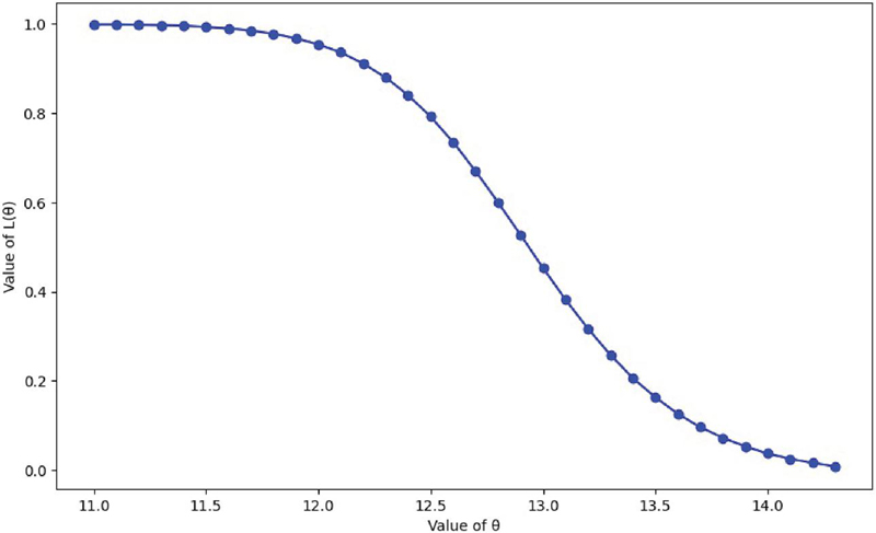
Figure 1 OC function curve for Power Rayleigh distribution.

5 Average Sample Number (ASN) for the SPRT

In a sequential estimation procedure, the sample size required to make a decision is denoted by $N$. The true distribution of the observations made throughout the sampling procedure determines how this random variable will be distributed. The function of ASN, approximately represented as

$$E(N|\theta )=\frac{L(\theta )\ln B+[1-L(\theta )]\ln A}{E(Z)}$$

(10)

also given that $E(Z)\ne 0$, where

$$E(Z)=2\ln \left(\frac{{\theta }_0}{{\theta }_1}\right)-{\theta }^2\left(\frac{1}{{\theta }_1^2}-\frac{1}{{\theta }_0^2}\right)$$

(11)

where, $E[x^{2\nu }]=2{\theta }^2$ (Mahmoud, et al., 2020).

From Equation (4), the function of ASN under $H_0$ and $H_1$ is represented as

$$E_0(N)=\frac{(1-\alpha )\ln B+\alpha \ln A}{2\ln \left(\frac{{\theta }_0}{{\theta }_1}\right)-{\theta }_0^2\left(\frac{1}{{\theta }_1^2}-\frac{1}{{\theta }_0^2}\right)}$$

(12)

and

$$E_1(N)=\frac{\beta \ln B+(1-\beta )\ln A}{2\ln \left(\frac{{\theta }_0}{{\theta }_1}\right)-{\theta }_1^2\left(\frac{1}{{\theta }_1^2}-\frac{1}{{\theta }_0^2}\right)}$$

(13)

After solving the (13), numerical values of ASN function under the scale parameter of power Rayleigh distribution is obtained. For testing $H_0:\theta =12$ vs $H_1:\theta =14$ with $\alpha =\beta =0.05$, the numerical values of ASN functions (10) are represented in Table 2 and curve are plotted in Figure 2. The ASN curve is a plotted against the values of $\theta$. The Table and Curve gives satisfactorily results.

Table 2 Numerical value for ASN function under $H_0:\theta =12$ vs $H_1:\theta =14$ with $\alpha =\beta =0.05$

$\theta$	E(N)	$\theta$	E(N)
11.0	34.446	12.7	89.970
11.1	36.142	12.8	91.337
11.2	38.016	12.9	91.470
11.3	40.092	13.0	90.363
11.4	42.395	13.1	88.126
11.5	44.951	13.2	84.958
11.6	47.787	13.3	81.106
11.7	50.924	13.4	76.819
11.8	54.380	13.5	72.326
11.9	58.156	13.6	67.808
12.0	62.239	13.7	63.401
12.1	66.581	13.8	59.195
12.2	71.097	13.9	55.246
12.3	75.656	14.0	51.580
12.4	80.068	14.1	48.205
12.5	84.100	14.2	45.120
12.6	87.487	14.3	42.332

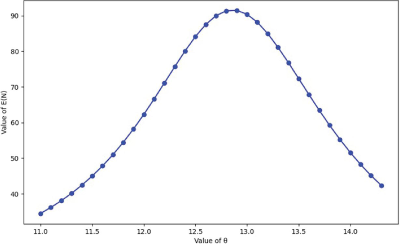
Figure 2 ASN function curve for Power Rayleigh distribution.

The ASN is maximized for intermediate values of $\theta$ because in the midrange, the observations would support neither hypothesis with strong confidence, which would increase the number of observations needed to make a decision to accept or reject the hypothesis. If $\theta$ is near ${\theta }_0$ and near ${\theta }_1$, on the other hand, the generated data bolster one alternative hypothesis, causing the test statistic to cross the respective boundaries earlier than it would if $\theta$ were different, and there will be fewer average sample sizes. Therefore, the greater the difficulty in distinguishing between the hypotheses, the larger the ASN, and the closer it comes to the parameter values that correspond to making better decisions, the smaller it becomes.

6 Acceptance and Rejection region

Here, we define, $Y(n)={\sum }_{i=1}^n{X}_i^{2\nu }$ and N=first integer $n(\ge 1)$, for which the inequality $Y(n)\le c_1+dn$ or $Y(n)\ge c_2+dn$ holds with the constants

$c_1={\displaystyle \frac{\ln B}{\frac{1}{2}\left(\frac{1}{{\theta }_1^2}-\frac{1}{{\theta }_0^2}\right)}},c_2={\displaystyle \frac{\ln A}{\frac{1}{2}\left(\frac{1}{{\theta }_1^2}-\frac{1}{{\theta }_0^2}\right)}}\text{and}d={\displaystyle \frac{2\ln \frac{{\theta }_0}{{\theta }_1}}{\frac{1}{2}\left(\frac{1}{{\theta }_1^2}-\frac{1}{{\theta }_0^2}\right)}}$

The decision rule for the SPRT is

1. when $Y_n\ge c_1+\text{dn}$, we have to stop the experiment and accept $H_0$

2. when $Y_n\le c_1+\text{dn}$, we have to stop the experiment and reject $H_0$

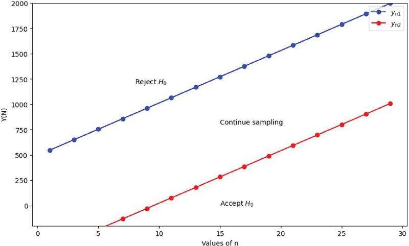
Figure 3 Acceptance and Rejection region.

Remarks: The Figure 3, shows the acceptance and rejection regions for $H_0$ under the case when $H_0:{\theta }_0=12$ vs $H_1:{\theta }_1=14$ for $\alpha =\beta =0.05$. The values of constants $c_1=494.6657$, $c_2=-494.6657$ and $d=51.79463$, respectively. Thus, if $Y(N)\le 494.6657N+51.79463$, we accept $H_0$ and if $Y(N)\ge -494.6657N+51.79463$, we accept $H_1$. At the intermediate stages, we continue sampling.

7 Fixed-Sample Size Procedure

Let $\{X_i\}$ be i.i.d. having the pdf (5). We are interested to $H_0:\theta ={\theta }_0$ against the alternative $H_1:\theta ={\theta }_1$. For the estimation of fixed-sample size we are using Neyman-Pearson test method. As per N-P method, the optimal fixed quantity is defined as where, $n$ and $K$ satisfy

$P_{{\theta }_0}(\overline{X}\ge K)$	$=\alpha$
$P_{{\theta }_1}(\overline{X}<K)$	$=\beta$	(15)

So, as per the central limit theorem, the distribution of $\overline{X}$ is,

$$\frac{\sqrt{(}n)(\overline{X}-E[X_i])}{\sqrt{(var(X_i))}}\sim AN(0,1)$$

(16)

So, we have from the above equation as

$P_{{\theta }_0}\left({\displaystyle \frac{\sqrt{(n)}(\overline{X}-E_{{\theta }_0}[X_i])}{\sqrt{(va{r}_{{\theta }_0}(X_i))}}}\ge {\displaystyle \frac{\sqrt{(n)}(K-E_{{\theta }_0}[X_i])}{\sqrt{(va{r}_{{\theta }_0}(X_i))}}}\right)=\alpha$
$P_{{\theta }_1}\left({\displaystyle \frac{\sqrt{(n)}(\overline{X}-E_{{\theta }_1}[X_i])}{\sqrt{(va{r}_{{\theta }_1}(X_i))}}}<{\displaystyle \frac{\sqrt{(n)}(K-E_{{\theta }_1}[X_i])}{\sqrt{(va{r}_{{\theta }_1}(X_i))}}}\right)=\beta$	(17)

That is,

$Z_{\alpha }$	$={\displaystyle \frac{\sqrt{(n)}(K-E_{{\theta }_0}[X_i])}{\sqrt{(va{r}_{{\theta }_0}(X_i))}}}$
$Z_{1-\beta }$	$={\displaystyle \frac{\sqrt{(n)}(K-E_{{\theta }_1}[X_i])}{\sqrt{(va{r}_{{\theta }_1}(X_i))}}}$	(18)

where, $Z_{\alpha }$ and $Z_{1-\beta }$ are quantiles of the standard normal distribution.

For testing $H_0:{\theta }_0=12$ against the alternative $H_1:{\theta }_1=14$, $\nu =1$ for various significance levels $(\alpha )$ and power values $(1-\beta )$, Table 3 showing the sample sizes required for a Neyman-Pearson (N-P) test. The presented table helps determine the Sample size required to achieve a balance between Type I and Type II errors in hypothesis testing, with smaller values of $(\alpha )$ and $\beta$ requiring larger sample sizes to maintain the power of the test.

Table 3 Sample size under N-P test

		$\alpha$
$\beta$	0.01	0.03	0.05	0.1
0.01	29.523	24.356	21.817	18.184
0.03	23.936	19.307	17.054	13.862
0.05	16.524	16.868	14.766	11.807
0.1	15.996	13.437	11.569	8.969

8 The Efficiency of the SPRT

Let $\{X_i\}$ be iid with pdf $f(x,\theta )$. If one is interseted to the simple null hypothesis Vs the simple alternative, subject to prescribed error probabilities $\alpha$ and $\beta$. One can examine the effectiveness of the SPRT in relation to any procedure D with the optimum fixed sample size $N_0(\alpha ,\beta )$. Then a test may be regarded as preferable to another test of the class if the former requires a smaller number of observations, on the average, than the latter. So, the efficiency of a given test is defined as the ratio

$R_e({\theta }_0)$	$={\displaystyle \frac{N_0(\alpha ,\beta )}{E_{{\theta }_0}(N)}}$
$R_e({\theta }_1)$	$={\displaystyle \frac{N_0(\alpha ,\beta )}{E_{{\theta }_1}(N)}}$	(19)

under $H_0$ and under $H_1$ respectively.

The percentage of saving by the SPRT is obtained by the formula given by Wald (1947) as

$R_e({\theta }_0)\%$	$=\left[{\displaystyle \frac{R_e({\theta }_0)-1}{R_e({\theta }_0)}}\right]\ast 100$
$R_e({\theta }_1)\%$	$=\left[{\displaystyle \frac{R_e({\theta }_1)-1}{R_e({\theta }_1)}}\right]\ast 100$	(20)

under $H_0$ and under $H_1$, respectively.

The ratio of sample size required by SPRT and N-P test is defined as

$$r=\frac{E_{{\theta }_0}(N)+E_{{\theta }_1}(N)}{2n}$$

(21)

9 Simulation Study

In this section, to confirm the superiority of the SPRT approach, we will compare the average sample sizes produced by the Neyman-Pearson (N-P) test procedure and the sequential method of estimation. R software is used for the simulation.

Table 4 ASN Functions under various value of $\alpha$ and $\beta$

$E_{{\theta }_0}(N)$					$E_{{\theta }_1}(N)$
		$\alpha$					$\alpha$
$\beta$	0.01	0.03	0.05	0.1	$\beta$	0.01	0.03	0.05	0.1
0.01	7.851	7.553	7.282	6.661	0.01	6.727	6.472	6.24	5.707
0.03	5.955	5.696	5.464	4.94	0.03	5.102	4.881	4.682	4.233
0.05	5.074	4.834	4.62	4.143	0.05	4.348	4.142	3.959	3.55
0.1	3.878	3.664	3.477	3.064	0.1	3.323	3.14	2.979	2.626

Let ${\theta }_0=12$ and ${\theta }_1=14$ represent parameter values chosen for a statistical model. These values are considered optimal because they yield the maximum efficiency under $\alpha =0.01,0.03,0.05,0.1$ and $\beta =0.01,0.03,0.05,0.1$. The numerical value of the ASN required by SPRT method at the given tolerance level are presented in Table 4. It is evident that as the value of $\alpha$ and $\beta$ both increase, the expected sample size required for both $E_{{\theta }_0}(N)$ and $E_{{\theta }_1}(N)$ decreases, this pattern that higher error tolerance (larger $\alpha$ or $\beta$) lead to smaller sample size. Their corresponding efficiency and percentage of savings by SPRT are represented in Tables 5 and 6, respectively. The ratio of sample size required by SPRT and N-P test and corresponding percentage of savings by the SPRT under ${\theta }_0=12$ and ${\theta }_1=14$ is showing by the Tables 7 and 8, respectively.

Table 5 The efficiency of the SPRT relative to the fixed sample size procedure

$R_e({\theta }_0)$					$R_e({\theta }_1)$
		$\alpha$					$\alpha$
$\beta$	0.01	0.03	0.05	0.1	$\beta$	0.01	0.03	0.05	0.1
0.01	3.760	3.224	2.996	2.729	0.01	4.388	3.763	3.496	3.186
0.03	4.0195	3.3896	3.1212	2.8061	0.03	4.6915	3.9556	3.6425	3.2747
0.05	3.2566	3.4894	3.1961	2.8499	0.05	3.8004	4.0724	3.7297	3.3259
0.1	4.1248	3.6673	3.3273	2.9272	0.1	4.8137	4.2793	3.8835	3.4155

Table 6 Percentage of savings by the SPRT

$R_e({\theta }_0)\%$					$R_e({\theta }_1)\%$
		$\alpha$					$\alpha$
$\beta$	0.01	0.03	0.05	0.1	$\beta$	0.01	0.03	0.05	0.1
0.01	0.7341	0.6899	0.6662	0.6337	0.01	0.7721	0.7343	0.714	0.6862
0.03	0.7512	0.705	0.6796	0.6436	0.03	0.7868	0.7472	0.7255	0.6946
0.05	0.6929	0.7134	0.6871	0.6491	0.05	0.7369	0.7544	0.7319	0.6993
0.1	0.7576	0.7273	0.6995	0.6584	0.1	0.7923	0.7663	0.7425	0.7072

Table 7 Efficiency under r

		$\alpha$
$\beta$	0.01	0.03	0.05	0.1
0.01	4.0503	3.4732	3.2269	2.9405
0.03	4.3296	3.6508	3.3617	3.0223
0.05	3.5075	3.7585	3.4424	3.0695
0.1	4.4427	3.9497	3.584	3.1525

Table 8 Percentage of savings by the SPRT under ratio r

		$\alpha$
$\beta$	0.01	0.03	0.05	0.1
0.01	75.31	71.21	69.01	65.99
0.03	76.9	72.61	70.25	66.91
0.05	71.49	73.39	70.95	67.42
0.1	77.49	74.68	72.10	68.28

10 Conclusion

The Table 4 provides insights into how the average sample number (ASN) changes with different Type I and Type II error rates in hypothesis testing, under both null and alternative hypothesis scenarios. Table 5 compares the efficiency of the Sequential Probability Ratio Test (SPRT) with the Neyman-Pearson (N-P) test under different combinations of $\alpha$ and $\beta$. In general, the efficiency values are between 2.729 and 4.814, meaning that in the cases considered, the SPRT has an efficiency between 2.729 and 4.814 of the Neyman-Pearson test.

Table 6, suggests that the efficiency of the SPRT procedure varies with different levels of $\alpha$ and $\beta$. Higher value in the table indicate higher relative efficiency of SPRT over fixed sample size procedure for the given hypothesis ${\theta }_0$ or ${\theta }_1$. It is also evident that lower values of $\alpha$ and $\beta$ lead to higher efficiency in both cases, through there are slight variations across different parameter combinations. Practically, these results indicate that the SPRT can reach reliable statistical decisions using considerably fewer observations, leading to reduced experimental cost, shorter testing duration, and lower data collection effort. Such improvements are particularly valuable in reliability analysis and life-testing applications involving the Power Rayleigh distribution, where obtaining observations may be time-consuming or expensive.

As demonstrated from the Table 7 the combined efficiency (r) under $H_0$ and $H_1$ is represented for various values of Type I and Type II errors. From Table 8, it is evident that ASN saves 65.99% to 77.49% percentage as compared to classical approach. Observations reveal that the sample size needed by the SPRT technique is significantly less than the ideal the sample size needed to perform the Neyman-Pearson test, which further demonstrates the benefits of the SPRT approach.

A limitation in comparing the classical test with the Sequential Probability Ratio Test (SPRT) for the Power Rayleigh distribution is that the two tests are based on different frameworks and stopping rules. Direct comparisons of efficiency and performance are not as easy to make in the classical test, since the sample size is fixed; in the SPRT, the sample size is variable and depends on the data observed. Moreover, the performance of the SPRT is very much dependent on the values of the design parameters ${\theta }_1,{\theta }_0$ and the desired values of Type I and Type II error probabilities. Additionally, differences in the assumptions of independence and the correct model specification of the Power Rayleigh distribution could impact the comparison, as these assumptions impact the accuracy and robustness of both approaches differently.

References

Ahad, S. M., Ahmad, S. P., and Rehman, S. A. (2021). A comparative study for weighted Rayleigh distribution. Journal of Reliability and Statistical Studies, 243–262.

Bacanli, S. and Demirhan, Y. P. (2008): A group sequential test for the inverse Gaussian mean. Statistical Papers, 49, 377–386.

Chaturvedi, A., Kumar, A. and Surinder, K. (2000): Sequential testing procedures for a class of distributions representing various life testing models. Statistical papers, 41, 65–84.

Darkhovsky, B. (2011): Optimal sequential tests for testing two composite and multiple simple hypotheses. Sequential Analysis, 30 (4), 479–96. doi:10.1080/07474946.2011.619106.

Dyrssen, H., and E. Ekstrom. (2018): Sequential testing of a Wiener process with costly observations.Sequential Analysis, 37 (1):47–58. doi:10.1080/07474946.2018.1427973.

Fan, J. Q. and Zhang, J. (2004): Sieve empirical likelihood ratio tests for nonparametric functions, The Annals of Statistics, 32,(5), 1858–1907.

Ferrari, S. L. P. and Cysneiros, A. H. M. A. (2008): Skovgaard’s adjustment to likelihood ratio tests in exponential family nonlinear models, Statistics & Probability Letters, 78(17), 3047–3055.

Giampaoli V. and Singer J. M. (2009): Likelihood ratio tests for variance components in linear mixed models, Journal of Statistical Planning and Inference, 139(4), 1435–1448.

Govindarajulu, Z. (1981): The Sequential Statistical Analysis. American Sciences Press, Columbus.

Govindarajulu, Z. (2004): Sequential Statistics. World Scientific Publishing, Singapore.

Huang, C. , Lin, J. G. and Ren, Y. Y. (2013): Testing for the shape parameter of generalized extreme value distribution based on the Lq likelihood ratio statistic, Metrika, 76(5), 641–671.

Hu, S. G. and H. L. Wang. (2018): Nearly optimal truncated group sequential test on binomial proportions. Communications in Statistics-Simulation and Computation, 47, 2332–2342.

Jennison, C., and B. W. Turnbull. (2000): Group sequential methods with applications to clinical trials. Boca Raton: CRC.

Kachiashvili, K. J. (2014): The methods of sequential analysis of Bayesian type for the multiple testing problem, Sequential Analysis, 33(1), 23–38.

Kharin, A. (2016): Performance and robustness evaluation in sequential hypotheses testing. Communications in Statistics-Theory and Method, 45(6), 1693–1709.

Kilany, N. M., Mahmoud, M. A., and El-Refai, L. H. (2023). Power Rayleigh Distribution for Fitting Total Deaths of COVID-19 in Egypt. J. Stat. Appl. Prob, 12, 1073–1085.

Kumar, S., Gautam, P. L. and Singh, V., (2022): Sequential Analysis and Robustness Study for the Parameters of Positive Exponential Family of Distributions with Known Coefficient of Variation. Thailand Statistician, 20(4). 744–753.

Li, Y., Nitinawarat, S. and Veeravalli, V. V. (2017): Universal sequential outlier hypothesis testing, Sequential Analysis, 36 (3), 309–344.

Mudholkar, G. S., Z. Yu, and . Awadalla, S. S. (2016): Sequential probability ratio test for the mode of M-Gaussian distribution, Sequential Analysis, 35( 2), 226–237.

Mukhopadhyay, N. and Silva, B. M. (2009): Sequential Methods and Their Applications. Taylor adn. Francis Group, New York.

Nakamura, T., Y. Yamamoto, and H. Douke. (2016): Sequential hypothesis tests for identifying the minimum dose with a threshold effect. Communications in Statistics-Simulation and Computation, 45(6):1950–70. doi:10.1080/03610918.2014.884588.

Ning, W. and Opperman, L. (2019): Sequential Probability ratio test for skew normal distribution. Comm. in Stat. – Simu. and Comp., 1532–4141.

Pandit, P. V. and Gudaganavar, N. V. (2010): On robustness of a sequential test for scale parameter of gamma and exponential distributions. Applied Mathematics, 1, 274–278.

Qin, Y. and Priebe, C. E. (2017): Robust hypothesis testing via Lq-Likelihood, Statistica Sinica, 27(4), 1793–1813.

Rayleigh, J. (1980): On the resultant of A large Number of Vibrations of the Same pitch and of Arbitrary Phase. Philos. Mag, 10, 73–78.

Self, S. G. and Liang,K. Y. (1987): Asymptotic properties of maximum likelihood estimators and likelihood ratio tests under nonstandard conditions, Journal of the American Statistical Association, 82(398), 605–610.

Tartakovsky, A., Nikiforov, I. and Basseville, M. (2015): Sequential Analysis: Hypothesis Testing and Changepoint Detection, Chapman and Hall/CRC, Boca Raton, FL, USA.

Tiwari, N., and Kumar, S. (2008). Sequential point estimation procedures for the generalized life distributions. Journal of Reliability and Statistical Studies, 48–53.

Wald, A. (1947): Sequential Analysis. John Wiley and Sons. New York.

Wang, L., X. L. Pu, and Y. Li, (2015): Asymptotic optimality of combined double sequential weighted probability ratio test for three composite hypotheses, Mathematical Problems in Engineering, vol. 2015, 6–8.

Whitehead, J. and Jones,D. R., (1983): The Design and Analysis of Sequential Clinical Trials, Wiley, New York, NY, USA.

Zou, L., A. Vexler, J. Yu, and Wan, H. (2019): A sequential density-based empirical likelihood ratio test for treatment effects. Statistics in Medicine, 38(12), 2115–2125.

Biography

Prem Lata Gautam received his Ph.D. in Statistics (with specialization in Bayesian Inference, Reliability theory, and Sequential estimation) from the Department of Statistics, Babasaheb Bhimrao Ambedkar University, India. She is currently serving an Assistant Professor at Amity School of Applied Sciences, Amity University, Lucknow, Uttar Pradesh, India. Prior to this, she is working as an Assistant Professor at Lovely Professional University, Phagwara, Punjab. Her area of research includes Bayesian Inference, Reliability theory, Sequential estimation, Time Series, and AI.

Journal of Reliability and Statistical Studies, Vol. 19, Issue 2 (2026), 407–424
doi: 10.13052/jrss0974-8024.1927
© 2026 River Publishers