Survival Analysis of Breast Cancer Patients Using Accelerated Failure Time (AFT) Model: A Parametric Approach

Swapan Bhattacharjee^1,* and Surobhi Deka²

¹Department of Statistics, Tangla College, Tangla – 785421, India
²Department of Statistics, University of Cotton, Panbazar, Guwahati – 781001, India
E-mail: swapanbhatta73@gmail.com; surobhi.deka@cottonuniversity.ac.in
*Corresponding Author

Received 20 February 2026; Accepted 10 August 2026

Abstract

The primary objective of this study is to identify which covariates of breast cancer patients increase or decrease survival time. The study includes 802 breast cancer patients and during the study period 157 deaths occurred and 645 cases are censored. In this study, four parametric accelerated failure time models are used to identify the best-fitting model: exponential AFT, Weibull AFT, Lognormal AFT, and Log-logistic AFT. To determine the best-fitting model, the Akaike Information Criterion (AIC) and the Bayesian Information Criterion (BIC) are used. The lowest AIC and BIC values indicate the best-fitting model. The mean age of the breast cancer patients was 47.5 $\pm$ 11.008 years. The overall 5 year survival rate of breast cancer patients was 21%. In this study, we found that the Log-Logistic AFT model best fits the breast cancer data set. The AFT model is an alternative to Cox proportional hazard model. In an AFT model, the effect of covariates accelerates or decelerates the time to the event of interest.

Keywords: Breast cancer, AFT model, AIC, BIC.

1 Introduction

Parametric survival models, such as the Exponential, Weibull, Log-normal, Gamma, and Log-logistic distributions, enable robust estimation of key survival metrics, including survival probabilities, hazard functions, and median survival times. Hosmer Jr et al. (2008) gave an overview of survival data modeling techniques. The Cox model assumes that the hazard ratios for covariates remain constant over time. On the other hand, Collet (2003) discussed that the parametric models (Weibull, log-logistic, lognormal) are most useful in the accelerated failure time (AFT) framework with covariates using them univariately wastes much of their potential. AFT models are commonly used in a variety of settings within the medical literature. The models are interpreted in terms of the progression of any disease. An acceleration factor directly tells us how much a treatment (or some factor) stretches or shrinks the actual survival time. Parametric AFT models are particularly prevalent in survival modelling, where it is emphasised that a wide variety of parametric models be fit to obtain the best-fitting model. Parametric accelerated failure time models of survival data are widely used in biomedical research because they do not require the restrictive assumption of proportional hazards. Bhattacharjee, S et al. (2021) showed that the log-logistic model was the superior choice, outperforming other parametric models and providing the best fit. Meiza, Asti et al. (2022) showed that the AFT model with a lognormal distribution is the best. In an Accelerated Failure Time (AFT) model, the effects of covariates are utilized to either accelerate or decelerate the time to the event of interest. Crowther MJ et al. (2023) showed that covariates can shorten or lengthen time to the event, thereby influencing the overall time frame associated with the event. Senyefia et al. (2022) investigated that the AFT model, particularly the Gompertz model, provided the best fit when analysing covariates that significantly influence breast cancer patients’ survival time. The key factors identified include age at diagnosis, progesterone receptor status, molecular subtype, tumor grade, cancer stage, presence of metastasis, number of involved lymph nodes, and genetic status. Wei LJ (1992) showed that the accelerated failure time model is an alternative to the proportional hazards model for analysing survival data. Montaseri M et al. (2016) investigated that parametric models can offer valuable insights into how risks change over time for clinicians and researchers. Karimi et al. (2016) showed that Weibul and Generalised gamma distributions provided the best fitted model using AIC criteria. AFT models can describe various data characteristics but are underutilized for modelling recurrent events and for joint analysis of time-to-event and longitudinal data (Shahedul A. Khan and Nyla Basharat, (2022)). The Accelerated Failure Time (AFT) model is a regression model used to analyze failure-time data to assess machine reliability. Barman, R. S. M. P. (2017) showed that the AFT model serves as a good alternative to the Cox Proportional Hazards model for analysing survival data that include censored observations. Tripathy et al. (2022) demonstrated the applicability of several Accelerated Failure Time (AFT) models, including Exponential, Weibull, Log-normal, Log-logistic, Gompertz, Gamma, and Generalized Gamma models, for endometrial cancer survival data and identified the Weibull AFT model as the best-fitting model based on AIC and BIC criteria. Anney et al. (2021) demonstrated the application of survival analysis methods for identifying significant determinants of mortality outcomes. Their findings emphasized the importance of appropriate survival modeling techniques for evaluating prognostic factors and estimating survival patterns.

2 Materials and Methods

This retrospective study included 802 breast cancer patients admitted to State Cancer Institute, Guwahati and North East Cancer Hospital and Research Institute, Jorabat, Assam, India. Patients were followed up until December 2021, and survival time was recorded in months. During the follow-up period 157 of the patients had the event of interest (death) and the rest of the observations were right-censored. This study employed a complete enumeration approach. All eligible patients who met the inclusion criteria set and whose information on variables of interest was complete were included. The final sample size of 802 was based on the availability of eligible hospital records during the period of study and not by a priori sample size calculation. In this study, we firmly established the covariates, including age groups, pathological stages, tumour characteristics, metastasis, and axillary lymph node metastasis (ALNM). Data analysis was conducted comprehensively using Stata version 17.

The Accelerated Failure Time (AFT) Model is a widely used method in survival analysis for modelling the time to failure. Kleinbaum, D.G et al. (2012) discuused that AFT model serves as an alternative to the Cox proportional hazards model. The AFT model assumes that covariates exert a multiplicative effect on survival time. In Accelerated failure time model the parameters are estimated using the method of maximum likelihood function. AFT models coefficients are expressed in the exponential form as a time ratio (TR) $>$ 1, associated with increased survival time, whereas TR $<$ 1 is associated with decreased survival time. This foundational concept underscores its effectiveness in analyzing survival data. The AFT model can be fitted using maximum likelihood. The AFT assumption can be expressed as $S_1(t)=S_2(\gamma )$ where $\gamma$ is called the acceleration factor. It describes which of the two groups will get the event. The general AFT model is given by

$\ln (T_i)$	$=\mu +{\beta }_1{x}_{i1}+{\beta }_2{x}_{i2}+\mathrm{\cdots }+{\beta }_p{x}_{ip}+\sigma {\in }_i$
$T_i$	$=\exp ({\beta }_1{x}_{i1}+{\beta }_2{x}_{i2}+\mathrm{\cdots }+{\beta }_p{x}_{ip})\exp (\mu +\sigma {\in }_i)$
$T_i$	$=\exp (\mu +\sigma {\in }_i)\exp ({\beta }^{\prime }+X_i)$	(1)

In the above equation $X_i$ are the covariates and ${\beta }^{\prime }$ are the regression coefficients, $\mu$ and $\sigma$ are the scale and shape parameters, ${\in }_i$ are assumed to follow some distribution. In a standard AFT model, the survival time is modeled as:

$T$	$=\exp (\mu +\sigma \in )\exp ({\beta }^{\prime }+X)$
$\ln (T)$	$=\mu +{\beta }^{\prime }X+\sigma \in$	(2)

Again

$T\ge t$	$\Rightarrow \exp (\mu +{\beta }^{\prime }X+\sigma \in )\ge t$	(3)
	$\Rightarrow \mu +{\beta }^{\prime }X+\sigma \in \ge \ln (t)$	(4)
	$\Rightarrow \sigma \in \ge \ln (t)-\mu -{\beta }^{\prime }X$	(5)
	$\Rightarrow \in \ge {\displaystyle \frac{\ln (t)-\mu -{\beta }^{\prime }X}{\sigma }}$	(6)

The survival function $S(t)$ and hazard function $h(t)$ are given by

$S(t)$	$=P(T\ge t)$	(7)
	$=P\{\in \ge {\displaystyle \frac{\ln (t)-\mu -{\beta }^{\prime }X}{\sigma }}\}$	(8)
$h(t)$	$=\exp (-{\beta }^{\prime }X)h_0(t\cdot \exp ({\beta }^{\prime }X))$	(9)

The general AFT model in terms of error $\in$ are given as:

$f(t)$	$={\displaystyle \frac{1}{\sigma t}}{f}_{\in }\left({\displaystyle \frac{\ln t-\mu -{\beta }^{\prime }X}{\sigma }}\right)$	(10)
$S(t)$	$=S_{\in }\left({\displaystyle \frac{\ln t-\mu -{\beta }^{\prime }X}{\sigma }}\right)$	(11)
$h(t)$	$={\displaystyle \frac{1}{\sigma t}}{h}_{\in }\left({\displaystyle \frac{\ln t-\mu -{\beta }^{\prime }X}{\sigma }}\right)$	(12)

2.1 Exponential AFT Model

If the error term $\in$ follows an extreme value distribution with scale parameter $\sigma =1$, the density function, survival function and hazard function are expressed below

$f(\in )$	$=\exp (\in -\exp (\in )),-\mathrm{\infty }<\in <\mathrm{\infty }$	(13)
$S(\in )$	$=\exp (-\exp (\in )),-\mathrm{\infty }<\in <\mathrm{\infty }$	(14)
$h(\in )$	$=\exp (\in )$	(15)

Then the random variable $T$ follows the exponential AFT model with density function, survival and hazard functions are expressed below:

$f(t\mid X)$	$=\exp (-(\mu +{\beta }^{\prime }X)-\exp (-(\mu +{\beta }^{\prime }X)))$	(16)
$S(t\mid X)$	$=\exp (-\exp (-(\mu +{\beta }^{\prime }X)))$	(17)
$h(t\mid X)$	$=\exp (-(\mu +{\beta }^{\prime }X))$	(18)

2.2 Weibull AFT Model

If the error term $\in$ follows an extreme value distribution with scale parameter $\sigma =1$, then the Weibull Aft model is obtained. For the Weibull AFT, the density function, survival function and hazard function are as follows:

$f(\in )$	$=\exp (\in -\exp (\in )),-\mathrm{\infty }<\in <\mathrm{\infty }$	(19)
$S(\in )$	$=\exp (-\exp (\in )),-\mathrm{\infty }<\in <\mathrm{\infty }$	(20)
$h(\in )$	$=\exp (\in )$	(21)

Then the random variable $T$ follows the Weibull AFT model with density function, survival function and hazard function are expressed below:

$f(t\mid X)$	$={\displaystyle \frac{1}{\sigma }}{t}^{\frac{1}{\sigma -1}}\exp \left(-{\displaystyle \frac{\mu +{\beta }^{\prime }X}{\sigma }}\right)\exp \left\{-t^{\frac{1}{\sigma }}\exp \left(-{\displaystyle \frac{\mu +{\beta }^{\prime }X}{\sigma }}\right)\right\}$	(22)
$S(t\mid X)$	$=\exp \left\{-\exp \left({\displaystyle \frac{\ln t-\mu -{\beta }^{\prime }X}{\sigma }}\right)\right\}$	(23)
$h(t\mid X)$	$={\displaystyle \frac{1}{\sigma t}}\exp \left({\displaystyle \frac{\ln t-\mu -{\beta }^{\prime }X}{\sigma }}\right)$	(24)

2.3 Lognormal AFT Model

If the error term $\in$ follows a normal distribution, then the lognormal AFT model is obtained. For the lognormal AFT model, the density, survival and hazard function are expressed below

$f(\in )$	$={\displaystyle \frac{1}{\sqrt{2\pi }}}\exp (-{\displaystyle \frac{{\in }^2}{2}}),-\mathrm{\infty }<\in <\mathrm{\infty }$	(25)
$S(\in )$	$=1-\mathrm{\Phi }(\in ),-\mathrm{\infty }<\in <\mathrm{\infty }$	(26)

where $\mathrm{\Phi }(\bullet )$ is the standard normal CDF. Then the random variable $T$ follows the lognormal AFT model with density function, survival function and hazard function are expressed below:

$f(t\mid X)$	$={\displaystyle \frac{1}{t\sigma \sqrt{2\pi }}}\exp \left(-{\displaystyle \frac{1}{2}}{\left({\displaystyle \frac{\ln t-\mu -{\beta }^{\prime }X}{\sigma }}\right)}^2\right)$	(27)
$S(t\mid X)$	$=1-\mathrm{\Phi }\left({\displaystyle \frac{\ln t-\mu -{\beta }^{\prime }X}{\sigma }}\right)$	(28)
$h(t\mid X)$	$={\displaystyle \frac{\frac{1}{\sigma t}\mathrm{\Phi }\left(\frac{\ln t-\mu -{\beta }^{\prime }X}{\sigma }\right)}{1-\mathrm{\Phi }\left(\frac{\ln t-\mu -{\beta }^{\prime }X}{\sigma }\right)}}$	(29)

2.4 Log-logistic AFT Model

If the error term $\in$ follows a logistic distribution, then the log-logistic AFT model is obtained. For the log-logistic AFT model, the density, survival and hazard function are expressed below

$f(\in )$	$={\displaystyle \frac{\exp (\in )}{{(1+\exp (\in ))}^2}},-\mathrm{\infty }<\in <\mathrm{\infty }$	(30)
$S(\in )$	$={\displaystyle \frac{1}{1+\exp (\in )}},-\mathrm{\infty }<\in <\mathrm{\infty }$	(31)
$h(\in )$	$={\displaystyle \frac{\exp (\in )}{1+\exp (\in )}}$	(32)

Then the random variable $T$ follows the log-logistic AFT model with density function, survival function and hazard function are expressed below

$f(t\mid X)$	$={\displaystyle \frac{\exp (\theta )k{t}^{k-1}}{{(1+\exp (\theta )t^k)}^2}}$	(33)
$S(t\mid X)$	$={[1+t^k\exp (\theta -k({\beta }^{\prime }X))]}^{-1}$	(34)

where $\theta =-\frac{\mu }{\sigma }$ and $k=\frac{1}{\sigma }$ are the parameters. The hazard function is given by

$$h(t\mid X)=\frac{1}{\sigma t}{\left[1+\exp \left(-\frac{\ln t-\mu -{\beta }^{\prime }X}{\sigma }\right)\right]}^{-1}$$

(35)

2.5 ML Estimation of the Parameters in AFT Models

The likelihood function for observed survival times is given by the likelihood method was discussed by Machin [15]. The likelihood function for n observed survival times is given by

$L(\beta ,\mu ,\sigma )$	$={\displaystyle \prod _{i=1}^n}{(f(t\mid X))}^{\delta }{(S(t\mid X))}^{1-\delta }$
	$={\displaystyle \prod _{i=1}^n}{\left[{\displaystyle \frac{1}{\sigma t}}{f}_{\in }\left({\displaystyle \frac{\ln t-\mu -{\beta }^{\prime }X}{\sigma }}\right)\right]}^{\delta }{\left[S_{\in }\left({\displaystyle \frac{\ln t-\mu -{\beta }^{\prime }X}{\sigma }}\right)\right]}^{1-\delta }$	(36)

where $\delta$ is an indicator variable that takes value 0 and 1.

The fitted parametric models were formulated within the Accelerated Failure Time (AFT) framework. Accordingly, exponentiated regression coefficients were interpreted as time ratios (TRs), where a TR greater than 1 indicates prolonged survival time and a TR less than 1 indicates shortened survival time relative to the reference category.

2.6 Goodness-of-fit Test

The performance of each distribution will be evaluated using two different goodness-of-fit measures.

Akaike Information Criterion (AIC): The AIC is a widely used statistic for model selection and for evaluating the relative goodness-of-fit of different statistical models fitted to the same dataset. AIC was introduced by Akaike, H (1974) and is rooted in information theory. It estimates the relative amount of information lost by using a particular model to approximate the true underlying process. For a given model fitted via maximum likelihood, the AIC is calculated as

$$\text{AIC}=-2\times \log \text{likelihood}+2k$$

(37)

where $k$ is the number of independent parameters in the model. A small AIC value indicates a better model fit.

Bayesian Information Criterion (BIC): It is also known as Schwarz’s Bayesian Criterion or SBC. Schwarz, G. (1978) discussed that BIC is a statistical measure used for model selection and evaluating the relative goodness-of-fit of different parametric models fitted to the same dataset. Like AIC, it is widely used for fitting parametric distributions. BIC is derived from Bayesian principles and approximates the posterior probability of a model given the data. The standard formula is

$$\text{BIC}=-2\log (\text{likelihood})-p\ln (n)$$

(38)

where $n$ is the sample size and $p$ is the number of independent parameters in the model. Lower BIC values indicate a better-fitting model.

3 Results and Discussion

The average age of breast cancer patients was 47.5 years, with a standard deviation of 11.008 years. The youngest patient was 18 years old, and the oldest was 87.

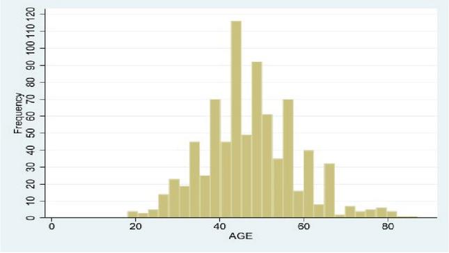
Figure 1 Histogram of the age of breast cancer patients.

The age distribution of breast cancer patients generally indicates that the highest incidence occurs among individuals aged 40 to 50 years, highlighting this group as the most frequently diagnosed. The data typically show a right-skewed distribution, with a gradual decrease in the number of diagnoses as age increases beyond 60 years. This distribution encompasses patients from their 20s to their 80s, though cases at the extremes of this age range are quite uncommon. Recognizing this demographic pattern is essential for effectively allocating healthcare resources and advancing research on breast cancer.

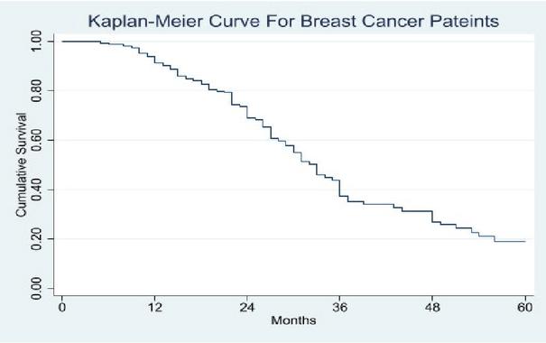
Figure 2 The overall Kaplan-Meier survival curve of breast cancer patients.

The Kaplan-Meier curve for breast cancer patients shows the cumulative survival rate over 60 months, with the Y-axis representing the proportion of patients still alive and the X-axis indicating time in months. Initially, the curve begins at 100% survival, reflecting that all patients were alive at the study’s start. However, there is a noticeable decline in survival rates during the first few months, suggesting a higher risk of mortality shortly after diagnosis or treatment initiation. Following this initial drop, the curve stabilizes, indicating a slower decline in survival rates, particularly after the 36-month mark. By the end of the 60 months, the cumulative survival rate has significantly decreased, underscoring that a substantial proportion of patients have not survived. This curve provides essential insights into the survival trends of breast cancer patients, highlighting critical periods where interventions may be vital for enhancing outcomes

Table 1 Demographic characteristics of breast cancer patients

Characteristics	Total	Percent	Characteristics	Total	Percent
Age groups			ALNM
$\le$50	510	63.6	Absent	241	30
$>$50	292	36.4	Present	561	70
Pathological Stages			Grades
Stage I	53	6.6	WD	62	7.7
Stage II	339	42.3	MD	369	46
Stage III	289	36	PD	371	46.3
Stage IV	121	15.1
Tumor			Metastasis
$<$2 cm	59	7.4	No	291	36.3
2 $<$ Tumor $\le$ 5 cm	385	48	Yes	511	63.7
$>$5 cm	358	44.6
*WD $=$ Well Differentiated, MD $=$ Moderately Differentiated, PD $=$ Poorly Differentiated.

The above data outlines various characteristics of breast cancer patients, categorized by age, axillary lymph node metastasis (ALNM), pathological stage, tumor grade, tumor size, and metastasis status. Among the age categories, 63.6% of patients are aged 50 or younger, while 36.4% are aged 50 or older. In terms of ALNM, 30% of patients do not exhibit lymph node involvement, whereas 70% do. Regarding pathological stages, the largest group of patients falls into Stage II (42.3%), followed by Stage III (36%), Stage IV (15.1%), and Stage I (6.6%). Analysing tumor grades, moderate differentiation (MD) and poorly differentiated (PD) tumors each account for about 46%, while well-differentiated (WD) tumours account for 7.7%. For tumor sizes, 48% are between 2 to 5 cm, 44.6% exceed 5 cm, and 7.4% are smaller than 2 cm. Finally, 63.7% of patients present with metastasis, indicating a significant portion of advanced disease. This detailed overview provides important insights into the demographic and clinical profiles of the patient population, which is essential for guiding treatment approaches and understanding outcomes.

Table 2 Results of goodness of fit of AFT model

AFT Model	Log-likelihood	AIC	BIC
Exponential	$-$316.9707	647.9415	680.7513
Weibull	$-$258.6639	533.3278	570.8247
Lognormal	$-$243.9687	503.9375	541.4344
Log-logistic	$-$243.90432	503.8086	541.3055

The evaluation of the Log-logistic model within the Accelerated Failure Time (AFT) framework shows promising results. It achieves a log-likelihood of $-$243.90432, indicating a strong fit to the data, slightly better than the Weibull model but just below the Lognormal model. The Log-logistic model also has an AIC of 503.8086, which is among the lowest in the comparison, suggesting it effectively balances fit and model complexity. Additionally, its BIC score of 541.3055 further supports its adequacy, as lower values indicate a preferable model. Overall, the Log-logistic model is a competitive option for analyzing the dataset, demonstrating strong performance in capturing the underlying survival patterns.

Table 3 Results of Log-logistic AFT model

		Standard		Time		95%	95%
Covariates	$\beta$	Error	z	Ratio	P value	LCI	UCI
Intercept	4.665	0.195	23.980	106.157	0.000	4.284	5.046
Age Groups	-0.001	0.076	-0.010	0.999	0.993	-0.150	0.148
Stages	-0.828	0.198	-4.170	0.437	0.000	-1.217	-0.439
Tumor	-0.230	0.095	-2.420	0.795	0.016	-0.416	-0.043
ALNM	0.120	0.158	0.760	1.127	0.448	-0.190	0.430
Grades	-0.115	0.101	-1.130	0.891	0.257	-0.313	0.084
Metastasis	-0.494	0.157	-3.150	0.610	0.002	-0.801	-0.186

The Table 3 summarises the findings from a regression analysis evaluating the impact of various covariates on the outcome. The intercept has a coefficient $(\beta )$ of 4.665 and a highly significant P value of 0.000, indicating a strong baseline effect. Among the covariates, Stages shows a significant negative association $(\beta =-0.828,\mathrm{P}=0.000)$, suggesting that advanced stages are associated with shorter survival. The Tumor variable also shows a negative association ($\beta =-0.230,\mathrm{P}=0.016$), while Metastasis shows a negative association $(\beta =-0.494,\mathrm{P}=0.002)$, both underscoring significant risks. In contrast, Age Groups, ALNM, and Grades do not exhibit statistically significant effects, with P values of 0.993, 0.448, and 0.257, respectively. The confidence intervals for these estimates highlight the uncertainty surrounding the non-significant covariates, while the significant ones clearly demonstrate their association with survival outcomes.

A substantial proportion of observations (approximately 80%) were right-censored in the present study. This high censoring rate is primarily attributable to patients who remained alive at the end of the study period or whose complete event information was unavailable during follow-up. Although survival analysis techniques are specifically designed to accommodate censored observations, a high level of censoring may reduce the precision of survival estimates and increase the variability of model parameter estimates. Consequently, the estimated survival probabilities and covariate effects should be interpreted with caution, particularly for longer follow-up durations. Nevertheless, the sample size of 802 patients provided sufficient information for reliable estimation of the fitted survival models.

Four parametric accelerated failure time models, namely the exponential, Weibull, lognormal, and log-logistic models, were compared using AIC and BIC criteria. The selected model demonstrated the best balance between goodness-of-fit and model complexity among the candidate models. However, model selection based solely on information criteria does not guarantee optimal predictive performance in external populations. Therefore, further validation using independent datasets or resampling-based approaches would be valuable for assessing the generalizability of the findings.

Model selection was performed using the Akaike Information Criterion (AIC) and Bayesian Information Criterion (BIC), which are widely accepted measures for balancing model fit and complexity. However, no external validation, cross-validation, or bootstrap-based assessment was conducted to evaluate the predictive performance and potential overfitting of the selected model. Therefore, the generalizability of the findings to other patient populations should be interpreted cautiously. Future studies may incorporate validation procedures to assess the robustness of the selected survival model.

This study has several limitations. First, the analysis was based on data obtained from a single hospital, which may limit the generalizability of the findings. Second, approximately 80% of observations were censored, potentially affecting the precision of survival estimates and parameter estimation. Third, although model selection was performed using established information criteria (AIC and BIC), no external validation, cross-validation, or bootstrap-based validation was conducted to evaluate potential overfitting and predictive performance.

4 Conclusion

Accelerated Failure Time (AFT) models are widely utilized in medical research for the parametric analysis of survival data. In this study, we employed four parametric AFT models: Exponential, Weibull, Lognormal, and Log-logistic, with the Log-logistic model demonstrating the best fit. The analysis shows that the effect of age on time-to-event is minimal, as indicated by a time ratio near 1 and a high p-value of 0.997 , suggesting that age does not significantly affect the timing of the event. Patients diagnosed with Stage III or IV cancer experience a significantly shorter time to event than those in earlier stages, reflected in a time ratio of 0.435, corresponding to a 56.5% reduction in time to event. This is statistically significant, highlighting the relevance of cancer stage as a predictor. Furthermore, larger tumors ($>$5 cm) are associated with shorter time to event, as evidenced by a time ratio of 0.803 and a p-value of 0.021, indicating a significant negative effect of tumour size on survival. In contrast, histologic grade does not have a statistically significant impact on time-to-event $(\mathrm{p}=0.236)$, as the time ratio suggests only a minor reduction in time for poorly differentiated tumors, which is insufficient for definitive conclusions. The presence of axillary lymph node metastasis does not significantly affect time-to-event $(\mathrm{p}=0.439)$, with the time ratio suggesting a slight increase in time-to-event that is not statistically significant. Conversely, metastasis is strongly associated with reduced time to event, as indicated by a time ratio of 0.611, corresponding to a 38.9% decrease in time, and is a significant factor in survival analysis. Family history also does not show a significant effect on time-to-event $(\mathrm{p}=0.321)$, with the time ratio indicating a minor decrease that is not statistically relevant. In conclusion, the log-logistic AFT model reveals that cancer stage, tumor size, and metastasis status significantly influence time-toevent outcomes. Conversely, age, histologic grade, axillary lymph node metastasis, and family history do not show significant associations. These results emphasize the importance of tumour characteristics and disease stage in predicting survival.

Acknowledgement

We are thankful to the State Cancer Institute in Guwahati and the North-East Cancer Hospital and Research Institute in Jorabat, Assam, for providing us with the breast cancer dataset.

Conflict of Interests

The authors declare that there is no conflict of interest.

References

Collett, D. (2023). Modelling survival data in medical research. Chapman and Hall/CRC.

Akaike, H. (1974). A new look at the statistical model identification. IEEE Transactions on Automatic Control, 19(6), 716–723.

Hosmer Jr, D. W., Lemeshow, S., and May, S. (2008). Applied survival analysis: regression modeling of time-to-event data. John Wiley & Sons.

Meiza, A., Awaluddin, A. S., Hidayah, N. O., and Taha, A. (2022). Comparison of different underlying distributions in the accelerated failure time (AFT) model on mortality of COVID-19 patients. InPrime: Indonesian Journal of Pure and Applied Mathematics, 4(2), 141–150.

Crowther, M. J., Royston, P., and Clements, M. (2023). A flexible parametric accelerated failure time model and the extension to time-dependent acceleration factors. Biostatistics, 24(3), 811–831.

Senyefia, B. A., Joseph, A., Cynthia, N. C., and Ouerfelli, N. (2022). A comparison between accelerated failure time models in analyzing the survival of breast cancer patients. J Cancer Tumor Int, 12(1), 16–28.

Wei, L. J. (1992). The accelerated failure time model: a useful alternative to the Cox regression model in survival analysis. Statistics in medicine, 11(14–15), 1871–1879.

Montaseri, M., Charati, J. Y., and Espahbodi, F. (2016). Application of parametric models to a survival analysis of hemodialysispatients. Nephro-urology monthly, 8(6), e28738.

Kleinbaum, D. G., and Klein, M. (1996). Survival analysis a self-learning text. Springer.

Khan, S. A., and Basharat, N. (2022). Accelerated failure time models for recurrent event data analysis and joint modeling. Computational Statistics, 37(4), 1569–1597.

Barman, R. S. M. P. (2017). Comparing accelerated failure time models with its specifi distributionsin theanalysis of esophagus cancer patients data. International Journal of Computational and Applied Mathematics, 12(2), 411–424.

Schwarz, G. (1978). Estimating the dimension of a model. The annals of statistics, 461–464.

Karimi, A., Delpisheh, A., and Sayehmiri, K. (2016). Application of accelerated failure time models for breast cancer patients’ survival in Kurdistan Province of Iran. Journal of Cancer Research and Therapeutics, 12(3), 1184–1188.

Swindell, W. R. (2009). Accelerated failure time models provide a useful statistical framework for aging research. Experimental gerontology, 44(3), 190–200.

Machin, D., Cheung, Y. B., and Parmar, M. (2006). Survival analysis: a practical approach. John Wiley & Sons.

Tripathy, M. R., Swain, P. K., Sarangi, P. K., and Pattnaik, S. S. (2022). Accelerated failure time models with applications to endometrial cancer survival data. Journal of Reliability and Statistical Studies, 723–744.

Anney, A. S., and Biswas, S. C. (2021). Under-5 Child Mortality Determinants in Rural-Urban Areas of Bangladesh: Proportional Hazard Models. Journal of Reliability and Statistical Studies, 121–140.

Biographies

Swapan Bhattacharjee received the master’s degree in Statistics from Cotton University in 2017. He is currently working as an Assistant Professor in the Department of Statistics at Tangla College, Tangla. He has more than 8 years of teaching experience and has published research papers in reputable journals and presented his research at national and international conferences. His research areas include medical research and population research.

Surobhi Deka serves as an Assistant Professor in the Department of Statistics at Cotton University, Guwahati, Assam, India. She holds a PhD from Tezpur University, where her doctoral research focused on statistical modeling of climate variables in the North East Region of India. Her expertise lies in applied statistics, with particular emphasis on extreme value distributions and survival analysis. She has authored numerous research papers published in refereed journals, successfully led a DST-funded project on flood hazard modeling under the Women Scientists Scheme, and actively contributes to the academic community as a reviewer for several international journals.

Journal of Reliability and Statistical Studies, Vol. 19, Issue 2 (2026), 717–732
doi: 10.13052/jrss0974-8024.19219
© 2026 River Publishers