The Unit Omega Distribution as an Alternative to the Beta Distribution for the Modeling to the Infrared Thermography Temperature Data

Alia A. Alkhathami¹, Mahfooz Alam^2,*, Aafaq A. Rather³, Mehdi Hosseinzadeh^{4, 5} and Showkat Ahmad Lone¹

¹Department of Basic Science, College of Science and Theoretical Studies, Saudi Electronic University, Riyadh 11673, Kingdom of Saudi Arabia
²Department of Mathematics and Statistics, Faculty of Science and Technology, Vishwakarma University, Pune-411 048, India
³Symbiosis Statistical Institute, Symbiosis International (Deemed University), Pune, India
⁴Department of AI, School of Computer Science and Engineering, Galgotias University, Greater Noida, India
⁵International Center for Materials Sciences and Technology, Western Caspian University, Baku, Azerbaijan
E-mail: mahfooz.stats@gmail.com; aafaq7741@gmail.com; mehdihosseinzadeh@duytan.edu.vn
*Corresponding Author

Received 10 March 2026; Accepted 01 July 2026

Abstract

Proportion data is significant in many disciplines, including as economics, finance, reliability engineering, medicine, biology, and chemistry, since it serves as the basis for identifying trends, expediting procedures, and making well-informed conclusions that result in advances and innovations. For the representation and analysis of proportional data, the beta distribution is a standard model. In this paper, we explore the unit omega distribution [15] and their ordered properties such as the exact expressions, as well as recurrence relations, for the single moments of the order statistics (OSs) and record values. Additionally, various L-moment characteristics based on OS moments and record values were analyzed. The applicability of the unit omega distribution over beta distribution was demonstrated through its successful fit to the original IRT temperature dataset. For comparative assessment, the performance of the unit omega distribution was evaluated against the commonly used beta distribution using the Kolmogorov–Smirnov (KS) goodness-of-fit test. The results indicate that the unit omega distribution yields a smaller KS test statistic and a larger associated p-value compared to the Beta distribution, suggesting a superior fit to the observed data. These findings highlight the flexibility and effectiveness of the unit omega distribution in modelling bounded data. Furthermore, the study provides a strong foundation for future research, particularly in extending the analysis to generalized order statistics and progressive censoring schemes associated with the unit omega distribution.

Keywords: Order statistics, record values, moments, L-moments, recurrence relations, hypergeometric function, absolute Stirling number, infrared thermography temperature.

1 Introduction

Many different fields, such as economics, finance, reliability engineering, medicine, biology, and chemistry, deal with proportion data. A random variable is considered proportion data if its values fall inside the unit interval [0,1] and are represented as a fraction or percentage of a whole. Effective modeling requires specific probability distributions to describe the patterns and variations within this constrained range. Applications in fields like acceptance rates, recovery and mortality rates, test scores, and other proportional indicators in healthcare and education highlight the importance of these models. The development of distributions appropriate for bounded intervals has been the subject of significant research efforts throughout the last ten years. Random variable transformations, function compositions, and the creation of new distributions are methods for creating these models.

One well-known example of a bounded distribution is the beta distribution [27], which is used extensively in many different scientific fields and is distinguished by its versatility in density forms. Several alternative distributions have been suggested in the statistical literature to increase modeling accuracy on the bounded interval $[0,1]$. Among them, two well-known instances of unit distributions that have attracted a lot of interest in the applied sciences are the Topp-Leone distribution (first shown by Topp and Leone in 1955) and the Kumaraswamy distribution (first presented by Kumaraswamy in 1980). Despite their widespread use, these distributions are less theoretically tractable due to the absence of closed-form equations for moments. New families of unit distributions have been introduced in recent study in response to the growing interest in bounded distributions. These consist of the unit-Lindley distribution (Mazucheli et al., [36]), unit-bimodal (Martínez-Flórez et al., [32]), unit-inverse Gaussian (Ghitany et al., [23]), unit Weibull (Mazucheli et al.,[35]), unit log-logistic (Ribeiro-Reis, [42]), unit Muth (Maya et al., [34]), and the unit generalized half-normal distribution (Korkmaz [30]).

1.1 The Unit Omega Probability Distribution

The Omega distribution was first presented by Dombi et al. [20]. It is represented by the equation $\text{Omg}(\alpha ,\beta ,d)$ and has three positive parameters ($\alpha ,\beta ,d$). The probability density function (pdf) and cumulative distribution function (cdf) can be give as

$$f(x)=\alpha \beta d^{2\beta }{x}^{\beta -1}\frac{1}{d^{2\beta }-x^{2\beta }}{\left(\frac{d^{\beta }+x^{\beta }}{d^{\beta }-x^{\beta }}\right)}^{-\frac{\alpha d^{\beta }}{2}},\text{if}0<x<d,$$

and

$$F(x)=1-{\left(\frac{d^{\beta }+x^{\beta }}{d^{\beta }-x^{\beta }}\right)}^{-\frac{\alpha d^{\beta }}{2}},\text{if}0<x<d,$$

respectively.

Studies by Okorie and Nadarajah [39], Alsubie et al. [10], Jónás and Bakouch [28], and Özbilén and Genç [40] provide more information and discussions on the Omega distribution. In particular, the Omega distribution is supported on the unit interval and reduces to the unit Omega distribution for d=1. The density and distribution functions are analyzed in Birbiçer and Genç [15], Prataviera and Cordeiro [41] for further details on this case. The probability density function ($pdf$) and cumulative distribution function ($cdf$) can be give as

$$f(x)=\alpha \beta x^{\beta -1}\frac{1}{1-x^{2\beta }}{\left(\frac{1+x^{\beta }}{1-x^{\beta }}\right)}^{-\frac{\alpha }{2}},\text{if}0<x<1,$$

(1)

and

$$F(x)=1-{\left(\frac{1+x^{\beta }}{1-x^{\beta }}\right)}^{-\frac{\alpha }{2}},\text{if}0<x<1,$$

(2)

respectively.

From now on, a random variable with density (1) is represented by $X$. Observe that

$$(1-x^{2\beta })f(x)=\alpha \beta x^{\beta -1}[1-F(x)].$$

(3)

Several authors, including Malik et al. [31], Balakrishnan et al. [13], and Balakrishnan and Sultan [14], have constructed recurrence relations for single and product moments of order statistics for particular distributions. In statistical literature, the uses of moments of order statistics are widely recognized. For instance, they are helpful in nonparametric statistics, statistical modeling, statistical inferences, and decision-making processes, among other areas.

Explicit expressions for moments of order statistics of some distributions were determined by Nadarajah [37]. For more results in this context, one may also refer to Nagaraja [38], Çetinkaya and Genç [17], Alam et al. [7] Almuhayfith et al. [8] and Singh et al. [43] references therein.

On the other hand, we obtain the precise expressions for the moments of these quantities that disclose some significant features of the unit Omega distribution because of the numerous applications of the order statistics (OSs) and the record values. Specifically, we identify important components of the information theory as an entropy measure of the record values and OSs. It is necessary to recall some mathematical background in order to make these contributions more accurate.

In practice, the aforementioned ideas are crucial. Extreme OSs and record values, such as weather (hottest day, coolest day, flood levels) in a decade, economic conditions in a year, sports (highest jump, minimum time to complete swimming, etc.), industrial stress testing (minimum and maximum time to failure), seismology, mining surveys, shock models, reliability testing, and meteorological data analysis are examples of data that are occasionally more specific by the order random variable. Forecasting future record values, such as the next earthquake’s magnitude, the greatest (record) level of water dam hold or release, and the market index’s extreme point, is crucial.. For more applications, see [4, 5, 6] etc.

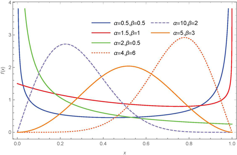
Figure 1 Behaviour of the unit Omega distribution (U-shaped, reverse J-shaped, J-shaped, increasing-decreasing increasing-shaped, unimodal and left and right-skewed distribution) at different values of different parameters.

The rest of the paper is organized as follows: In Section 2, derive the supporting results in form of lemmas which are used in the subsequent sections. The precise formulas and recurrence relations for OSs’ single and product moments are found in Section 3. The precise formulations and a recurrence relation for single moments are derived from record values in Section 4. The L-moments of estimation of the unit omega distribution is presented in Section 5 and is successfully applied to an original IRT temperature dataset. The study is finally over, and Section 6 discusses future work.

2 Supporting Results

The following lemma is needed to calculate OSs’ and record moments from the unit Omega distribution.

Lemma 1 (See, Gradshteyn and Ryzhik [24] and Mathai and Saxena [33])

We have

${\displaystyle {\int }_0^1}{x}^{\lambda -1}{(1-x)}^{\mu -1}{(1-\eta x)}^{-\nu }\mathit{d}x$

$=B(\lambda ,\nu ){}_2{}^{}F_1^{}(\nu ,\lambda ;\lambda +\mu ;\eta ),\lambda >0,\mu >0,$

where $B(\lambda ,\nu )$ beta function and ${}_2{}^{}F_1^{}(a,b;c;x)$ denote the Gauss hypergeometric function defined by

$B(a,b)={\displaystyle {\int }_0^1}{t}^{a-1}{(1-t)}^{b-1}\mathit{d}t\text{and}{}_2{}^{}F_1^{}(a,b;c;x)={\displaystyle \sum _{i=0}^{\mathrm{\infty }}}{\displaystyle \frac{{(a)}_i{(b)}_i}{{(c)}_i}}{\displaystyle \frac{x^i}{i!}},$

where ${(p)}_i=p(p+1)\mathrm{\dots }(p+i-1)=\frac{\mathrm{\Gamma }(p+i)}{\mathrm{\Gamma }(p)}$ denotes the ascending factorial.

The hypergeometric function [see, Mathai and Saxena [33]] can be also written as

$${}_p{}^{}F_q^{}[a_1,\mathrm{\dots },a_p;b_1,\mathrm{\dots },b_q;x]=\sum _{r=0}^{\mathrm{\infty }}\left[\prod _{j=1}^p\frac{\mathrm{\Gamma }(a_j+r)}{\mathrm{\Gamma }(a_j)}\right]\left[\prod _{j=1}^q\frac{\mathrm{\Gamma }(b_j)}{\mathrm{\Gamma }(b_j+r)}\right]\frac{x^r}{r!}.$$

For the convergence: The series ${}_{\mathrm{p}}{}^{}\mathrm{F}_{\mathrm{q}}^{}[{\mathrm{a}}_1,\mathrm{\dots },{\mathrm{a}}_{\mathrm{p}};{\mathrm{b}}_1,\mathrm{\dots },{\mathrm{b}}_{\mathrm{q}};\mathrm{x}]$ converges for $|\mathrm{x}|<1$, diverges for $|\mathrm{x}|>1$ and for $|\mathrm{x}|=1$, ${}_{\mathrm{p}}{}^{}\mathrm{F}_{\mathrm{q}}^{}$ converges only for $\mathrm{p}=\mathrm{q}+1$ and ${\sum }_{\mathrm{j}=1}^{\mathrm{q}}{\mathrm{b}}_{\mathrm{j}}-{\sum }_{\mathrm{j}=1}^{\mathrm{p}}{\mathrm{a}}_{\mathrm{j}}>0$.

At $p=2$ and $q=1$, this ${}_2{}^{}F_1^{}(a,b;c;x)$ is known as Gauss hypergeometric series, which is defined above.

Lemma 2 For the unit Omega distribution given in (1), $a$ and $k$ are non negative finite integers, we have,

${\mathrm{\Phi }}_{\alpha ,\beta }^k(a)$	$=\alpha B({\displaystyle \frac{k}{\beta }}+1,{\displaystyle \frac{\alpha (a+1)}{2}}+1)$
	${\times }_2{F}_1({\displaystyle \frac{\alpha (a+1)}{2}}+1,{\displaystyle \frac{k}{\beta }}+1;{\displaystyle \frac{k}{\beta }}+{\displaystyle \frac{\alpha (a+1)}{2}}+1;-1).$	(4)
${\mathrm{\Phi }}_{\alpha ,\beta }^k(0)$	$=\alpha B({\displaystyle \frac{k}{\beta }}+1,{\displaystyle \frac{\alpha }{2}}+1)$
	${\times }_2{F}_1({\displaystyle \frac{\alpha }{2}}+1,{\displaystyle \frac{k}{\beta }}+1;{\displaystyle \frac{k}{\beta }}+{\displaystyle \frac{\alpha }{2}}+1;-1).$	(5)

where

$${\mathrm{\Phi }}_{\alpha ,\beta }^k(a)={\int }_0^1{x}^k{[1-F(x)]}^{a}f(x)\mathit{d}x$$

(6)

Proof. In view of (6), we can write

$${\mathrm{\Phi }}_{\alpha ,\beta }^k(a)={\int }_0^1{x}^k{[1-F(x)]}^{a+1}\frac{f(x)}{[1-F(x)]}\mathit{d}x$$

from (3), and the result can be seen as

${\mathrm{\Phi }}_{\alpha ,\beta }^k(a)$	$=\alpha \beta {\displaystyle {\int }_0^1}{\displaystyle \frac{x^{k+\beta -1}}{(1-x^{2\beta })}}{[1-F(x)]}^{a+1}\mathit{d}x.$
	$=\alpha \beta {\displaystyle {\int }_0^1}{\displaystyle \frac{x^{k+\beta -1}}{(1+x^{\beta })(1-x^{\beta })}}{\left({\displaystyle \frac{1+x^{\beta }}{1-x^{\beta }}}\right)}^{-\frac{\alpha (a+1)}{2}}\mathit{d}x.$
	$=\alpha \beta {\displaystyle {\int }_0^1}{x}^{k+\beta -1}{(1-x^{\beta })}^{\frac{\alpha (a+1)}{2}-1}{(1+x^{\beta })}^{-\frac{\alpha (a+1)}{2}-1}\mathit{d}x.$	(7)

Setting $t=x^{\beta }$, (2) can be rewritten as

$${\mathrm{\Phi }}_{\alpha ,\beta }^k(a)=\alpha {\int }_0^1{t}^{k/\beta }{(1-t)}^{\frac{\alpha (a+1)}{2}-1}{(1+t)}^{-\frac{\alpha (a+1)}{2}-1}\mathit{d}t.$$

Using the integral formula as Lemma 1, we obtain

${\mathrm{\Phi }}_{\alpha ,\beta }^k(a)$	$=\alpha B({\displaystyle \frac{k}{\beta }}+1,{\displaystyle \frac{\alpha (a+1)}{2}}+1)$
	${\times }_2{F}_1({\displaystyle \frac{\alpha (a+1)}{2}}+1,{\displaystyle \frac{k}{\beta }}+1;{\displaystyle \frac{k}{\beta }}+{\displaystyle \frac{\alpha (a+1)}{2}}+1;-1).$

Inserting $a=0$ in the above equation, it follows (2) as the $k$-th moment of the unit Omega distribution.

The infinite series involved in Lemmas 1 and 2 serves as the foundation for the moment properties discussed in Section 3.1. In statistics, determining closed-form equations for computing moments of order statistics is a frequently researched subject. Although numerical calculations are possible for these functions, mathematical and statistical software programs like Python and R offer quick and easy computations. Therefore, a useful and convenient method for analysis is provided by the expressions derived in Section 3.1.

3 Moments of the Unit Omega Distribution Based on OSs

The Exact expressions and recurrence relations for the single moments of the unit omega distribution and related order statistics are presented in this section.

3.1 Relations for Single Moments

Order Statistics (OSs) are random variables ordered in terms of increasing magnitude. Suppose that $X_1,X_2,\mathrm{\dots },X_n$ are independent, identically distributed random variables with a cumulative distribution function (cdf) $F(x)$ and a probability density function (pdf) $f(x)$. Now let $X_{1:n}\le X_{2:n}\le \mathrm{\cdots }\le X_{n:n}$ stand for the OSs of $X_1,\mathrm{\dots },X_n$. For any $1\le r\le n$, the $r$th OS, $X_{r:n}$, provides the pdf $f_{r:n}(x)$ as follows:

$$f_{r:n}(x)=C_{r:n}{F}^{r-1}(x){[1-F(x)]}^{n-r}f(x),0\le x<\mathrm{\infty },$$

(8)

where

$$C_{r:n}=\frac{n!}{(r-1)!(n-r)!}.$$

Next, the $kth$ single moment of $X_{r:n}^k$ takes the form

$${\mu }_{r:n}^{(k)}=E(X_{r:n}^k)={\int }_0^d{x}^k{f}_{r:n}(x)\mathit{d}x;1\le r\le n;k\in \mathbb{N},$$

(9)

For basic information on order statistics (OSs), which tackle many theoretical and practical issues, see [9] and [19]. L-moments [26] and best linear unbiased estimation for location-scale families of distributions [12] are two examples of parameter estimation strategies. Additionally, OSs are used in goodness-of-fit assessments. [9] characterisations of probability distributions [3, 9, 19, 12]. Additionally, OSs are used to create a variety of statistics. The following theorem describes the moments related to $X_{r:n}$. By simply changing the values of $n$ and $r$, this theorem gives the precise moments and associated recurrence relations for the unit Omega distribution.

Theorem 1 The following formula is obtained for $1\le r\le n$ and $k\in \mathbb{N}$.

$${\mu }_{r:n}^{(k)}=C_{r:n}\sum _{i=0}^{r-1}{(-1)}^i\left(\genfrac{}{}{0pt}{}{r-1}{i}\right){\mathrm{\Phi }}_{\alpha ,\beta }^k(n-r+i)$$

(10)

or

${\mu }_{r:n}^{(k)}$	$=C_{r:n}\alpha {\displaystyle \sum _{i=0}^{r-1}}{(-1)}^i\left({\displaystyle \genfrac{}{}{0pt}{}{r-1}{i}}\right)B({\displaystyle \frac{k}{\beta }}+1,{\displaystyle \frac{\alpha }{2}}(i+n-r+1)+1)$
	${\times }_2{F}_1({\displaystyle \frac{\alpha }{2}}(i+n-r+1)+1,{\displaystyle \frac{k}{\beta }}+1;{\displaystyle \frac{k}{\beta }}$
	$+{\displaystyle \frac{\alpha }{2}}(i+n-r+1)+1;-1),$	(11)

where $C_{r:n}$ is defined as before.

Proof: From Equation (9), we have

${\mu }_{r:n}^{(k)}$	$=C_{r:n}{\displaystyle {\int }_0^1}{x}^k{[F(x)]}^{r-1}{[1-F(x)]}^{n-r}f(x)\mathit{d}x.$
	$=C_{r:n}{\displaystyle \sum _{i=0}^{r-1}}{(-1)}^i\left({\displaystyle \genfrac{}{}{0pt}{}{r-1}{i}}\right){\displaystyle {\int }_0^1}{x}^k{[1-F(x)]}^{n-r+i}f(x)\mathit{d}x.$	(12)

Applying the Lemma 2, we get the yield as results.

Remark 1 By setting $n=r=1$ in Theorem 1, we obtain

${\mu }_{1:1}^{(k)}=E(X^k)$	$=\alpha B({\displaystyle \frac{k}{\beta }}+1,{\displaystyle \frac{\alpha }{2}}+1)$
	${\times }_2{F}_1({\displaystyle \frac{\alpha }{2}}+1,{\displaystyle \frac{k}{\beta }}+1;{\displaystyle \frac{k}{\beta }}+{\displaystyle \frac{\alpha }{2}}+1;-1),$	(13)

which is the $kth$ moment of $X$ for the unit Omega distribution.

By substituting $k=1,2,3,$ and $4$ into Equation (1), the closed-form expressions for the first four moments of $X$ can be derived, along with its variance, skewness, and kurtosis.

Remark 2 For $r=1$ in Theorem 1,

${\mu }_{1:n}^{(k)}$	$=n\alpha B({\displaystyle \frac{k}{\beta }}+1,{\displaystyle \frac{n\alpha }{2}}+1)$
	${\times }_2{F}_1({\displaystyle \frac{n\alpha }{2}}+1,{\displaystyle \frac{k}{\beta }}+1;{\displaystyle \frac{k}{\beta }}+{\displaystyle \frac{n\alpha }{2}}+1;-1),$	(14)

and, for $r=n$ in Theorem 1,

${\mu }_{n:n}^{(k)}$	$=n\alpha {\displaystyle \sum _{i=0}^{n-1}}{(-1)}^i\left({\displaystyle \genfrac{}{}{0pt}{}{n-1}{i}}\right)B({\displaystyle \frac{k}{\beta }}+1,{\displaystyle \frac{\alpha }{2}}(i+1)+1)$
	${\times }_2{F}_1({\displaystyle \frac{\alpha }{2}}(i+1)+1,{\displaystyle \frac{k}{\beta }}+1;{\displaystyle \frac{k}{\beta }}+{\displaystyle \frac{\alpha }{2}}(i+1)+1;-1),$	(15)

which are the $kth$ moments of the minimum and the maximum order statistics, respectively.

Recurrence relations for single moments of order statistics from the $cdf$ (2) follow in the next theorem.

Theorem 2 For $1\le r\le n$ and $k\in \mathbb{N}$, we have

$${\mu }_{r:n}^{(k)}-{\mu }_{r-1:n-1}^{(k)}=\frac{k}{n\alpha \beta }\left[{\mu }_{r:n}^{(k-\beta )}-{\mu }_{r:n}^{(k+\beta )}\right]$$

(16)

and, consequently,

$${\mu }_{r:n}^{(k)}-{\mu }_{r-1:n}^{(k)}=\frac{k}{(n-r+1)\alpha \beta }\left[{\mu }_{r:n}^{(k-\beta )}-{\mu }_{r:n}^{(k+\beta )}\right].$$

(17)

Proof: Khan et al. [29] proved that (for $1\le r\le n$)

$${\mu }_{r:n}^{(k)}-{\mu }_{r-1:n-1}^{(k)}=\left(\genfrac{}{}{0pt}{}{n-1}{r-1}\right)k{\int }_0^{\mathrm{\infty }}{x}^{k-1}{[F(x)]}^{r-1}{[1-F(x)]}^{n-r+1}\mathit{d}x.$$

(18)

or, equivalently, from (3),

${\mu }_{r:n}^{(k)}-{\mu }_{r-1:n-1}^{(k)}$	$=\left({\displaystyle \genfrac{}{}{0pt}{}{n-1}{r-1}}\right){\displaystyle \frac{k}{\alpha \beta }}{\displaystyle {\int }_0^1}{x}^{k-\beta }{[F(x)]}^{r-1}{[1-F(x)]}^{n-r}f(x)\mathit{d}x$
	$+\left({\displaystyle \genfrac{}{}{0pt}{}{n-1}{r-1}}\right){\displaystyle \frac{k}{\alpha \beta }}{\displaystyle {\int }_0^1}{x}^{k+\beta }{[F(x)]}^{r-1}{[1-F(x)]}^{n-r}f(x)\mathit{d}x,$

which after simplification yields (16).

Using the well-known recurrence relation for moments that follows (David and Nagaraja, [19])

$$n{\mu }_{r:n-1}^{(k)}=(n-r){\mu }_{r:n}^{(k)}+r{\mu }_{r+1:n}^{(k)},$$

in Equation (16), we obtain (17).

Remark 3 By setting $k=1,\mathrm{\hspace{0.17em}2}$ in Theorem 1, we calculate the means, second moments of the order statistics for the Omega distribution (for $n=1(1)5$) and selected parameter values. The computed values to six decimal places are reported in Tables 1 and 2. It can be seen that the condition ${\sum }_{r=1}^n{\mu }_{r:n}=nE(X)$ holds (see David and Nagaraja, [19]).

The variance of $X_{r:n}$ ($1\le r\le n$) is $V(X_{r:n})={\mu }_{r:n}^{(2)}-{\left[{\mu }_{r:n}^{(1)}\right]}^2$, Remark where ${\mu }_{r:n}^{(1)}$ and ${\mu }_{r:n}^{(2)}$ can be calculated by setting $k=1$ and $k=2$ in Theorem 1, respectively. Using the Python software is to compute the means, second moments and variances.

Table 1 Means and variances of order statistics from the unit omega distribution

		$\alpha =0.25$, $\beta =0.75$			$\alpha =0.75$, $\beta =0.25$
$n$	r	${\mu }_{r:n}^{(1)}$	${\mu }_{r:n}^{(2)}$	$V[X_{r:n}]$	${\mu }_{r:n}^{(1)}$	${\mu }_{r:n}^{(2)}$	$V[X_{r:n}]$
1	1	0.041911	0.025105	0.023348	0.028264	0.012551	0.011752
2	1	0.066990	0.037790	0.033302	0.024767	0.008797	0.008184
	2	0.016832	0.012419	0.012136	0.031762	0.016306	0.015297
3	1	0.081761	0.043467	0.036782	0.018108	0.005153	0.004825
	2	0.037448	0.026435	0.025033	0.038085	0.016083	0.014633
	3	0.006525	0.005412	0.005369	0.028601	0.016418	0.015600
4	1	0.006525	0.005412	0.005369	0.012763	0.002919	0.002756
	2	0.056823	0.038362	0.035133	0.034142	0.011858	0.010692
	3	0.018072	0.014508	0.014181	0.042027	0.020308	0.018542
	4	0.002675	0.002380	0.002373	0.024125	0.015121	0.014539
5	1	0.094273	0.044636	0.035749	0.008996	0.001659	0.001578
	2	0.073272	0.047299	0.041930	0.027832	0.007958	0.007183
	3	0.032151	0.024956	0.023922	0.043607	0.017707	0.015805
	4	0.008687	0.007543	0.007468	0.040973	0.022042	0.020363
	5	0.001173	0.001089	0.001088	0.019913	0.013391	0.012994

Table 2 Means and variances of order statistics from the unit omega distribution

		$\alpha =0.50$, $\beta =1.50$			$\alpha =1.50$, $\beta =0.50$
$n$	r	${\mu }_{r:n}^{(1)}$	${\mu }_{r:n}^{(2)}$	$V[X_{r:n}]$	${\mu }_{r:n}^{(1)}$	${\mu }_{r:n}^{(2)}$	$V[X_{r:n}]$
1	1	0.103031	0.066990	0.056375	0.061254	0.024767	0.021015
2	1	0.151234	0.090073	0.067201	0.045722	0.012763	0.010672
	2	0.054828	0.043906	0.040900	0.076786	0.036770	0.030874
3	1	0.174497	0.095830	0.065381	0.032223	0.006417	0.005379
	2	0.104709	0.078559	0.067595	0.072720	0.025455	0.020167
	3	0.029887	0.026580	0.025687	0.078819	0.042428	0.036216
4	1	0.185326	0.094443	0.060097	0.023351	0.003429	0.002884
	2	0.142009	0.099993	0.079826	0.058842	0.015381	0.011919
	3	0.067409	0.057124	0.052580	0.086599	0.035529	0.028030
	4	0.017379	0.016399	0.016097	0.076225	0.044728	0.038918
5	1	0.189559	0.090161	0.054228	0.017530	0.001957	0.001650
	2	0.168393	0.111569	0.083213	0.046632	0.009318	0.007143
	3	0.102432	0.082629	0.072137	0.077156	0.024474	0.018521
	4	0.044061	0.040121	0.038180	0.092894	0.042900	0.034271
	5	0.010709	0.010468	0.010353	0.072058	0.045185	0.039993

4 Moments of the Unit Omega Distribution Based on Record Values

In this section, we derive the exact expression for the single moments of upper record values from the unit Omega distribution, noting that the marginal pdf of the $n$th upper record value is defined in Equation (19).

Record values (or simply records) are defined as random variables that exceed all previously observed values in a sequence. Let $n$ be a positive integer, and consider a sequence of $n$ independent and identically distributed random variables $X_1,X_2,\mathrm{\cdots },X_n$ with cumulative distribution function F(x) and probability density function pdf. Define $Y_n=\max (\min )\{X_1,X_2,\mathrm{\cdots },X_n\}$ for $n\ge 1.$ We say $X_j$ is a lower(upper) record value of this sequence if $Y_j<(>)Y_{j-1}$ for $j>1$. By definition, $X_1$ is a lower as well as an upper record value. Let $U(n)=\min \{j|j>U(n-1),Y_j>Y_{U(n-1)},n\ge 2\}$, with $U(1)=1$ denoting the times of upper record values. Similarly, let $L(n)=\min \{j|j>L(n-1),Y_j<Y_{L(n-1)},n\ge 2\}$, with $L(1)=1$ denoting the times of lower record values. Then $X_{L(n)}$ and $X_{U(n)}$ are the $n$th lower and upper record values, respectively. The concept of record values was coined by [16]. For a survey on important results in this area, one may refer to [1, 2] and [11].

The marginal pdf of the $n$th upper record value is given as

$f_{X_{U(n)}}(x)={\displaystyle \frac{1}{(n-1)!}}{[-\ln \overline{F}(x)]}^{n-1}f(x),-\mathrm{\infty }<x<\mathrm{\infty }.$

(19)

By the same analogous, we define the marginal $pdf$ of the $n$th upper record value replacing $F(.)$ by $1-F(.)$ in Equation $(\text{19})$. Next, the $kth$ single moment of $X_{U(n)}$ takes the form

$E[X_{U(n)}^k]={\displaystyle {\int }_0^1}{x}^k{f}_{X_{U(n)}}(x)\mathit{d}x;k\in \mathbb{N},$

(20)

Theorem 3 Let $k\in \mathbb{N}$ Then, in the context of the unit Omega distribution $(\text{1})$, we get

$$E[X_{U(n)}^k]=\sum _{a=n-1}^{\mathrm{\infty }}\sum _{b=0}^a{(-1)}^b\left(\genfrac{}{}{0pt}{}{a}{b}\right)\frac{c(a,n-1)}{a!}{\mathrm{\Phi }}_{\alpha ,\beta }^k(b),$$

(21)

where ${\mathrm{\Phi }}_{\alpha ,\beta }^k(a)$ is defined by Equation $(\text{2})$.

Proof. From Equation $(\text{19})$ and (20), we have

$$E[X_{U(n)}^k]=\frac{1}{(n-1)!}{\int }_0^1{x}^k{[-\ln \overline{F}(x)]}^{n-1}f(x)\mathit{d}x.$$

(22)

For any real number $r$ and $|x|<1$, we have Comtet [18]

$${[-\ln (1-x)]}^r=r!\sum _{p\ge r}\frac{c(p,r)}{p!}{x}^p,$$

(23)

where $c(p,r)$ is the number of permutations of $p$ elements with $r$ cycles (absolute Stirling numbers), hence $c(p,r)=0$ if not $1\le r\le p$ except $c(0,0)=1$. On substituting (23) in (22). Therefore, we have

$$E[X_{U(n)}^k]=\sum _{a=n-1}^{\mathrm{\infty }}\frac{c(a,n-1)}{a!}{\int }_0^1{x}^k{[1-\overline{F}(x)]}^{a}f(x)\mathit{d}x.$$

Thus, by using the binomial expansion and Lemma 2, we get

$$E[X_{U(n)}^k]=\sum _{a=n-1}^{\mathrm{\infty }}\sum _{b=0}^a{(-1)}^b\left(\genfrac{}{}{0pt}{}{a}{b}\right)\frac{c(a,n-1)}{a!}{\mathrm{\Phi }}_{\alpha ,\beta }^k(b).$$

This completes the proof of the theorem.

Tables 3 and 4 explain the moments of the upper record values when $\beta$ is fixed $0.50$ and $1.50$ respectively and varying the $\alpha$ and $n=1(1)7$ from the unit Omega distribution.

Table 3 The values of $E[X_{U(n)}]$ associated with the unit omega distribution at different parameters

	$\beta =0.50$
$\alpha /n$	1	2	3	4	5	6	7
0.25	0.036830	0.009385	0.003052	0.001204	0.000557	0.000295	0.000175
0.50	0.057338	0.026043	0.014631	0.009630	0.007170	0.005893	0.005250
0.75	0.068115	0.041410	0.030316	0.025328	0.023365	0.023280	0.024665
1.00	0.073009	0.053114	0.045554	0.043749	0.045638	0.050709	0.059210
1.25	0.074328	0.061087	0.058208	0.061245	0.069194	0.082479	0.102507
1.50	0.073486	0.065955	0.067726	0.075987	0.090776	0.113638	0.147504
1.75	0.071368	0.068445	0.074306	0.087421	0.108814	0.141213	0.189245
2.00	0.068528	0.069197	0.078413	0.095668	0.122876	0.163907	0.225079
2.25	0.065318	0.068721	0.080557	0.101140	0.133149	0.181490	0.254048
2.50	0.061960	0.067400	0.081202	0.104328	0.140100	0.194312	0.276221
2.75	0.058595	0.065521	0.080735	0.105708	0.144280	0.202977	0.292207
3.00	0.055306	0.063290	0.079463	0.105694	0.146225	0.208163	0.302840

Table 4 The values of $E[X_{U(n)}]$ from the unit omega distribution at different parameters

	$\beta =1.50$
$\alpha /n$	1	2	3	4	5	6	7
0.25	0.077910	0.014341	0.003925	0.001402	0.000611	0.000312	0.000181
0.50	0.130349	0.042456	0.019954	0.011817	0.008238	0.006490	0.005622
0.75	0.166049	0.072124	0.044016	0.032941	0.028306	0.026885	0.027549
1.00	0.190445	0.098812	0.070486	0.060443	0.058503	0.061704	0.069387
1.25	0.207035	0.121261	0.095960	0.089935	0.093994	0.106007	0.126464
1.50	0.218140	0.139500	0.118850	0.118561	0.130717	0.154430	0.191911
1.75	0.225334	0.154008	0.138627	0.144810	0.166047	0.202949	0.259842
2.00	0.229710	0.165366	0.155301	0.168050	0.198550	0.249032	0.326158
2.25	0.232036	0.174130	0.169119	0.188158	0.227593	0.291306	0.388368
2.50	0.232863	0.180783	0.180422	0.205275	0.253031	0.329179	0.445166
2.75	0.232591	0.185730	0.189559	0.219667	0.274991	0.362543	0.496041
3.00	0.231510	0.189302	0.196858	0.231642	0.293736	0.391566	0.540973

5 Applications

The characteristics of L-moments for the unit omega distribution, such as the L-coefficient of variation, measures of variability, L-skewness, and L-kurtosis, are examined in this section. In addition, we used order statistics (OSs) from Infrared Thermography (IRT) temperature data, which were previously examined by Wang et al. [44], to fit the unit omega distribution. Using the L-moments of the OSs, the parameters of the unit omega distribution are computed. Lastly, we investigate the connections between the record values.

5.1 L-Moments

L-moments provide greater robustness against outliers compared to traditional moments and exhibit minimal sample variance. Beyond summarizing observed data, they are instrumental in characterizing probability distributions for model specification, “parameter estimation, and hypothesis testing. L-moments are defined as the expectations of specific linear combinations of order statistics Hosking [26]. For any $m\ge 1$, the $m$th L-moment of a distribution is expressed as:

$$L_m=\frac{1}{m}\sum _{j=0}^{m-1}{(-1)}^j\left(\genfrac{}{}{0pt}{}{m-1}{j}\right){\mu }_{m-j:m},$$

(24)

The first four L-moments are $L_1={\mu }_{1:1},$ $L_2=\frac{1}{2}\left[{\mu }_{2:2}-{\mu }_{1:2}\right],$ $L_3=\frac{1}{3}\left[{\mu }_{3:3}-2{\mu }_{2:3}+{\mu }_{1:3}\right],$ and $L_4=\frac{1}{4}\left[{\mu }_{4:4}-3{\mu }_{3:4}+3{\mu }_{2:4}-{\mu }_{1:4}\right],$ respectively. L-moments are directly analogous to conventional moments, such as mean, variance, skewness, kurtosis, and so on. The properties and applications of L-moments were much explored by [26], which contain L-coefficient of variation (L-CV), which is a dimensionless measure of variability and defined by $L_2/L_1,$ and L-skewness and L-kurtosis, which are dimensionless measures of asymmetry and kurtosis, respectively, defined by ${\tau }_3=L_3/L_2$ and ${\tau }_4=L_4/L_2$.

For $m=1,2$ in (24), the first and second L-moments are given as

$L_1=E(X_{1:1})\text{and}{L}_2={\displaystyle \frac{1}{2}}E(X_{2:2}-X_{1:2}).$

(25)

As per Hosking and Wallis [25], the first and second sample L-moments are calculated as

$$l_1=\frac{1}{n}\sum _{i=1}^n{x}_{i:n}\text{and}{l}_2=\frac{2}{n(n-1)}\sum _{i=2}^n(i-1)x_{i:n}-l_1.$$

(26)

Equating (25) and (26) respectively, for the L-moment estimator $\widehat{\alpha }$ and $\widehat{\beta }$ for the parameter $\alpha$ and $\beta$ respectively of the unit Omega distribution. The expression is not in a compact form so we solve the underlying equation using the statistical package in Python.

5.2 The Infrared Thermography (IRT) Temperature Dataset

Consider the data given by Wang et al. [44](more details, see [21, 22, 47]), which represent the temperature measurements from different areas of patient’s thermal pictures and the related mouth temperatures are included in the Infrared Thermography Temperature Dataset, see in Figure 2. Wang et al. [44] conducted a survey on 1020 patient and collect the original data set. It has 33 features, including distance, humidity, gender, age, ethnicity, and other temperature values obtained from the thermal photos. The goal of this dataset’s regression tasks is to forecast mouth temperatures using thermal imaging data and environmental variables.

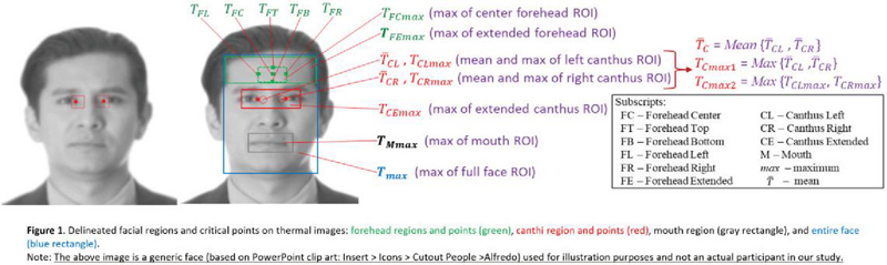
Figure 2 Region-Based Thermal Mapping of the Human Face: Forehead, Canthi, Mouth, and Full-Face ROIs (Region of Interest).

The class labels for the regression task are either the average oral temperature measured in fast mode (aveOralF) or the average temperature measured in monitor mode (aveOralM). Data were aquired and analyzed from a total of 1020 subject. In our research article we are using the 10% sample of the total population is 102 subject of the average temperature measured in monitor mode (aveOralM) by using the code $set.seed(123456)$ in R software. Now, We apply the Min-Max normalization technique, which scales the values of a feature to a range between 0 and 1. This is achieved by subtracting the feature’s minimum value from each data point and then dividing the result by the feature’s range. Two extreme observations, 0 and 1, were found and then removed from the dataset as a result of this method as given: 0.42 0.56 0.52 0.58 0.35 0.42 0.40 0.38 0.48 0.31 0.48 0.56 0.33 0.17 0.10 0.42 0.21 0.40 0.33 0.19 0.35 0.33 0.38 0.33 0.33 0.46 0.63 0.25 0.38 0.38 0.38 0.54 0.25 0.58 0.65 0.48 0.48 0.31 0.21 0.31 0.56 0.65 0.31 0.29 0.25 0.56 0.48 0.21 0.42 0.50 0.52 0.40 0.38 0.38 0.27 0.27 0.38 0.08 0.44 0.38 0.46 0.48 0.44 0.33 0.42 0.56 0.31 0.38 0.40 0.42 0.29 0.81 0.40 0.29 0.33 0.40 0.42 0.75 0.67 0.58 0.29 0.42 0.25 0.42 0.38 0.44 0.08 0.81 0.52 0.46 0.46 0.44 0.31 0.38 0.31 0.50 0.29 0.15 0.25 0.38.

From Tables 5, the skewness of the given dataset is approximately 0.3974, indicating a slight positive skew. The kurtosis is approximately 0.7143, suggesting that the dataset has a slightly higher peak and heavier tails compared to a normal distribution.

Table 5 The infrared thermography (IRT) temperature dataset

Data	Min.	1st quartile	Median	Mean	3rd quartile	Max.	Skewnss	Kurtosis
aveOralM	0.0800	0.3100	0.3900	0.4003	0.4800	0.8100	0.3974	0.7143

Table 6 Estimates, KS statistic and its p-values for the IRT temperature dataset

Model	Estimates	KS Test Statistic	P-value
Unit Omega Distribution	$\alpha =19.1933,\beta =3.5553$	0.0897	0.37472
Beta Distribution	$\alpha =6.0481,\beta =9.2360$	0.0952	0.30587

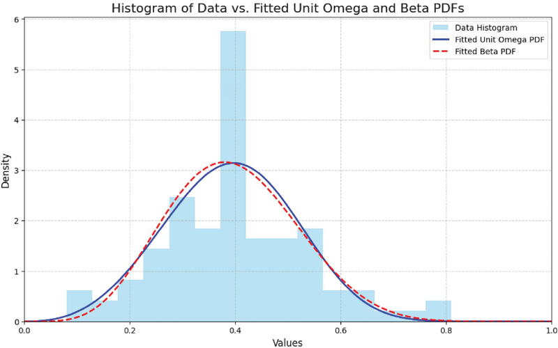
Figure 3 Empirical PDF vs. Fitted PDFs (Unit Omega vs Beta Distribution)

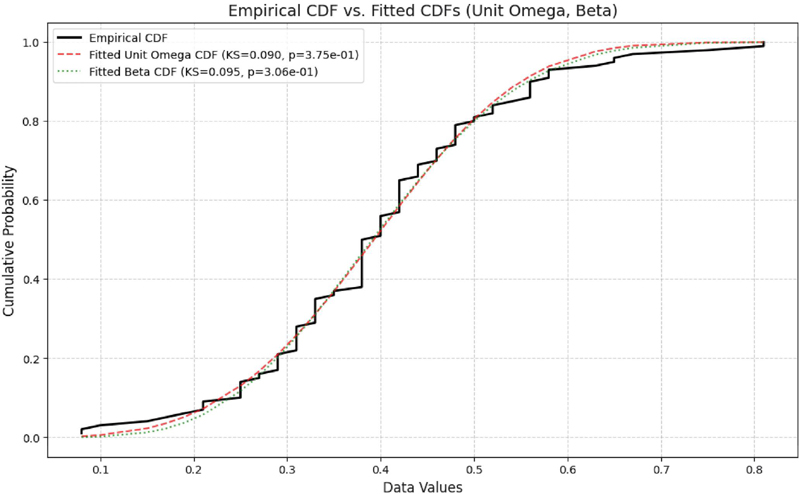
Figure 4 Empirical CDF vs. Fitted CDFs (Unit Omega vs Beta Distribution)

5.3 Assessment of Model Adequacy

The results of this study for the IRT Temperature Dataset are shown in Table 5 and 6 and the Power half normal shows overall better performance as compare to Normal Distribution and Exponential Distribution.

• Beta Distribution (Johnson et al. [27])

$$g(x;\alpha ,\beta )=\frac{1}{B(\alpha ,\beta )}{x}^{\alpha -1}{(1-x)}^{\beta -1};x\in (0,1),\alpha >0,\beta >0.$$

where

$$B(\alpha ,\beta )=\frac{\mathrm{\Gamma }(\alpha )\mathrm{\Gamma }(\beta )}{\mathrm{\Gamma }(\alpha +\beta )}$$

and $\mathrm{\Gamma }$ is the Gamma function.

Table 7 The k-th moments of the OSs of the the IRT temperature dataset

${\mu }_{r:20}^k$	$k=1$	$k=2$
r $=$ 1	0.757281	0.659466
r $=$ 2	0.727176	0.651588
r $=$ 3	0.702265	0.637143
r $=$ 4	0.682662	0.624020
r $=$ 5	0.666754	0.612664
r $=$ 6	0.653458	0.602809
r $=$ 7	0.642082	0.594163
r $=$ 8	0.632169	0.586490
r $=$ 9	0.623402	0.579610
r $=$ 10	0.615557	0.573384
r $=$ 11	0.608466	0.567705
r $=$ 12	0.602005	0.562491
r $=$ 13	0.596075	0.557674
r $=$ 14	0.590599	0.553201
r $=$ 15	0.585517	0.549029
r $=$ 16	0.580778	0.545121
r $=$ 17	0.576341	0.541448
r $=$ 18	0.572172	0.537984
r $=$ 19	0.568242	0.534708
r $=$ 20	0.564526	0.531601

5.4 The kth Moments of the OSs of the IRT Temperature Dataset

The kth moments of OSs: The smallest and largest observations among the order statistics (OSs) are particularly relevant for forecasting and estimating future events. Using Theorem 1, we do this by using the $k$th moments of chosen OSs that are obtained from the unit omega distribution. The matching L-moment estimates for the IRT Temperature data set are substituted for the involved parameters. Table 7 displays these OSs and shows that the moments decreases with an increase in $k$.

6 Concluding remarks

In this work, we examined the statistical characteristics of the Unit Omega distribution, focusing on its record values and moments of order statistics (OSs). The computation of single moments of order statistics was made easier by the establishment of helpful recursive linkages and the derivation of exact formulas for these variables. Additionally, utilizing the computed moments of order statistics and record values, a number of significant L-moment characteristics were found, offering further insight into the shape, variability, and tail behavior of the distribution. The suggested distribution was fitted to an original Infrared Thermography (IRT) temperature dataset to show its practical application, and its performance was contrasted with that of the Beta distribution, the most popular model for bounded data. The Unit Omega distribution provides a competitive and adaptable alternative for modeling bounded data, according to the empirical findings. A more thorough examination of order statistics and record values, the creation of inferential procedures under different censoring schemes, such as progressive censoring, and the investigation of reliability, survival, and lifetime analysis applications based on the Unit Omega distribution are just a few of the future research directions made possible by the findings presented in this work.

Conflicts of Interest

The authors declare no competing interests.

Authors’ Contributions

Mahfooz Alam and Alia A. Alkhathami proposed the concept of the paper and calculated the existing results. Mahfooz Alam, Showkat Ahmad Lone and Alia A. Alkhathami contributed in writing the original draft preparation and determined the existing results. Mahfooz Alam contributed to the methodology and concepts for the existing results. Aafaq A. Rather, Showkat Ahmad Lone and Mehdi Hosseinzadeh Alia A. Alkhathami revision and improved the quality of the draft. All authors have read and agreed to the published version of the Manuscrit.

Funding Statement

This research did not receive external funding.

Data Availability

https://doi.org/10.3390/s22010215.

Declaration of Generative AI and AI-assisted Technologies in the Writing Process

The authors only used Grammarly and QuillBot to improve their grammar and spelling. They are solely responsible for the content of the manuscript and all thoughts and analyses are their own.

Code Availability

We are using the R and Python software to calculate all the table values.

References

[1] Ahsanullah, M. (1995). Record Statistics. Nova Science Publishers, New York.

[2] Ahsanullah, M. and Nevzorov, V. B. (2015). Record via Probability Theory. Atlantis Press, Paris.

[3] Alam, M., Khan, R. U. and Athar, H. (2022). Lower record values from generalized inverse Weibull distribution. J. Math. Model., 10, 93–106.

[4] Alam, M., Khan, M. A. and Khan, R. U. (2020). Characterization of NH distribution through generalized record values. App. Math. E-Notes, 20, 406–414.

[5] Alam, M., Khan, M. A. and Khan, R. U. (2021). On upper $k$-record values from the generalized linear exponential distribution. J. Stat. Theory Appl., 20, 289–303.

[6] Alam, M., and Vidovic, Z. (2023). K-th Record Moments and Characterization of Inverted Nadarajag-Haghighi Distribution. Pakistan J. Statist. 39, 99–113.

[7] Alam, M., Barakat, H. M., Bakouch, H. S., and Chesneau, C. (2024). Order statistics and record values moments from the Topp-Leone Lomax distribution with applications to entropy. Wireless Personal Communications, 1–19.

[8] Almuhayfith, F. E., Alam, M., Bakouch, H. S., Bapat, S. R., and Albalawi, O. (2024). Linear Combination of Order Statistics Moments from Log-Extended Exponential Geometric Distribution with Applications to Entropy. Mathematics, 12(11), 1744.

[9] Arnold, B. C., Balakrishnan, N. and Nagaraja, H. N. (2008). A First Course in Order Statistics, SIAM Publishers, Philadelphia, USA.

[10] Alsubie, A., Akhter, Z., Athar, H., Alam, M., Ahmad, A. E. B. A., Cordeiro, G. M., & Afify, A. Z. (2021). On the omega distribution: Some properties and estimation. Mathematics, 9(6), 656.

[11] Arnold, B. C., Balakrishnan, N. and Nagaraja, H. N. (2011). Records. New York Wiley.

[12] Balakrishnan, N. and Cohen, A. C. (1992). Order statistics and inference estimation methods, J. R. Stat. Soc. A, 155, 307.

[13] Balakrishnan, N., Malik, H.J. and Ahmed, S.E. (1988): Recurrence relations and identities for moments of order statistics II: Specific continuous distributions, Comm. Statist. Theory Methods 17(8) 2657–2694.

[14] Balakrishnan, N. and Sultan, K.S. (1998): Recurrence relations and identities for moments of order statistics, In: N. Balakrishnan and C. R. Rao, eds., Handbook of Statistics, vol.16, 149-228, Order Statistics: Theory and Methods, North-Holland, Amsterdam, The Netherlands.

[15] Birbiçer, İ. and Genç, A. İ. (2022). On parameter estimation of the standard Omega distribution. Journal of Applied Statistics, 50(15), 3108–-3124. https://doi.org/10.1080/02664763.2022.2101045.

[16] Chandler, K. N. (1952): The distribution and frequency of record values, J. Roy. Statist. Soc. Ser. B, 14, 220–228.

[17] Çetinkaya, Ç., & Genç, A. İ. (2018). Moments of order statistics of the standard two-sided power distribution. Communications in Statistics-Theory and Methods, 47(17), 4311–4328.

[18] Comtet, L. (1974). Advanced Combinatiories. Boston: D. Riedel Publishing Company.

[19] David, H. A. and Nagaraja, H. N. (2003). Order Statistics. 3rd Edn. John Wiley, New York.

[20] Dombi, J., Jónás, T., Tóth, E.Z. and Árva, G. (2019): The Omega probability distribution and its applications in reliability theory. Qual. Reliab. Engng. Int., 35(2), 600–626.

[21] Dwight Chenna, Y. N., Ghassemi, P., Pfefer, T. J., Casamento, J., and Wang, Q. (2018). Free-form deformation approach for registration of visible and infrared facial images in fever screening. Sensors, 18(1), 125. https://doi.org/10.3390/s18010125.

[22] Ghassemi, P., Pfefer, T. J., Casamento, J. P., Simpson, R., and Wang, Q. (2018). Best practices for standardized performance testing of infrared thermographs intended for fever screening. PLOS ONE, 13(9), e0203302. https://doi.org/10.1371/journal.pone.0203302.

[23] Ghitany, M. E., Mazucheli, J., Menezes, A. F. B., and Alqallaf, F. (2019). The unit-inverse Gaussian distribution: A new alternative to two-parameter distributions on the unit interval. Communications in Statistics-Theory and methods, 48(14), 3423–3438.

[24] Gradshteyn, I.S. and Ryzhik, I.M. (2007): Tables of Integrals, Series and Products. Edited by Jeffrey, A. and Zwillinger, D. 7th Ed., Academic Press, San Diego.

[25] Hosking, J. R. M., and Wallis, J. R. (1997). Regional frequency analysis (p. 240).

[26] Hosking, J. R. M. (1990). L-moments: analysis and estimation of distributions using linear combinations of order statistics. J. Roy. Statist. Soc. B, 52(1), 105–124.

[27] Johnson, N. L., Kotz, S., and Balakrishnan, N. (1995). Continuous univariate distributions, volume 2. John wiley & sons.

[28] Jónás, T., and Bakouch, H. S. (2022). The generalized omega function and its connection with some probability distributions. Mediterranean Journal of Mathematics, 19(6), 250.

[29] Khan, A.H., Yaqub, M. and Parvez, S. (1983a): Recurrence relations between moments of order statistics. Naval Research Logistics Quarterly, 30, 419-441. [Corrections, 32, (1985) 693]

[30] Korkmaz, M. Ç. (2020). The unit generalized half normal distribution: A new bounded distribution with inference and application.

[31] Malik, H.J., Balakrishnan, N. and Ahmed, S.E. (1988): Recurrence relations and identities for moments of order statistics I: Arbitrary continuous distribution, Comm. Statist. Theory Methods 17(8) 2632–2655.

[32] Martinez-Florez, G., Olmos, N. M., and Venegas, O. (2024). Unit-bimodal Birnbaum-Saunders distribution with applications. Communications in Statistics-Simulation and Computation, 53(5), 2173– 2192.

[33] Mathai, A. M. and Saxena, R. K. (1973). Generalized hyper-geometric functions with applications in statistics and physical science. Lecture Notes in Mathematics. 348, Springer-Veriag, Berlin.

[34] Maya, R., Jodra, P., Irshad, M. R., and Krishna, A. (2024). The unit Muth distribution: Statistical properties and applications. Ricerche di Matematica, 73(4), 1843–1866.

[35] Mazucheli, J., A. F. B. Menezes, and M. E. Ghitany. “The unit-Weibull distribution and associated inference.” J. Appl. Probab. Stat 13.2 (2018): 1–22.

[36] Mazucheli, J., Menezes, A. F. B., and Chakraborty, S. (2019). On the one parameter unit-Lindley distribution and its associated regression model for proportion data. Journal of Applied Statistics, 46(4), 700–714.

[37] Nadarajah, S. (2008). Explicit expressions for moments of order statistics. Statistics & Probability Letters, 78(2), 196–205.

[38] Nagaraja, H. N. (2013). Moments of order statistics and L-moments for the symmetric triangular distribution. Statistics & Probability Letters, 83(10), 2357–2363.

[39] Okorie, I. E., and Nadarajah, S. (2019). On the omega probability distribution. Quality and Reliability Engineering International, 35(6), 2045–2050.

[40] Özbilen, Ö., and Genç, A. İ. (2022). A bivariate extension of the Omega distribution for two-dimensional proportional data. Mathematica Slovaca, 72(6).

[41] Prataviera, F. and Cordeiro, G. M. (2024). The Unit Omega Distribution, Properties and Its Application. American Journal of Mathematical and Management Sciences, 1–-14. https://doi.org/10.1080/01966324.2024.2310648.

[42] Ribeiro-Reis, L. D. (2021). Unit log-logistic distribution and unit log-logistic regression model. Journal of the Indian Society for Probability and Statistics, 22(2), 375–388.

[43] Singh, B., Alam, I., Rather, A. A., and Alam, M. (2023). Linear combination of order statistics of exponentiated Nadarajah–Haghighi distribution and their applications. Lobachevskii Journal of Mathematics, 44(11), 4839–4848.

[44] Wang, Q., Zhou, Y., Ghassemi, P., McBride, D., Casamento, J. and Pfefer, T., (2022): Infrared Thermography for Measuring Elevated Body Temperature: Clinical Accuracy, Calibration, and Evaluation. Sensors, 22, 215. https://doi.org/10.3390/s22010215.

[45] Yousaf, F., Ali, S., and Shah, I. (2019). Statistical inference for the Chen distribution based on upper record values. Annals of Data Science, 6(4), 831–851.

[46] Yousaf, F., Ali, S., Shah, I., and Riaz, S. (2023). Parameters estimation of the exponentiated chen distribution based on upper record values. Journal of Reliability and Statistical Studies, 197–228.

[47] Zhou, Y., Ghassemi, P., Chen, M., McBride, D., Casamento, J. P., Pfefer, T. J., and Wang, Q. (2020). Clinical evaluation of fever-screening thermography: Impact of consensus guidelines and facial measurement location. Journal of Biomedical Optics, 25(9), 097002. https://doi.org/10.1117/1.JBO.25.9.097002.

Biographies

Alia A. Alkhathami is an Assistant Professor of Mathematics and Statistics at Saudi Electronic University (SEU), Kingdom of Saudi Arabia. She earned her M.Sc. in Probability and Statistics, from Carleton University, Canada, in 2015 and her Ph.D. in Probability and Statistics, from Carleton University, Canada, in 2021. Her research interests include Statistics, missing data analysis, longitudinal data analysis and applied statistical modeling, and she has published extensively in reputed international journals. She actively contributes to research in reliability analysis and statistical methodologies.

Mahfooz Alam recently joined Vishwakarma University as assistant professor in the department of Mathematics and Statistics. He is currently working on moment properties in ordered random variates such as order statistics, record values, progressive censoring, generalized order statistics, dual generalized order statistics and the characterizations of continuous probability distributions. He has published several research papers in the reputated journal of national and international.

Aafaq A. Rather is an Assistant Professor at the Symbiosis Statistical Institute, India. He has published more than 130 research papers in SCI, ESCI, Scopus-indexed, and other reputed international journals. His research interests include probability distributions, reliability analysis, survival analysis and statistical modeling. Dr. Rather is actively involved in research supervision and has contributed significantly to the field of applied statistics through his academic and research activities.

Mehdi Hosseinzadeh is the Director of the DTU AI & Data Science Hub (DAIDASH) at Duy Tan University. He has authored over 500 peer-reviewed publications and supervised more than 120 postgraduate researchers, with an h-index above 95. His research focuses on artificial intelligence, deep learning, health informatics, recommender systems, IoT, and data analytics. He has been recognized among the world’s top 2% scientists from 2022 to 2025.

Showkat Ahmad Lone is an Associate Professor of Mathematics and Statistics at Saudi Electronic University (SEU), Kingdom of Saudi Arabia. He earned his M.Sc. in Statistics from the University of Kashmir in 2013 and his Ph.D. in Statistics, specializing in Reliability Engineering, from Aligarh Muslim University, India, in 2017. His research interests include Statistics, Reliability Engineering, and applied statistical modeling, and he has published extensively in reputed international journals. He actively contributes to research in reliability analysis and statistical methodologies and serves as a reviewer for several leading scientific journals. In recognition of his outstanding research impact and scholarly contributions, he was recently included in Stanford University’s Top 2% Scientists list.

Journal of Reliability and Statistical Studies, Vol. 19, Issue 2 (2026), 473–498
doi: 10.13052/jrss0974-8024.19210
© 2026 River Publishers