Statistical Inference for Gompertz and Weibull Models under Doubly Interval-Censored Data

Himani Kotian¹, Sunita Sharma^2,*, Asha Kamath³ and Vasudeva Guddattu⁴

¹Department of Community Medicine, Kasturba Medical College Mangalore, Manipal Academy of Higher Education, Manipal, India
²Manipal Institute of Technology, Manipal Academy of Higher Education, Manipal, India
³Department of Applied Statistics & Data Science, Prasanna School of Public Health, Manipal Academy of Higher Education, Manipal, India
⁴Department of Applied Statistics & Data Science, Prasanna School of Public Health, Manipal Academy of Higher Education, Manipal, India
E-mail: sunita.sharma@manipal.edu
*Corresponding Author

Received 28 March 2026; Accepted 10 August 2026

ABSTRACT

This study explores the statistical inference for the Gompertz model using doubly interval-censored data. In this framework, the initial event time is assumed to follow either a Weibull or uniform distribution, whereas the lifetime of interest is assumed to follow the Gompertz distribution. Confidence intervals for the model parameters were constructed using the Wald and likelihood ratio methods and compared in terms of coverage probability. A simulation study was conducted to examine the large-sample asymptotic behavior of the estimators and the interval procedures. The results indicate that the Wald method consistently provides more accurate and reliable coverage than the likelihood ratio method. A real-life dataset was analyzed to validate the proposed methodology and to demonstrate its practical relevance.

Keywords: Doubly interval censoring, likelihood ratio, Wald method, Gompertz model, coverage probability.

Introduction

Doubly interval-censored data (DICD) extends the concept of censoring by considering survival time as the duration between two interconnected events: the initial event ($U$) and the subsequent event ($V$), both of which may be subject to interval censoring (IC). In contrast, interval censoring specifies that the event’s timing falls within a defined interval. DICD is often encountered in epidemiological or disease progression studies, where the first and second events could represent the onset of an infection and the development of a disease, respectively. In HIV-AIDS studies, $U$ denotes the time of HIV infection, which is not directly observed but is known to lie within an interval $(U_L,U_R)$, where $U_L$ is the time of the last negative antibody test and $U_R$ is the time of the first positive antibody test. The variable $V$ represents the time of AIDS diagnosis. This time may be exactly observed ($V_L=V_R$) or right censored ($V_R=+\mathrm{\infty }$) for individuals who have not developed AIDS by the end of the study period. The elapsed time between infection and AIDS diagnosis, defined as $T=V-U$, is referred to as the AIDS latency (or incubation) time (Calle 2002). Since the HIV infection time is only known to occur between the last negative test and the first positive test, it is frequently measured by routine blood testing. As a result, observations are frequently interval censored. Additionally, because of factors including the study’s conclusion and its monthly follow-up design, observations regarding AIDS diagnoses may be either right censored (RC) or IC, producing DICD on T (De Gruttola and Lagakos, 1989; Kim, et al., 1993; Calle 2002; Loh et al., 2017). For example, the value of $U$ is interval-censored if the exact value is unknown with $U\in (U_L,U_R]$, and $V$ is similarly defined as interval-censored with $V\in (V_L,V_R]$. Consequently, the survival time ($T$) is considered doubly interval-censored when its exact value is unknown but is known to lie within the interval ($V_L-U_R,V_R-U_L$ ] satisfying the condition $V_L-U_R\le V_R-U_L$, ensuring that the intervals for events $V$ and $U$ are consistent with the observed data (Loh et al. 2017; Yin et al., 2021).

Let the probability density functions of $U,T$, and $V$ be $f_u(u),f_T(t)$ and $f_v(v)$ respectively. For given $v$ and $t=v-u$, the joint probability density function (PDF) of $U$ and $V,f(u,v)=$ $f_u(u)f_T(v-u)$, with the likelihood function given below:

$$L(\lambda ,\gamma )={\int }_{v_L}^{v_R}{\int }_{u_L}^{u_R}{f}_u(u)f_T(v-u)\mathit{d}v\mathit{d}u$$

(1)

where $\lambda$ represents the parameter associated with the probability density functions $f_u$ and $f_T$ (Loh et al., 2017; Calle 2002).

Kiani and Arasan (2012) proposed a parametric model for the analysis of doubly interval-censored data (DICD) under the assumption that both the initial event time, (U), and the lifetime of interest, (T), follow exponential distributions. Subsequently, Kiani and Arasan (2017) extended this line of research by proposing a parametric model in which the initial event time (U) follows a Uniform distribution and the survival time (T) follows a special case of the log-logistic distribution. Motivated by these studies, the present research proposes a new parametric model for the analysis of DICD. Specifically, the initial event time (U) is assumed to follow either a Weibull or a Uniform distribution, while the lifetime of interest (T) is assumed to follow a Gompertz distribution. A simulation study was conducted to investigate the large-sample asymptotic properties of the proposed estimators and the associated interval estimation procedures. Furthermore, unlike the previous studies, which focused primarily on methodological development and simulation-based evaluations, the present study incorporates the analysis of a real-life dataset to validate the proposed methodology and demonstrate its practical applicability. The mathematical novelty of this study lies in exploring the combination of the Weibull and Gompertz distributions for modeling DICD.

Case 1

Let $T$ be the lifetime of interest. If U is the initial event time and V is the subsequent event time, then $T=V-U$.

The Likelihood for a doubly interval censored lifetime is

$${\int }_{v_L}^{v_R}{\int }_{u_L}^{u_R}{f}_u(u)f_T(v-u)\mathit{d}v\mathit{d}u$$

(2)

Where

$U\in (U_L,U_R)$ with $U_L\le U_R$

$V\in (V_L,V_R)$ with $V_L\le V_R$

In Equation (1), $f_u(u)$ and $f_T(t)$ are the density functions of $U$ and, $T$ respectively. Assumed that the initial time event $U$ follows a Weibull distribution and the lifetime of interest T follows a Gompertz distribution.

The Model

We assume that initial event $U\sim W(\alpha ,\lambda )$, $\alpha$ as shape parameter; $\lambda$ as scale parameter.

With PDF

$$f_u(u)=\alpha \lambda {(\lambda u)}^{\alpha -1}{e}^{-{(u\lambda )}^{\alpha }};u\ge 0$$

(3)

and cumulative distribution function (CDF) is given by

$$F(u)=1-e^{-{(u\lambda )}^{\alpha }};u\ge 0$$

(4)

The Survival function is defined as

$S(u)$	$=1-F(u)$
	$=1-(1-e^{-{(u\lambda )}^{\alpha }})$
$S(u)$	$=e^{-{(u\lambda )}^{\alpha }};u\ge 0$	(5)

and the Hazard failure rate (HFR) function is

$h(u)$	$={\displaystyle \frac{f(u)}{\mathrm{s}(\mathrm{u})}}={\displaystyle \frac{\alpha \lambda {(\lambda u)}^{\alpha -1}{e}^{-{(\lambda u)}^{\alpha }}}{e^{-{(u\lambda )}^{\alpha }}}}$
$h(u)$	$=\alpha \lambda {(\lambda u)}^{\alpha -1};u\ge 0$	(6)

The lifetime $T$ follows Gompertz distribution with PDF

$$f(t)=\gamma \exp (\beta t)\times \exp \left[\frac{\gamma }{\beta }\left(1-e^{\beta t}\right)\right]t\ge 0,\gamma >0,\beta >0$$

(7)

The Survival and Hazard function of the Gompertz model are given by

$S(t)=\exp \left[{\displaystyle \frac{\gamma }{\beta }}(1-e^{\beta t})\right]$

(8)

and

$h(t)=\gamma \exp (\beta t);t\ge 0,\gamma >0,\beta >0$

(9)

$T$ is the survival time of interest.

$f_t(T)$ is the density function.

where $f_u(U)$ and $f_v(V)$ denote the density function of the time to occurrence of the first event $U$ and second event V respectively. According to Reich et al. (2009), the distribution of $V$ can be obtained if $U$ is given and $f_t(T)$ is known. Thus, we have

$$f_{v|u}(v|u)=f_t(v-u|u)$$

(10)

Then, the joint density function of $V$ and $U$ would be

$f_{u,v}(u,v)$	$=f_{v|u}(v|u)f_u(U)$
	$=f_t(v-u|u)\times f_u(U)$
$f_{u,v}(u,v)$	$=f_t(v-u)\times f_u(U)$	(11)

where $T=V-U$ and U are assumed to be independent of $T$ (Oller, et al., 2004). The independence between $U$ and $T$, which are classical assumptions for the treatment of DICD survival times, Therefore, the likelihood for doubly interval- censored data is

$$L={\int }_{U_L}^{U_R}{\int }_{V_L}^{V_R}{f}_{U,V}(U,V)\mathit{d}u\mathit{d}v$$

$${\int }_{v_L}^{v_R}{\int }_{u_L}^{u_R}{f}_u(u)f_T(v-u)\mathit{d}v\mathit{d}u$$

This is similar to Equation (1).

Where $U\sim W(\alpha ,\lambda )$ and $T\sim \mathrm{Gompertz}(\gamma ,\beta )$.

When both $U$ and $V$ are IC and T is DIC, the likelihood function is derived as

$L$	$={\displaystyle {\int }_{U_L}^{U_R}}{\displaystyle {\int }_{V_L}^{V_R}}\gamma \exp (\beta (v-u))$
	$\times \exp \left[{\displaystyle \frac{\gamma }{\beta }}\left(1-e^{\beta (v-u)}\right)\right]\alpha \lambda {(\lambda u)}^{\alpha -1}{e}^{-{(\lambda u)}^{\alpha }}dvdu$	(12)
	$=\gamma \alpha \lambda {(u)}^{\alpha -1}{\displaystyle {\int }_{U_L}^{U_R}}{\displaystyle {\int }_{V_L}^{V_R}}\exp (\beta (v-u))$
	$\times \exp \left[{\displaystyle \frac{\gamma }{\beta }}\left(1-e^{\beta (v-u)}\right)\right]u^{\alpha -1}{e}^{-{(\lambda u)}^{\alpha }}dvdu$
	$=\gamma \alpha {\lambda }^{\alpha }{\displaystyle {\int }_{U_L}^{U_R}}{\displaystyle {\int }_{V_L}^{V_R}}{e}^{(\beta (v-u))}{e}^{\frac{\gamma }{\beta }\left(1-e^{\beta (v-u)}\right)}\cdot u^{\alpha -1}{e}^{-{(\lambda u)}^{\alpha }}\mathit{d}v\mathit{d}u$
	$=\gamma \alpha {\lambda }^{\alpha }{\displaystyle {\int }_{U_L}^{U_R}}{\displaystyle {\int }_{V_L}^{V_R}}{e}^{(\beta (v-u))+\frac{\gamma }{\beta }\left(1-e^{\beta (v-u)}\right)}{u}^{\alpha -1}{e}^{-{(\lambda u)}^{\alpha }}\mathit{d}v\mathit{d}u$
	$=\gamma \alpha {\lambda }^{\alpha }{\displaystyle {\int }_{U_L}^{U_R}}{u}^{\alpha -1}{e}^{-{(\lambda u)}^{\alpha }}\left[{\displaystyle {\int }_{V_L}^{V_R}}{e}^{(\beta (v-u))}{e}^{\frac{\gamma }{\beta }\left(1-e^{\beta (v-u)}\right)}\right]\mathit{d}v\mathit{d}u$
$L$	$=\gamma \alpha {\lambda }^{\alpha }{\displaystyle {\int }_{U_L}^{U_R}}{u}^{\alpha -1}{e}^{-{(\lambda u)}^{\alpha }}$
	$\times [{\displaystyle {\int }_{V_L}^{V_R}}\exp (\beta (v-u))+{\displaystyle \frac{\gamma }{\beta }}(1-e^{\beta (v-u)})]dvdu]$	(13)

Substitute inner integral in the above equation.

Let

$z$	$=v-u$
$v$	$=z+u$
$dv$	$=dz$

And the limits of the integral become when $z=V_L-u$ for lower limit and $z=V_R-u$ for upper limit

So, the inner integral becomes,

$$L={\int }_{V_L-u}^{V_R-u}\exp \left(\beta z+\frac{\gamma }{\beta }(1-e^{\beta z})\right)\mathit{d}z$$

(14)

So, the final integral expression is formulated as

$L$	$=\gamma \alpha {\lambda }^{\alpha }{\displaystyle {\int }_{U_L}^{U_R}}{u}^{\alpha -1}{e}^{-{(\lambda u)}^{\alpha }}$
	$\times \left[{\displaystyle {\int }_{V_L-u}^{V_R-u}}\left(\exp \left(\beta z+{\displaystyle \frac{\gamma }{\beta }}\left(1-e^{\beta z}\right)\right)dz\right)\mathit{d}u\right]$	(15)

The inner integral over $z$ cannot be evaluated analytically for general values of $\beta$ and $\gamma$. Therefore, we can use numerical techniques to obtain the solution.

The censoring indicators for the $i$th subject are defined as follows, according to the reference article (Loh et al. 2017)

${\delta }_{D{C}_i}=1$ if $T$ is DIC; 0 otherwise.

${\delta }_{I{R}_i}=1$ if $U$ is IC and $V$ is RC; 0 otherwise.

${\delta }_{I{C}_i}=1$ if $T$ is IC and 0 otherwise.

${\delta }_{R{C}_i}=1$ if $T$ is RC and 0 otherwise.

${\delta }_{O{E}_i}=1$ if $T$ is OE; 0 otherwise.

where ${\delta }_{O{E}_i}=1-\left({\delta }_{D{C}_i}+{\delta }_{I{R}_i}+{\delta }_{I{C}_i}+{\delta }_{R{C}_i}\right)$ Subsequently, the likelihood function is for the full sample can be written as

$L(\gamma ,\beta )$	$={\displaystyle \prod _{i=1}^n}[\gamma \alpha {\lambda }^{\alpha }{\displaystyle {\int }_{U_L}^{U_R}}{u}^{\alpha -1}{e}^{-{(\lambda u)}^{\alpha }}$
	$\times {\left[{\displaystyle {\int }_{V_L-u}^{V_R-u}}\left(\exp \left(\beta z+{\displaystyle \frac{\gamma }{\beta }}\left(1-e^{\beta z}\right)\right)dz\right)\mathit{d}u\right]}^{{\delta }_{D{C}_i}}$
	$\times {\displaystyle \prod _{i=1}^n}\gamma \alpha {\lambda }^{\alpha }{\displaystyle {\int }_{U_{L_i}}^{U_{R_i}}}{u}^{\alpha -1}{e}^{-{(\lambda u)}^{\alpha }}$
	$\times {\left[{\displaystyle {\int }_{V_{L_i}-u}^{\mathrm{\infty }}}\left(\exp \left(\beta z+{\displaystyle \frac{\gamma }{\beta }}\left(1-e^{\beta z}\right)\right)dz\right)\mathit{d}u\right]}^{{\delta }_{I{R}_i}}$
	$\times {\left[\exp {\displaystyle \frac{\gamma }{\beta }}(1-e^{\beta (t_{L_i}-t_{R_i})})\right]}^{{\delta }_{I{C}_i}}$
	$\times [\exp {\left[{\displaystyle \frac{\gamma }{\beta }}(1-e^{-\beta t_{o_i}})\right]}^{{\delta }_{R{C}_i}}$
	$\times {[\gamma \exp (\beta t_i)\times \exp {\displaystyle \frac{\gamma }{\beta }}(1-e^{\beta t_i})]}^{{\delta }_{O{E}_i}}]$	(16)

After taking log of the likelihood function

$\log L(\gamma ,\beta )$	$={\displaystyle \sum _{i=1}^n}\{{\delta }_{D{C}_i}\log ((\gamma \alpha {\lambda }^{\alpha }{\displaystyle {\int }_{U_L}^{U_R}}{u}^{\alpha -1}{e}^{-{(\lambda u)}^{\alpha }}$
	$\times [{\displaystyle {\int }_{V_L-u}^{V_R-u}}\left(\exp (\beta z+{\displaystyle \frac{\gamma }{\beta }}(1-e^{\beta z})dz)du\right)$
	$+{\delta }_{I{R}_i}\log (\gamma \alpha {\lambda }^{\alpha }{\displaystyle {\int }_{U_{L_i}}^{U_{R_i}}}{u}^{\alpha -1}{e}^{-{(\lambda u)}^{\alpha }}$
	$\times \left[{\displaystyle {\int }_{V_{L_i}-u}^{\mathrm{\infty }}}\left(\exp \left(\beta Z+{\displaystyle \frac{\gamma }{\beta }}(1-e^{\beta Z})\right)\right)\mathit{d}z\mathit{d}u\right]$
	$+{\delta }_{I{C}_i}\left[{\displaystyle \frac{\gamma }{\beta }}+\beta (t_{L_i}-t_{R_i})\right]+{\delta }_{R{C}_i}\left[{\displaystyle \frac{\gamma }{\beta }}(1-e^{-\beta t_{o_i}})\right]$
	$+{\delta }_{O{E}_i}[\log \gamma +\beta t_i+{\displaystyle \frac{\gamma }{\beta }}+\log (1-e^{\beta t_i})]\}$	(17)

The maximum likelihood estimator (MLE) of the parameters is obtained using the Newton-Raphson algorithm.

Case 2

Let $T$ be the lifetime of interest, if $U$ is the initial event time, $V$ is the subsequent event time and $T=V-U$.

The Likelihood for a doubly interval censored lifetime is

$${\int }_{v_L}^{v_R}{\int }_{u_L}^{u_R}{f}_u(u)f_T(v-u)\mathit{d}v\mathit{d}u$$

Where

$U\in (U_L,U_R)$ with $U_L\le U_R$

$V\in (V_L,V_R)$ with $V_L\le V_R$

In Equation (1), $f_u(u)$ and $f_T(t)$ are the density functions of $U$ and, $T$ respectively. Assumed that the initial time event $U$ follows Uniform distribution and the lifetime of interest follows Gompertz distribution.

$U$	$=U(U_L,U_R),T\sim \text{gompertz}(\gamma ,\beta );\gamma >0,\beta >0$
$L$	$={\displaystyle {\int }_{U_L}^{U_R}}{\displaystyle {\int }_{V_L}^{V_R}}{f}_{U,V}(U,V)\mathit{d}u\mathit{d}v$
	$={\displaystyle {\int }_{v_L}^{v_R}}{\displaystyle {\int }_{u_L}^{u_R}}{f}_u(u)f_T(v-u)\mathit{d}v\mathit{d}u$

Here $U\sim U(U_L,U_R)$ and $T\sim \mathrm{Gompertz}(\gamma ,\beta )$.

When both $U$ and $V$ are IC, T is DICD, and the likelihood contribution is

$L$	$={\displaystyle {\int }_{U_L}^{U_R}}{\displaystyle {\int }_{V_L}^{V_R}}\gamma e^{(\beta (v-u)}\exp \left[{\displaystyle \frac{-\gamma }{\beta }}\left(e^{\beta (v-u)}-1\right)\right]$
	$\ast {\displaystyle \frac{1}{\left(U_R-U_L\right)}}dvdu$
$L$	$={\displaystyle \frac{1}{(U_R-U_L)}}{\displaystyle {\int }_{U_L}^{U_R}}{\displaystyle {\int }_{V_L}^{V_R}}\gamma e^{(\beta (v-u)}\exp \left[{\displaystyle \frac{-\gamma }{\beta }}(e^{\beta (v-u)}-1)\right]\mathit{d}v\mathit{d}u$	(18)

Therefore, the inner integral equals,

${\displaystyle {\int }_{V_L}^{V_R}}{f}_T(V-U)\mathit{d}u$	$={\displaystyle {\int }_{t_1=V_{L-U}}^{t_2=V_R-U}}{f}_T(t)\mathit{d}t$
	$=\left[S_t\left(t_1\right)-S_t\left(t_2\right)\right]$
	$=\exp \left[{\displaystyle \frac{-\gamma }{\beta }}(e^{\beta t_1}-1)\right]-\exp \left[{\displaystyle \frac{-\gamma }{\beta }}(e^{\beta t_2}-1)\right]$

We know that for Gompertz distribution,

$S_t(t)$	$=\exp \left[{\displaystyle \frac{-\gamma }{\beta }}(1-e^{\beta t})\right];t\ge 0$	(19)
$L$	$={\displaystyle \frac{1}{(U_R-U_L)}}{\displaystyle {\int }_{U_L}^{U_R}}\exp \left[{\displaystyle \frac{-\gamma }{\beta }}(e^{\beta (V_L-u)}-1)\right]$
	$-\exp \left[{\displaystyle \frac{-\gamma }{\beta }}(e^{\beta (V_R-u)}-1)\right]du$
$L$	$={\displaystyle \frac{1}{\left(U_R-U_L\right)}}{\displaystyle {\int }_{U_L}^{U_R}}{e}^{\frac{-\gamma }{\beta }\left(e^{\beta \left(V_L-U\right)}-1\right)}-e^{\frac{-\gamma }{\beta }\left(e^{\beta \left(V_R-U\right)}-1\right)}du$	(20)

Let $\frac{\gamma }{\beta }=k$.

So $L$ becomes

$$L=\frac{1}{(U_R-U_L)}{\int }_{U_L}^{U_R}{e}^{-k(e^{\beta (V_L-U)}-1)}-e^{-k(e^{\beta \left(V_R-U\right)}-1)}du$$

(21)

In general, we consider, $e^{-k(e^{\beta (V-U)}-1)}$. Hence, integral of $e^{-k(e^{\beta (V-U)}-1)}$ is

${\displaystyle {\int }_{U_L}^{U_R}}{e}^{-k\left(e^{\beta (V-U)}-1\right)}\mathit{d}u$	$={\displaystyle {\int }_{U_L}^{U_R}}{\displaystyle \frac{1}{e^{k\left(e^{\beta (V-U)}-1\right)}}}\mathit{d}u$
	$={\displaystyle {\int }_{U_L}^{U_R}}{\displaystyle \frac{1}{e^{kz}}}\ast {\displaystyle \frac{-\beta }{(1+Z)}}\mathit{d}z$
	$={\displaystyle {\int }_{U_L}^{U_R}}{\displaystyle \frac{-\beta }{(1+Z)}}{e}^{-KZ}\mathit{d}z$
	$=-\beta {\displaystyle {\int }_{U_L}^{U_R}}{\displaystyle \frac{e^{-KZ}}{(1+Z)}}\mathit{d}z$	(22)

Using this transformation.

Let

$e^{\beta (V-U)}-1$	$=z=e^{\beta (V-U)}=1+z$
${\displaystyle \frac{e^{\beta (V-U)}}{-\beta }}du$	$=dz$
$e^{\beta (V-U)}du$	$=-\beta dz$
$(1+z)du$	$=-\beta dz$

Now, applying new limits, after the transformation of variables, we obtain the limits of $Z$ as

$e^{\beta \left(V-U_L\right)}-1=z_1$ where $U=U_L$

$e^{\beta \left(V-U_R\right)}-1=z_2$ where $U=U_R$

So,

$L$	$=-\beta {\displaystyle {\int }_{e^{\beta {(V-U_L)}_{-1}}}^{e^{\beta {(V-U_R)}_{-1}}}}{\displaystyle \frac{e^{-KZ}}{(1+z)}}\mathit{d}z$
$L$	$={\displaystyle \frac{-\beta }{(U_R-U_L)}}{\displaystyle {\int }_{e^{\beta {(V-U_L)}_{-1}}}^{e^{\beta (V-U_R)}-1}}{\displaystyle \frac{e^{-Kz}}{(1+z)}}\mathit{d}z$	(23)

Take $1+z=y,dy=dz$ and the integration limits changes to,

$y_1=1+z_1=e^{\beta (V-U_L)}$

$y_2=1+z_2=e^{\beta (V-U_R)}$

and $\frac{e^{-Kz}}{(1+z)}=\frac{e^{-K(y-1)}}{y}=\frac{e^k{e}^{-ky}}{y}$.

Can be now written as below equation,

$$L=\frac{-\beta e^k}{(U_R-U_L)}{\int }_{e^{\beta {(V-U_L)}_{-1}}}^{e^{\beta {(V-U_R)}_{-1}}}\frac{e^{-Ky}}{y}\mathit{d}y$$

(24)

The antiderivative of $\frac{e^{-Ky}}{y}$ is the exponential integral $Ei(-ky)$ [Since $\frac{d}{dy}Ei(-ky)=\frac{e^{-Ky}}{y}$].

Therefore,

$L$	$={\displaystyle \frac{-\beta e^k}{(U_R-U_L)}}[Ei(-k{y}_2)-Ei(-k{y}_1)]$
$L$	$={\displaystyle \frac{-\beta e^k}{(U_R-U_L)}}[Ei(-k{e}^{\beta (V-U_R)})-Ei(-k{e}^{\beta (V-U_L)})]$	(25)

This $Ei(x)={\int }_{-\mathrm{\infty }}^x\frac{e^t}{t}\mathit{d}t$ is called special function.

The censoring indicators for the $i$th subject are defined as follows, according to the reference article (Loh et al., 2017)

${\delta }_{D{C}_i}=1$ if $T$ is DIC;0 otherwise.

${\delta }_{I{R}_i}=1$ if $U$ is IC and $V$ is RC; 0 otherwise.

${\delta }_{I{C}_i}=1$ if $T$ is IC and 0 otherwise.

${\delta }_{R{C}_i}=1$ if $T$ is RC and 0 otherwise.

${\delta }_{O{E}_i}=1$ if $T$ is OE;0 otherwise.

Where, ${\delta }_{{\mathrm{OE}}_{\mathrm{i}}}=1-\left({\delta }_{{\mathrm{DC}}_{\mathrm{i}}}+{\delta }_{{\mathrm{IR}}_{\mathrm{i}}}+{\delta }_{{\mathrm{IC}}_{\mathrm{i}}}+{\delta }_{{\mathrm{RC}}_{\mathrm{i}}}\right)$. Subsequently, the likelihood function for the full sample can be written as

$L((\gamma ,\beta )$	$={\displaystyle \prod _{i=1}^n}{\displaystyle \frac{-\beta e^k}{(U_R-U_L)}}{[Ei(-k{e}^{\beta (V-U_R)})Ei(-k{e}^{\beta (V-U_L)})]}^{{\delta }_{{\mathrm{DC}}_{\mathrm{i}}}}$
	$\times {\displaystyle \prod _{i=1}^n}{\displaystyle \frac{-\beta e^k}{(U_R-U_L)}}{[Ei(-k{e}^{\beta (V-U_R)})-Ei(-k{e}^{\beta (V-U_L)})]}^{{\delta }_{{\mathrm{IR}}_{\mathrm{i}}}}$
	$\times {\left[\exp {\displaystyle \frac{\gamma }{\beta }}(1-e^{\beta (t_{L_i}-t_{R_i})})\right]}^{{\delta }_{I{C}_i}}\times {\left[\exp {\displaystyle \frac{\gamma }{\beta }}(1-e^{-\beta t_{o_i}})\right]}^{{\delta }_{R{C}_i}}$
	$\times {\left[\gamma \exp (\beta t_i)\times \exp {\displaystyle \frac{\gamma }{\beta }}(1-e^{\beta t_i})\right]}^{{\delta }_{O{E}_i}}$	(26)

After taking log of the likelihood function

$\log L(\gamma ,\beta )$	$={\displaystyle \sum _{i=1}^n}\{{\delta }_{D{C}_i}\log ({\displaystyle \frac{-\beta e^k}{(U_R-U_L)}}[Ei(-k{e}^{\beta (V-U_R)})$
	$-Ei(-k{e}^{\beta (V-U_L)})]$
	$+{\delta }_{I{R}_i}\log ({\displaystyle \frac{-\beta e^k}{(U_R-U_L)}}[Ei(-k{e}^{\beta (V-U_R)})$
	$-Ei(-k{e}^{\beta (V-U_L)})]+\delta {}_{I{C}_i}[{\displaystyle \frac{\gamma }{\beta }}+\beta (t_{L_i}-t_{R_i})]$
	$+{\delta }_{R{C}_i}\left[{\displaystyle \frac{\gamma }{\beta }}(1-e^{-\beta t_{o_i}})\right]$
	$+{\delta }_{O{E}_i}[\log \gamma +\beta t_i+{\displaystyle \frac{\gamma }{\beta }}+\log (1-e^{\beta t_i})]\}$	(27)

The maximum likelihood estimator (MLE) of the parameters is obtained using the Newton-Raphson algorithm. In MLE, the Newton-Raphson algorithm is used to determine the parameter values that maximize the likelihood function when a closed-form analytical solution is not possible. This iterative method is particularly powerful because of its rapid convergence, especially when the function is smooth and a good initial estimate is available.

The Newton-Raphson formula used in Maximum Likelihood Estimation (MLE) is:

$${\theta }_{t+1}={\theta }_t-\frac{{\mathrm{\ell }}^{\prime }({\theta }_t)}{{\mathrm{\ell }}^{\prime \prime }({\theta }_t)}$$

where, ${\theta }_t$ $=$ current estimate of the parameter; ${\theta }_{t+1}$ $=$ updated estimate; ${\mathrm{\ell }}^{\prime }({\theta }_t)$ $=$ first derivative of the log-likelihood function (called the score function); ${\mathrm{\ell }}^{\prime \prime }({\theta }_t)$ $=$ second derivative of the log-likelihood function. The formula can be visualized as:

$${\theta }_{t+1}={\theta }_t-\frac{f({\theta }_t)}{f^{\prime }({\theta }_t)}$$

(28)

for solving the equation $f(\theta )=0$, which is the general Newton-Raphson method. The R function used newton_raphson ().

Simulation Study

Let $U$ be the incubation time, $\mathit{U}\in [{\mathit{U}}_{\mathit{L}}{\mathit{U}}_{\mathit{R}}]$, Let $V$ be the diagnosis time, $\mathit{V}\in [{\mathit{V}}_{\mathit{L}}{\mathit{V}}_{\mathit{R}}]$. Then $T=V-U$ is the incubation time. Let $f_t(T)$ be the pdf of $T,f_U(U)$ and $f_V(V)$ be the pdfs of $U$ and $V$.

We have the result, $L={\int }_{v_L}^{v_R}{\int }_{U_L}^{U_R}{f}_u(u)f_T(v-u)\mathit{d}v\mathit{d}u$ for DIC data (Loh et al., 2017, Kiani and Arasan 2018).

Likelihood Setup

For $i$th subject, if $U_i$ and $V_i$ are known, then we have complete data; otherwise, we have censored data.

The 5 types of data can arise for $i$th subject.

We have censored data (DIC $=\mathrm{IC}+\mathrm{IC}):(U_{L_i}{U}_{R_i})$ and $(V_{L_i}{V}_{R_i})$ are known. Then, the likelihood is given by $L_{1_i}={\int }_{u_{L_i}}^{u_{R_i}}{\int }_{v_{L_i}}^{v_{R_i}}{f}_T(v-u)f_U(u)\mathit{d}v\mathit{d}u$.

We have right censored data (IC+RC): ($U_{L_i}{U}_{R_i}$) and ($V_{L_i}\mathrm{\infty }$) are known, Then the likelihood is given by, $L_{2_i}={\int }_{U_{L_i}}^{U_{R_i}}{\int }_{V_{L_i}}^{\mathrm{\infty }}{f}_T(v-u)f_U(u)\mathit{d}v\mathit{d}u$.

We have complete and interval censored data (IC+OE): U is IC and V is OE, so that $(U_{L_i}{U}_{R_i})$ and $V_i$ are known, then we define $T_{L_i}=v_i-u_{L_i}$ and $T_{R_i}=v_i-u_{R_i}$ and the likelihood is given by, $L_{3_i}={\int }_{T_{L_i}}^{T_{R_i}}{f}_T(t)\mathit{d}t$.

We have complete and interval censored data (OE+IC): B is IC and A is OE, so that $U_i$ and $(V_{L_i}{V}_{R_i})$ are known, then we define $T_{L_i}=v_{L_i}-u_i$ and $T_{R_i}=v_{R_i}-u_i$ and the likelihood is given by, $L_{3_i}={\int }_{T_{L_i}}^{T_{R_i}}{f}_T(t)\mathit{d}t$.

We have complete and right censored data (OE+RC): Then, $T_{D_i}=v_{L_i}-u_i$, The likelihood is $L_{4_i}={\int }_{T_{D_i}}^{\mathrm{\infty }}{f}_T(t)\mathit{d}t$.

We have complete data: (OE+OE): Then $T_i=v_i-u_i$, Then the likelihood is $L_{5_i}=$ $f_T(t_i)$.

For all, $i$ compute $L_i$ according to the above rule, and then the overall likelihood is

$$L=\prod _{i=1}^n{L}_i$$

(29)

Data Simulation

A simulation study comprising $N=1000$ simulated datasets was conducted out for sample sizes $n=30,50,100,150,200,250$, and 300 to assess the effectiveness of the proposed estimation method. The event time $T$ was generated from a Gompertz distribution with scale $\gamma$ and shape parameters $\beta$. Both the scale parameter $\gamma$ and shape parameter $\beta$ had true values of 0.5, with the Newton-Raphson algorithm starting from an initial estimate of 0.5. Wn epidemiological studies involve periodic follow-up of participants, it is common for individuals to skip some scheduled appointments, and double interval-censored (DICD) data frequently emerge. Consequently, each subject was linked to two time point sequences: actual inspection times and potential inspection times. With follow-up visits planned on a monthly basis, two study durations of 48 and 60 months were considered, assuming that all patients shared the same sequence of potential inspection times. $\rho T=(\rho t_1,\rho t_2,\mathrm{\dots },\rho t_k)$, This resulted in $\mathrm{k}=48$ and $\mathrm{k}=60$, respectively. (Loh et al., 2017).

A subject attends the follow-up with probability $q$ at each potential inspection time $\rho t_j$, where $0\le q\le 1$ and $j=1,2,\mathrm{\dots },k$. Consequently, each subject has a unique series of actual inspection times, where $0\le h_i\le k,A{T}_i=(a{t}_{i1},a{t}_{i2},\mathrm{\dots },a{t}_{i{h}_i})$, and, A Bernoulli distribution with attendance probability $q=1.0,0.8$ and 0.6 was used to model the attendance process. At the beginning of the study, it was assumed that every participant was examined so that $a{t}_{i1}=\rho t_1$, and that they were event-free at the time of origin $t=0$ (Loh et al., 2017).

Technique for Simulating Doubly Interval-Censored Data

This section examines the simulation of DICD when the survivor functions of T and U are known, and the probability that a subject attends a follow-up visit can take any value between 0 and 1. To simulate n subjects, the vectors $(T_i,u_i,v_i,u_{L_i},u_{R_i},v_{L_i},v_{R_i})$ are first generated. Since the survivor functions $S(u)$ and $S(t)$ are known, the variables $u_i$ and $T_i$ can be generated directly through simulation. Consequently, $v_i$ can be obtained as $v=u+T$. However, the simulation of the interval endpoints ($u_{L_i},u_{R_i},v_{L_i},v_{R_i}$) is not straightforward and requires a different procedure.

$N=1000$, the number of simulations

$n=30,50,100,150,200,250,300$, the sample sizes

potential inspection times $\rho T=48,60$ the study periods.

$A{T}_i=\{a{t}_{i1},a{t}_{i2},a{t}_{i3}\mathrm{\dots }a{t}_{i{h}_i}\}$ are the actual inspection times, the elements of $A{T}_i$ must lie between 0 and PT.

$q=1,0.8,0.6$ are the attendance probability.

$U$ has $\mathrm{Unifrom}(U_L,U_R)$ distribution, $U_L=\mathrm{\hspace{0.17em}0}$ and $U_R=\mathrm{\hspace{0.17em}16}$. A maximum of 16 months for virus infection

Sim_data(n,q,g) is an R function with sample size (n), attendance probabilities (q) and study period (g) as input, which will generate the DIC data.

Steps: for $i$th subject

Generate $A{T}_i$ using Bernoulli $(q)$ distribution.

Generate $u_i,v_i$ and $T_i$, make sure that $u_i$ is less than $u_{R_i}$.

Compute $(u_{L_i},u_{R_i},v_{L_i},v_{R_i})$ using the set $A{T}_i$.

Decide the censoring status (IC+IC, IC+RC, IC+OE, OE+IC, OE+RC, OE+OE).

Output: $(T_i,u_i,v_i,u_{L_i},u_{R_i},v_{L_i},v_{R_i})$, status.

This section presents the evaluation of the maximum likelihood through a Monte-Carlo simulation study using different sample sizes. The simulation results are expressed as Bias, Standard Error and Root Mean Square Error.

Bias was assessed by measuring the absolute difference between the average estimated value( ${\widehat{t}}_l$) from multiple iterations of sample generation and the truth $(t_l)$

$$\text{Bias}=\frac{1}{n}\sum _{i=1}^n({\widehat{t}}_l-t_l)$$

(30)

The standard Error (SE) is the standard deviation of the measured estimator divided by the square root of the number of simulation runs. The formula was used to quantify the precision of the simulation results.

$SE=\frac{\sigma }{\sqrt{n}}$ where $\sigma$ is the standard deviation of the estimated values and n is the total number of simulated trials.

The Root Mean Square Error (RMSE) is calculated by taking the square root of the average of the squared differences between the predicted and observed values, and a lower RMSE indicates a better-fitting model.

$$\text{RMSE}=\sqrt{\frac{1}{n}\sum _{i=1}^n{(\widehat{t_l}-t_l)}^2}$$

(31)

where $n$ is the number of data points, $t_l$ is the actual value and ${\widehat{t}}_l$ is the predicted value.

Table 1 Percentage of censoring patterns under simulated data (Study Period $=$ 48, $q=1$, 0.8, 0.6)

$q$	Pattern	$\mathrm{n}=30$	$\mathrm{n}=50$	$\mathrm{n}=100$	$\mathrm{n}=150$	$\mathrm{n}=200$	$\mathrm{n}=250$	$\mathrm{n}=300$
1	IC+IC	16.67	16.8	18.2	18.4	18.7	20.32	20.33
	IC+OE	22	25.2	23.4	24.67	24.3	24.32	23.73
	OE+IC	25.33	25.6	27.4	22.8	22.5	24.72	25.53
	OE+OE	36	32.4	31	34.13	34.5	30.64	30.4
0.8	IC+IC	12.67	12.4	12.2	12.8	11.7	14.24	13.27
	IC+OE	26	24	21.2	23.2	23.7	23.04	23.67
	OE+IC	20	22.8	22.6	22.8	23.3	20.32	22.33
	OE+OE	41.33	40.8	44	41.2	41.3	42.4	40.73
0.6	IC+IC	9.33	10	9.2	6.8	10.1	8.24	8.07
	IC+OE	24	18	19.6	20.13	19.8	19.76	20.07
	OE+IC	12.67	20.4	21.2	19.2	16.9	17.6	21.33
	OE+OE	54	51.6	50	53.87	53.2	54.4	50.53
IC+IC(%): Both $U$ and $V$ interval-censored. IC+OE(%): $U$ interval-censored, $V$ observed exactly. OE+IC(%): $U$ observed exactly, $V$ interval-censored. OE+OE(%): Both $U$ and $V$ were observed exactly (complete data). $q$: attendance probability.

Table 2 Percentage of censoring patterns under simulated data (Study Period $=60,q=1,0.8$, 0.6)

$q$	Pattern	$\mathrm{n}=30$	$\mathrm{n}=50$	$\mathrm{n}=100$	$\mathrm{n}=150$	$\mathrm{n}=200$	$\mathrm{n}=250$	$\mathrm{n}=300$
1	IC+IC	22.67	20	17	16.8	19.5	17.84	17.33
	IC+OE	24.67	20.4	23.2	24.13	22.6	24.48	23.87
	OE+IC	22.67	25.2	26.6	27.07	26.9	27.12	25.2
	OE+OE	30	34.4	33.2	32	31	30.56	33.6
0.8	IC+IC	10	13.6	14.4	15.2	13.9	13.12	14.33
	IC+OE	24.67	23.6	26.2	21.2	22.3	23.04	21.4
	OE+IC	20.67	22.4	18	23.2	23	21.84	19.47
	OE+OE	44.67	40.4	41.4	40.4	40.8	42	44.8
0.6	IC+IC	10.67	7.6	7.6	8	9.3	8.4	7.73
	IC+OE	14	16	22.6	20.4	17.8	19.52	19.93
	OE+IC	15.33	26	16.6	15.73	19.7	19.44	18
	OE+OE	60	50.4	53.2	55.87	53.2	52.64	54.33
IC+IC(%): Both $U$ and $V$ interval-censored. IC+OE(%): $U$ interval-censored, $V$ observed exactly. OE+IC(%): $U$ observed exactly, $V$ interval-censored. OE+OE(%): Both $U$ and $V$ were observed exactly (complete data). $q$: attendance probability.

Simulation Results

Tables 1 and 2 show the proportions of different types of data generated with different attendance probabilities $(\mathrm{q}=1,0.6,0.8)$ and study periods $(\mathrm{g}=48,60)$. From the results, we noticed that Both U and V observed exactly (complete data) are observed at lower attendance probabilities. From Tables 1 and 2, with attendance probability as 1 and with a smaller sample size ( $\mathrm{n}=30,\mathrm{n}=50$, $\mathrm{n}=100$), the proportion of data generated is lesser compared to attendance probability decreases and sample size increases $(\mathrm{n}=250,\mathrm{n}=300)$. More exact observations of U and V are generated as the sample size increases and the attendance probability decreases. In addition, both U and V interval-censored data are generated less as the sample size increases compared to the observed data. This is because the chances of producing interval- censored data on both U and V are higher at wider intervals. More observed data were generated at 60 months study period then at 48 months study period. This is because the chances of observing the event of interest either exactly or in an interval are higher for longer study periods. Forty-eight months and 60 months study period produced more IC and OE data.

Table 3 Simulation results for different sample sizes $(n)$ and attendance probabilities $(q)$ with study period $g=48$

		Scale parameter ($\gamma$)			Shape parameter ($\beta$)
$n$	$q$	Bias	SE	RMSE	Bias	SE	RMSE
30	1	7.494	51.768	51.793	-1.688	12.208	12.203
	0.8	-3.58	18.564	18.723	-20.772	141.119	141.236
	0.6	1.574	7.261	7.358	-3.581	17.698	17.882
50	1	7.123	50.128	50.133	-4.112	29.286	29.282
	0.8	0.469	2.663	2.678	-0.307	2.492	2.486
	0.6	3.73	21.279	21.393	-1.33	6.967	7.024
100	1	0.009	0.371	0.367	0.045	0.191	0.195
	0.8	0.026	0.285	0.283	0.019	0.168	0.168
	0.6	-0.045	0.266	0.267	0.044	0.154	0.159
150	1	-0.099	0.155	0.183	0.058	0.089	0.106
	0.8	-0.1	0.277	0.292	0.075	0.217	0.228
	0.6	-0.054	0.177	0.183	0.038	0.112	0.117
200	1	-0.055	0.171	0.178	0.043	0.098	0.106
	0.8	-0.054	0.204	0.209	0.052	0.115	0.125
	0.6	-0.028	0.233	0.232	0.016	0.118	0.118
250	1	-0.061	0.142	0.153	0.037	0.076	0.083
	0.8	-0.107	0.142	0.177	0.069	0.093	0.115
	0.6	-0.038	0.164	0.167	0.036	0.091	0.097
300	1	-0.068	0.12	0.137	0.047	0.067	0.081
	0.8	-0.045	0.127	0.133	0.034	0.07	0.077
	0.6	-0.027	0.128	0.129	0.025	0.061	0.065

Table 4 Simulation results for different sample sizes $(n)$ and attendance probabilities $(q)$ with study period $g=60$

		Scale parameter ($\gamma$)			Shape parameter ($\beta$)
$n$	$q$	Bias	SE	RMSE	Bias	SE	RMSE
30	1	7.503	51.767	51.793	-1.693	12.208	12.203
	0.8	0.559	1.543	1.627	-0.283	1.3	1.317
	0.6	1.71	6.367	6.531	-0.368	1.243	1.284
50	1	-0.13	2.26	2.241	-3.029	21.223	21.227
	0.8	0.814	3.22	3.29	-0.196	1.028	1.036
	0.6	0.696	2.735	2.781	-0.053	0.916	0.917
100	1	-0.059	0.232	0.237	0.054	0.133	0.142
	0.8	0.069	0.663	0.659	0.03	0.148	0.149
	0.6	0.078	0.703	0.7	-0.05	0.672	0.667
150	1	-0.054	0.157	0.164	0.032	0.089	0.093
	0.8	-0.035	0.203	0.204	0.045	0.119	0.126
	0.6	-0.027	0.243	0.243	0.028	0.125	0.126
200	1	-0.085	0.2	0.215	0.038	0.123	0.128
	0.8	-0.064	0.155	0.166	0.043	0.095	0.103
	0.6	-0.023	0.165	0.165	0.023	0.095	0.096
250	1	-0.075	0.13	0.149	0.048	0.075	0.089
	0.8	-0.056	0.173	0.18	0.052	0.086	0.099
	0.6	-0.067	0.148	0.161	0.051	0.091	0.103
300	1	-0.063	0.134	0.147	0.049	0.076	0.09
	0.8	-0.071	0.14	0.156	0.041	0.082	0.091
	0.6	-0.054	0.154	0.162	0.043	0.097	0.105

Given in Tables 3 and 4 are the bias, SE and RMSE of scale parameter $(\gamma )$ and shape parameter $(\beta )$ at various sample sizes n, attendance probabilities q and study periods g. The values of bias, SE and RMSE for $\gamma$ and $\beta$ decrease with an increase in study period, attendance probability and sample size. In Table 3, Bias, SE and RMSE values are high with sample size($\mathrm{n}=30,50$) and with different attendance probability (1,0.8,0.6) for both shape and scale parameter. As sample size increases ($\mathrm{n}=100,150\mathrm{\dots }300$) with different attendance probability Bias, SE and RMSE values are reducing to zero. In Table 3, For study Period 48 With $\mathrm{n}=30$ the bias values were 7.494 as n increase to 100 bias is reduces to 0.009 Similarly, with $\mathrm{n}=30$ SE and RMSE values are 51.768,51.793 as n increases to 100 the values are reducing to 0.371,0.367. In Table 4, for study Period 60 With $\mathrm{n}=30$ the bias values were 7.503 as n increase to 100 bias is reducing to $-$0.059 Similarly, with $\mathrm{n}=30$ SE and RMSE values are 51.767,51.793 as n increases to 100 the values are reducing to 0.232,0.237 This holds good for both shape and scale parameter. When sample size reaches 100, bias, SE, and RMSE drastically decrease, and patterns are reduced to a minimal value further in Tables 3 and 4 with study periods $(48,60)$ and varying attendance probabilities (1,0.8,0.6). Therefore, based on the RMSE of both parameter estimates, we concluded that the procedure performs well in estimating the parameters of the model. In addition, the procedure performs better at higher attendance probabilities. The trend indicates that larger censoring proportion in data, smaller sample, and shorter study period yield parameter estimates that are less efficient and less accurate, whereas smaller censoring proportion in data, larger sample, and higher study period will have higher accuracy and efficiency of the parameter estimates.

Confidence Interval Estimates

The effectiveness of two confidence interval (CI) estimation techniques was tested for the parameters of the suggested model. The Wald method, the first strategy, is predicated on the asymptotic normality of the maximum likelihood estimator’s (MLE), whereas the second strategy uses confidence intervals based on likelihood ratios. (Arasan and Lunn, 2009; Loh et al., 2017).

Wald Confidence Interval Estimates

For the parameter vector $\varphi =(\gamma ,\beta )$, let $\varphi$ represent the vector of maximum likelihood estimators (MLEs). $\varphi$ is asymptotically normally distributed under mild regularity constraints, with mean $\varphi$ and covariance matrix $\mathrm{I}{(\varphi )}^{-1}$, where $\mathrm{I}(\varphi )$ is the Fisher information matrix. The observed information matrix evaluated at the MLEs, represented by $\mathrm{i}(\varphi )$, is used to estimate $\mathrm{I}(\varphi )$.

The first diagonal element of $\mathrm{I}{(\varphi )}^{-1}$, yields the estimated variance $\mathrm{Var}(\widehat{\pi })$ for parameter $\pi$. Let $Z_{1-\alpha /2}$ represent the quantile of the standard normal distribution $(1-\alpha /2)$. Then, the 100(1- $\alpha )\%$ confidence interval for $\pi$ is given by (Kiani and Arasan 2018; Loh et al., 2017)

$$\widehat{\pi }-Z_{1-\frac{\alpha }{2}}\sqrt{\widehat{\mathrm{var}}}(\widehat{\pi })<\pi <\widehat{\pi }+Z_{1-\frac{\alpha }{2}}\sqrt{\mathrm{var}}(\widehat{\pi })$$

(32)

Likelihood Ratio (LR) Confidence Interval Estimates

The likelihood ratio statistic for evaluating the alternative hypothesis $H_1:\pi \ne {\pi }_0$ against the null hypothesis $H_0:\pi ={\pi }_0$ given a parameter of interest $\pi$ is defined as

$$\eta =-2\{\mathrm{\ell }({\pi }_0)-\mathrm{\ell }(\widehat{\pi })\}$$

(33)

where ${\pi }_0$ is the parameter value under the null hypothesis, $\mathrm{\ell }(\cdot )$ is the log-likelihood function, and $\widehat{\pi }$ is the unrestricted maximum likelihood estimator of $\pi$. The null hypothesis is rejected at the $\alpha$ level if $\eta >{\chi }_{1,1-\alpha }^2$, and the statistic $\eta$ is approximately chi-square distributed with one degree of freedom for large sample sizes (Kiani and Arasan 2018; Loh et al., 2017).

Coverage Probability Study

To evaluate the performance of the confidence interval estimates across different sample sizes, attendance probabilities, and study durations, a coverage probability analysis was performed using $\mathrm{N}=1500$ simulated samples, each created with sample sizes $\mathrm{n}=30,50,100,150,200,250$, and 300 (Kiani and Arasan 2018; Loh et al., 2017).

Table 5 Estimated error probabilities of Wald and Likelihood Ratio methods $(\alpha =0.05)$

n	q	g	Wald Left	Wald Right	Wald Total	LR Left	LR Right	LR Total
30	1.000	60	0.0339	0.0334	0.0673	0.0125	0.0498	0.0623
50	1.000	60	0.036	0.0402	0.0762	0.0061	0.0381	0.0442
100	1.000	60	0.0234	0.0344	0.0578	0.0268	0.0539	0.0807
150	1.000	60	0.023	0.0219	0.0449	0.0269	0.0428	0.0697
200	1.000	60	0.031	0.0186	0.0496	0.0245	0.0295	0.054
250	1.000	60	0.023	0.0276	0.0506	0.0256	0.0414	0.067
300	1.000	60	0.0175	0.0418	0.0593	0.0164	0.0338	0.0502
30	0.800	60	0.0225	0.0267	0.0492	0.0292	0.0507	0.0799
50	0.800	60	0.0048	0.0464	0.0512	0.006	0.0581	0.0641
100	0.800	60	0.0368	0.0214	0.0582	0.0238	0.0371	0.0609
150	0.800	60	0.0205	0.0366	0.0571	0.0052	0.0375	0.0427
200	0.800	60	0.025	0.0509	0.0759	0.0272	0.0513	0.0785
250	0.800	60	0.0119	0.0389	0.0508	0.0041	0.05	0.0541
300	0.800	60	0.0113	0.0281	0.0394	0.0377	0.029	0.0667
30	0.600	60	0.0201	0.0254	0.0455	0.0278	0.0427	0.0705
50	0.600	60	0.0312	0.0265	0.0577	0.0216	0.0467	0.0683
100	0.600	60	0.0239	0.0333	0.0572	0.0033	0.0678	0.0711
150	0.600	60	0.035	0.0383	0.0733	0.0309	0.0465	0.0774
200	0.600	60	0.0223	0.0406	0.0629	0.0191	0.0569	0.076
250	0.600	60	0.035	0.0426	0.0776	0.022	0.0452	0.0672
300	0.600	60	0.021	0.0477	0.0687	0.0181	0.0607	0.0788
30	1.000	48	0.0233	0.0318	0.0551	0.0205	0.034	0.0545
50	1.000	48	0.0414	0.0334	0.0748	0.0304	0.0422	0.0726
100	1.000	48	0.0235	0.0239	0.0474	0.0189	0.0535	0.0724
150	1.000	48	0.0206	0.0213	0.0419	0.0151	0.0273	0.0424
200	1.000	48	0.0139	0.057	0.0709	0.0122	0.0391	0.0513
250	1.000	48	0.0004	0.0504	0.0508	0.0214	0.0424	0.0638
300	1.000	48	0.0245	0.0132	0.0377	0.0255	0.0214	0.0469
30	0.800	48	0.0349	0.0407	0.0756	0.0252	0.0394	0.0646
50	0.800	48	0.0116	0.0393	0.0509	0.0189	0.0322	0.0511
100	0.800	48	0.0158	0.0381	0.0539	0.0116	0.0337	0.0453
150	0.800	48	0.012	0.0434	0.0554	0.0296	0.027	0.0566
200	0.800	48	0.0089	0.0398	0.0487	0.0201	0.0302	0.0503
250	0.800	48	0.0035	0.0492	0.0527	0.0181	0.0398	0.0579
300	0.800	48	0.0196	0.0266	0.0462	0.0032	0.0605	0.0637
30	0.600	48	0.0138	0.0238	0.0376	0.0079	0.0468	0.0547
50	0.600	48	0.0062	0.038	0.0442	0.0181	0.0489	0.067
100	0.600	48	0.0295	0.0465	0.076	0.0383	0.0334	0.0717
150	0.600	48	0.0053	0.0661	0.0714	0.0226	0.0556	0.0782
250	0.600	48	0.0215	0.0423	0.0638	0.0222	0.0432	0.0654
200	0.600	48	0.0105	0.0462	0.0567	0.0107	0.0406	0.0513

From Table 5, we can observe that both Wald and LR methods work well for both parameters and The LR works slightly better than the Wald for parameters with 0.05 level of significance. When attendance probability decreases to 0.6,the performance of the LR method significantly decreases, whereas that of the Wald method. the estimated total error probabilities of both methods are close to the 0.05.

Real Data Example: Using Signal Tandmobiel Study

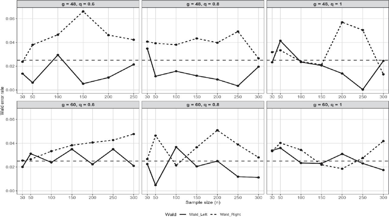
Figure 1 Estimated error probabilities of Wald test when $\mathrm{g}=48$ & $\mathrm{g}=60$.

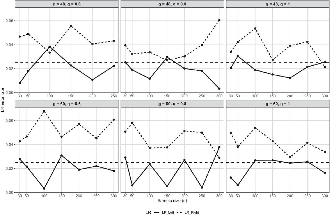
Figure 2 Estimated error probabilities of likelihood ratio test when $\mathrm{g}=48$ & $\mathrm{g}=60$.

In this section, the tooth data from a longitudinal perspective oral health study collected from the Signal Tandmobiel^® survey conducted in the Flanders region of Belgium between 1996 and 2001 were evaluated using the maximum likelihood method. Data were accessed in R using the mixAK package. The dataset Tandmob was loaded using the commands library(mixAK) and data(Tandmob). A cohort of 4468 randomly chosen children enrolled in the first year of basic education at the beginning children enrolled Derwent annual dental examinations by licensed dentists. We primarily considered the sample with size $\mathrm{n}=4,430$ because the remaining 38 sampled youngsters did not show up for any of the scheduled dental exams. The emergence times of 28 teeth, which are separated into seven different types, each of which has four teeth are the focus of this study. Permanent incisors (labels: 11, 21, 31, 41), permanent central canines (labels: 12, 22, 32, 42), permanent lateral canines (labels: 13, 23, 33, 43), permanent first premolars (labels: 14, 24, 34, 44), permanent second premolars (labels: 15, 25, 35, 45), permanent first molars (labels: 16, 26, 36, 46), and permanent second molars (labels: 17, 27, 37, 47). In the analysis that follows, we arrange these labels as $1,2,\mathrm{\dots },$ and 28. The emergence times of teeth 24, 26, and 46 were used as response variables. However, the dataset shows that emergence times suffer from DICD. Additionally, the absence of scheduled dental checks for the 38 children made it difficult to determine when their teeth would erupt, producing a skewed sample (Chen and Qiu 2023).

Table 6 Signal Tandmobiel^® data. Estimates and 95% confidence intervals for the emergence times

		Scale parameter ($\gamma$)			Shape Parameter ($\beta$)
Tooth	n	Estimate	95% CI	Estimate	95% CI
24	27	$-$3.41	[$-$6.35 $-$0.47]	3.83	[0.106 7.554]
26	4430	172.91	[123.71 222.11]	$-$135.81	[$-$232.046 $-$39.574]
46	127	0.6310	[0.3958 0.8662]	$-$2.45	[$-$4.7236 $-$0.1764]

Interpretation of Parameter Estimates and 95% Confidence Intervals

For Tooth 24, the scale parameter was significantly negative, and the relatively wide 95% confidence interval reflected substantial uncertainty, which was consistent with the small sample size. The shape parameter was significantly positive, indicating that the risk of tooth emergencies increased over time. The wide confidence interval suggests uncertainty regarding the rate at which this risk increases with age.

For Tooth 26, the scale parameter was large and significantly positive, implying a longer time to emergency compared with the other teeth. The confidence interval was relatively narrow, indicating high precision owing to the large sample size. The shape parameter was strongly negative, indicating that the risk of tooth emergence decreased over time. Despite its statistical significance, the extreme magnitude and wide confidence interval of the shape parameter may suggest potential model instability.

For Tooth 46, the scale parameter was significantly positive, suggesting a moderate timescale for the occurrence of emergencies. The confidence interval was reasonably narrow, indicating moderate precision. The shape parameter was significantly negative, indicating that the risk of emergency tooth extraction decreased over time, with the confidence interval suggesting a modest but clearly declining risk.

Overall, all parameters were statistically significant, as their 95% confidence intervals did not include zero. The scale parameters varied substantially across teeth, indicating meaningful differences in the timing of the emergencies. The shape parameters differed in sign, with Tooth 24 showing an increasing risk of emergency over time, whereas Teeth 26 and 46 showed decreasing risks over time.

Conclusion

The estimation procedure performed well for the Gompertz distribution under doubly interval-censored data, with bias, SE, and RMSE values remaining reasonably low. The results further indicated that bias, SE, and RMSE decreased as the study period, attendance probability, and sample size increased (Kiani and Arasan, 2013). Two confidence interval estimation methods the Wald and likelihood ratio approaches were examined. Overall, the Wald confidence intervals demonstrated superior performance compared to the likelihood ratio confidence intervals in the presence of doubly interval-censored data. This superior performance, particularly for large sample sizes, can be attributed to the asymptotic normality of the maximum likelihood estimators and the approximately quadratic nature of the log-likelihood function about the true parameter values. Under these conditions, the Wald and likelihood ratio confidence intervals become asymptotically equivalent. However, the Wald approach is computationally simpler and, in the simulation study, produced slightly shorter average interval lengths while maintaining coverage probabilities close to the nominal level (Loh et al., 2017; Kiani and Arasan, 2018). Consequently, the Wald confidence intervals exhibited better overall performance than the likelihood ratio confidence intervals. Future research could explore alternative parametric and nonparametric distributions, consider additional real-data applications, and extend the Gompertz model to incorporate extra parameters and covariate effects.

Acknowledgments

Data collection for the Signal Tandmobiel® project introduced in Section 5 was supported by Unilever, Belgium. The Signal Tandmobiel® project comprises the following partners: D. Declerck (Dental School, Catholic University Leuven), L. Martens (Dental School, University Ghent), J. Vanobbergen (Oral Health Promotion and Prevention, Flemish Dental Association), P. Bottenberg (Dental School, University Brussels), E. Lesaffre (Biostatistical Centre, Catholic University Leuven), and K. Hoppenbrouwers (Youth Health Department, Catholic University Leuven; Flemish Association for Youth Health Care).

Funding

The authors did not receive any specific funding for this work.

Declaration of Competing Interest

The corresponding author states that there are no competing interests.

Data Availability

This study used secondary data, available in open the domain; hence, it does not contain any primary data.

Ethical Approval

This study did not involve any studies conducted by the authors on humans or animals.

Consent to Participate

Not applicable.

Consent for Publication

Not applicable.

Clinical Trial Number

Not applicable.

References

[1] A. H. Peruski, B. Wu, L. Linley, K. P. Delaney, E. A. DiNenno, and A. S. Johnson, “Time from HIV infection to diagnosis in the U.S., 2014–2018,” IEEE Trans. Am. J. Prev. Med., vol. 61, no. 5, pp. 636–643, 2021, doi: 10.1016/j.amepre.2021.04.015.

[2] G. Pantaleo et al., “The qualitative nature of the primary immune response to HIV infection is a prognosticator of disease progression independent of the initial level of plasma viremia,” Proc. Natl. Acad. Sci. U.S.A., vol. 94, no. 1, pp. 254–258, 1997, doi: 10.1073/pnas.94.1.254.

[3] M. L. Calle, “The analysis of interval censoring and double censoring via Markov chain Monte Carlo methods,” Working document, Universitat de Vic, Vic, Spain, 2002.

[4] L. P. Chen and B. Qiu, “Analysis of length-biased and partly interval-censored survival data with mismeasured covariates,” Biometrics, vol. 79, no. 4, pp. 3929–3940, 2023, doi: 10.1093/biomtc/ujad117.

[5] K. Kiani and J. Arasan, “Gompertz model with time dependent covariate in the presence of interval-, right- and left-censored data,” J. Stat. Comput. Simul., vol. 83, no. 8, pp. 1472–1490, 2013, doi: 10.1080/00949655.2012.662979.

[6] Y. F. Loh, J. Arasan, H. Midi, and M. R. A. Bakar, “Inferential procedures for log logistic distribution with doubly interval-censored data,” J. Mod. Appl. Stat. Methods, vol. 16, no. 2, pp. 581–603, 2017, doi: 10.22237/jmasm/1509496320.

[7] K. Kiani and J. Arasan, “Survival model with doubly interval-censored data and timedependent covariates,” in Proc. World Congr. Eng., London, U.K., 2018, pp. 135–140.

[8] M. Z. Yin, Q. W. Zhu, and X. Lü, “Parameter estimation of the incubation period of COVID-19 based on the doubly interval-censored data model,” Nonlinear Dyn., vol. 106, no. 2, pp. 1347–1358, 2021, doi: 10.1007/s11071-021-06587-w.

[9] J. Sun, “Statistical analysis of doubly interval-censored failure time data,” in Handbook of Statistics: Advances in Survival Analysis, vol. 23. Amsterdam, The Netherlands: Elsevier, 2004, pp. 105–122, doi: 10.1016/S0169-7161(03)23006-6.

[10] W. Pan, “A multiple imputation approach to regression analysis for doubly censored data with application to AIDS studies,” Biometrics, vol. 57, no. 4, pp. 1245–1250, 2001, doi: 10.1111/j.0006-341X.2001.01245.x.

[11] V. De Gruttola and S. W. Lagakos, “The analysis of doubly censored data,” Biometrics, vol. 45, no. 1, pp. 1–11, 1989, doi: 10.2307/2532031.

[12] K. Kiani and J. Arasan, “Simulation of interval-censored data in medical and biological studies,” Int. J. Mod. Phys. Conf. Ser., vol. 9, pp. 112–118, 2012, doi: 10.1142/S2010194512005168.

[13] P. Bacchetti, “Estimating the incubation period of AIDS by comparing population infection and diagnosis patterns,” J. Amer. Stat. Assoc., vol. 85, no. 412, pp. 1002–1008, 1990, doi: 10.2307/2289596.

[14] Y. F. Loh, J. Arasan, H. Midi, and M. R. Abu Bakar, “A parametric model for doubly interval-censored lifetime data,” J. Sci. Technol., vol. 9, no. 2, 2017.

[15] J. Ramjith, C. Andolina, T. Bousema, and M. A. Jonker, “Flexible time-to-event models for double-interval-censored infectious disease data with clearance of the infection as a competing risk,” Front. Appl. Math. Stat., vol. 8, Art. no. 1035393, 2022, doi: 10.3389/fams.2022.1035393.

[16] J. Kim, Y.-J. Kim, and C. M. Nam, “A generalized log-rank-type test for comparing survivals with doubly interval-censored data,” Biom. J., vol. 51, no. 4, pp. 689–696, 2009, doi: 10.1002/bimj.200800253.

[17] M. Y. Kim, V. De Gruttola, and S. W. Lagakos, “Analyzing doubly censored data with covariates, with application to AIDS,” Biometrics, vol. 49, no. 1, pp. 13–22, Mar. 1993.

[18] N. G. Reich, J. Lessler, D. A. T. Cummings, and R. Brookmeyer, “Estimating incubation period distributions with coarse data,” Statistics in Medicine, vol. 28, no. 22, pp. 2769–2784, 2009, doi: 10.1002/sim.3659.

[19] R. Oller, G. Gómez, and M. L. Calle, “Interval censoring: Model characterizations for the validity of the simplified likelihood,” Canadian Journal of Statistics, vol. 32, no. 3, pp. 315–326, 2004.

[20] K. Sruthi and M. Kumar, “Fuzzy reliability estimation within a stress-strength framework incorporating distortion functions,” Journal of Reliability and Statistical Studies, vol. 19, no. 1, pp. 3–24, 2026, doi: 10.13052/jrss0974-8024.1913.

BIOGRAPHIES

Himani Kotian received the bachelor’s degree in Statistics from Mangalore University in 2013, the master’s degree in Biostatistics from Manipal University in 2015, and Pursuing philosophy of doctorate degree in Survival Analysis (Doubly Interval-Censored Data) from Manipal University, respectively. She is currently working as a Lecturer cum Biostatistician in the Department of Community Medicine, Kasturba Medical College Mangalore. Her research areas include Inferential Statistics, Survival analysis, and Machine Learning Technique.

Sunita Sharma is an Assistant Professor in the Department of Mathematics at Manipal Institute of Technology, Manipal, Karnataka, India. She obtained her Ph.D. in Statistics from G. B. Pant University of Agriculture and Technology, Pantnagar, Uttarakhand, India.

Her research interests include Bayesian Statistics, Reliability Engineering, Statistical Inference, and Applied Probability. Dr. Sharma has published numerous research articles in reputed international journals indexed in SCI and Scopus databases. Her research primarily focuses on reliability analysis, Bayesian estimation, and stochastic modeling of complex systems.

In addition to her research contributions, Dr. Sharma actively serves as a reviewer for several national and international journals in Statistics, Reliability Engineering, and related disciplines.

Asha Kamath is Associate Director and Professor of Department of Data Science, PSPH, Manipal Academy of Higher Education (MAHE), Manipal. Dr. Kamath is an expert in research methodology and biostatistics. She regularly undertakes statistical consultancy for medical researchers and supervises research among medical postgraduates. She is a panel member on the PhD committee of MAHE. Dr. Kamath has worked extensively in the designing and analysis of epidemiological studies, clinical trials, model building, Bayesian analysis, Time series analysis of health and climate data, and allied health fields such as adolescent health and geriatrics. She has been a part of several collaborations, both nationally and internationally and has been an investigator/co-investigator on several projects for ICMR and other reputed institutions grant from the University of Alabama at Birmingham International Training and Research in Environmental and Occupational Health program from the National Institutes of Health-Fogarty International Center (NIH-FIC) for developing R manual for time series analysis.

She is a Life member of the Indian Society for Medical Statistics (ISMS). Dr Kamath has published more than 175 articles in national and international journals which have been indexed in SCOPUS and PubMed databases. She has written six chapters in books and has served as a resource person in workshops as a research methodologist as well as a statistician.

Vasudeva Guddattu is a Professor in the Department of Applied Statistics and Data Science of Public Health at Manipal Academy of Higher Education. He is Coordinator for MSc Biostatistics Program. Professor Guddattu obtained his master’s degree in Statistics from Mangalore University in 2005 and completed his PhD in Count Data Regression from the same university in 2014. His areas of expertise encompass categorical data analysis, discrete data modelling, biostatistics, and statistical methods for health research. He is a distinguished researcher with an h-index of 23 and has made significant contributions to scientific literature through numerous publications, including randomized controlled trials and mixed-methods studies. His research has contributed substantially to advancing statistical applications in medical and public health research.

Journal of Reliability and Statistical Studies, Vol. 19, Issue 2 (2026), 635–664
doi: 10.13052/jrss0974-8024.19216
© 2026 River Publishers