Reliability Analysis of Complex System by Intuitionistic Fuzzy Set and ML Approach
Deepanshi1, Akansha Gupta2 and Nupur Goyal1,*
1Department of Mathematics, Graphic Era (Deemed to be University), Dehradun, India
2Department of Computer Science and Engineering, Graphic Era (Deemed to be University), Dehradun, India
E-mail: chauhandeepanshi86@gmail.com; akanshagupta.cse@geu.ac.in; nupurgoyalgeu@gmail.com
*Corresponding Author
Received 27 May 2026; Accepted 25 September 2026
Abstract
Reliability analysis of complex systems is important for the purpose of ensuring efficient and safe operation in contemporary engineering applications. This study presents a hybrid approach to analyse the reliability of complex systems by Fault Tree Analysis (FTA) with intuitionistic fuzzy sets, under the consideration of Weibull distribution to express uncertainty in system failure. To make the analysis more comprehensive, machine learning (ML) algorithms such as Linear Regression, Decision Trees, Random Forests, Support Vector Regression, K-Nearest Neighbors, and neural networks (MLP and DNN) are used to predict the system reliability. The ML models are tested on the basis of values and results are also plotted using bar plots so that the performance of the models with different datasets can be explained clearly. The Decision Tree and Random Forest models achieved excellent predictive accuracy with R square value 99.9995%. This study helps engineers effectively handle uncertainty in complex systems, make accurate failure predictions, and develop optimized maintenance strategies.
Keywords: FTA, reliability, fuzzy intuitionistic sets, ML algorithms, R2 score.
1 Introduction
In modern scenario engineering systems such as aerospace vehicles, power generation units, drone delivery systems, and automated manufacturing lines have become very complex and interconnected. This complexity has made their reliable operation very critical, because if even a single component fails, the performance of the entire system can be impacted. For this reason, system reliability analysis is very important so that the behaviour of each component can be accurately assessed. In real-life situations, systems often fail due to unstable power supply or varying conditions. When system reliability increases, production efficiency and cost-effectiveness also improve-especially in the manufacturing, power plants, and industrial automation sectors. Maintaining high reliability is a fundamental requirement of every system’s design and operation. In this context, the study of repairable systems also plays an important role, because the repairman’s skills and decision-making actions directly impact the system’s overall reliability and economics.
Fault Tree Analysis (FTA) is a well-known technique used to visualize and analyse system failures that affect the reliability. Suresh et al. FTA follows a top-down hierarchical structure, breaking down top events into basic component-level failures using logical “AND” and “OR” gates [1]. However, the problem with traditional FTA is that it relies on crisp data meaning the exact failure probability of each event must be defined. In real-world cases, this data is incomplete, uncertain, or based on expert opinion, which inherently introduces vagueness. Because of this, the accuracy and capability of traditional FTA is limited in handling uncertainty. Fuzzification provides an effective solution to overcome this limitation. Fuzzification converts crisp values into fuzzy sets, where probability is represented as a range rather than a single value.
In today’s digital and data-driven industrial environment, not only handling uncertainty is important, but intelligent prediction and performance optimization are equally crucial. ML techniques are helpful to overcome this situation. Many algorithms like ANN, SVM, Decision Tree etc. use historical system data to find patterns in component failure and predict future occurrences. Particularly when analysing large-scale system and dynamic operating situations, these techniques are more effective than traditional reliability analysis.
The structure of this paper is as follows: Section 2 provides the literature relevant to this study. The model details like notations, system description and block diagram of complex system provide in Section 3 there are mathematical modelling in Section 4. The proposed methodology numerically explained in Section 5. System performance by ML models is presented in Section 6. Hyper parameter discussed in Section 7. Statistical study of ML model is done in Section 8. Conclusion is provided in Section 9.
The key contributions of this study are given below:
• Development of a fuzzy FTA-based reliability modelling.
• Defuzzification of membership and non-membership reliability measure.
• Construction of structured reliability datasets for predictive modelling.
• Comparative evaluation of multiple ML algorithms.
2 Literature Review
In past, a lot of research have been studied many techniques like Markov process, Bayesian network, Monte Carle-based simulation etc. for reliability analysis. Wang et al. proposed new reliability importance indices for repairable systems using RBD-based simulation, addressing the limitations of traditional analytical approaches [2]. Extending the application of RBD and simulation techniques, Soleimani and Pourgol-Mohammad incorporated Monte Carlo simulation to evaluate the reliability of horizontal drilling equipment during the early design phase, particularly under limited failure data conditions [3]. Building upon simulation-based frameworks, Mi et al. integrated Dynamic Fault Tree (DFT), Bayesian Networks (BN), and Monte Carlo simulation to assess electromechanical systems under uncertainty, further strengthening the analysis through extended P-Box modelling for incomplete data [4]. In a similar direction of enhancing probabilistic modelling, Torres-Toledano et al. transformed RBDs into Bayesian Networks and computed system reliability through probability propagation, thereby improving modelling flexibility. Complementing these probabilistic approaches [5], Dhillon and Rayapati focused on three-state device systems and analysed the influence of open and short failures on bridge network reliability. At the conceptual level [6], Juang et al. emphasized that system performance is strongly governed by internal logical structure and component failure behaviour [7]. This structural understanding aligns with the classification provided by Tyagi et al. who further clarified the definition of repairable systems [8]. Applying these theoretical foundations, Shivani et al. used a Markov process to analyse a complex series-parallel repairable system under different repair distributions [9]. Finally, Tekiner-Mogulkoc and Coit extended reliability analysis toward optimization by proposing exact and heuristic algorithms to minimize the coefficient of variation of system reliability under uncertainty [10].
Reliability development is influenced by cost-related factors such as system complexity, quality demands, regulations, government standards, and failures or warranties. Hryniewicz introduced fuzzy and shadowed sets to estimate reliability under vague lifetime data without complex computations, while Poonia et al. assist the reliability and availability of warm standby repairable computer network system [11, 12]. Wu et al. further enhanced FTA by integrating fuzzy reasoning Petri nets with improved fault identification techniques such as final truth degree and cosine matching functions [13]. More recently, Kaushik and Kumar developed intuitionistic fuzzy FTA models using triangular intuitionistic fuzzy numbers (TIFN) and expert judgment aggregation, validating them through practical case studies [14, 15]. Additionally, Bai applied FTA for network equipment fault detection [16], and Zacchaeus et al. examined safety risks in the oil and gas sector, proposing mitigation strategies. Collectively, these studies reflect the evolution of fuzzy and intuitionistic fuzzy FTA approaches for enhanced reliability and risk assessment under uncertainty [17]. Samal and Raj proposed a software reliability growth model incorporating fault removal efficiency and an S-shaped fault detection function within a non-homogeneous Poisson process. The model was validated using software testing data and compared with existing models [34]. Samal and Kumar proposed software reliability growth models incorporating tester fatigue, S-shaped learning curves, and fault interdependencies to represent human errors more realistically. The models were evaluated using MSE, MAE, and on two failure datasets, demonstrating improved software reliability assessment [35].
Researchers have found that ML regression techniques such as LR, DT, RF, SVR, KNN, and neural networks (NN) are effective in accurately predicting the performance of complex systems. Furthermore, Cao and Bai introduced a DNN-based surrogate modelling approach integrated with fuzzy optimization for aero engine design, achieving high accuracy and approximately 99.997% faster results compared to Monte Carlo simulation [18]. Hasan et al. used decision tree algorithms in WEKA and found Random Forest most accurate for predicting student performance [19], while Olaniyi et al. reported BF Tree as the best classifier with 67.07% accuracy [20]. In regression-based studies, Joseph et al. linked processor performance to architectural parameters using linear regression with AIC [21], and Ciulla and D’Amico developed a simplified linear regression model to estimate building energy demand based on parametric simulations [22]. Al-Shehri et al. compared SVM and KNN for predicting students’ final exam performance and found that SVM slightly outperformed KNN with a correlation coefficient of 0.96 [23]. Extending this idea, Dewi and Chen combined Random Forest-based feature selection with tuned SVM regression, achieving improved accuracy through lower RMSE and higher R-values [24]. Similarly, Bansal et al. reviewed major ML algorithms and concluded that SVM and LSTM are among the most robust and accurate methods for real-world predictive analytics [25]. Samal and Shukla proposed a stacked regression framework integrating traditional ML models with an RNN meta-learner was proposed for accurate software fault prediction. The approach demonstrated improved performance over individual learners in terms of RMSE and MAE across three real-world datasets [36]. Table 1 provides key references for the comparative study of literature.
Table 1 Comparative study of literature
| Reference | Reliability | FTA | IFS | ML Models |
| Mi et al. [4] | X | X | ||
| Dhillon & Rayapati [6] | X | X | X | |
| Torres-Toledano [5] | X | X | X | |
| Shivani et al. [9] | X | X | X | |
| Wu et al. [13] | X | |||
| Suresh et al. [12] | X | |||
| Kaushik & Kumar [15] | X | |||
| Bai [16] | X | X | X | |
| Zacchaeus et al. [17] | X | X | X | |
| Olaniyi et al. [20] | X | X | X | |
| Joseph et al. [21] | X | X | X | |
| Ciulla & D’Amico [22] | X | X | X | |
| Al-Shehri et al. [23] | X | X | X | |
| Dewi & Chen [24] | X | X | X | |
| Bansal et al. [25] | X | X | X | |
| Proposed Study |
There are various limitations of the existing reliability models like Markov approach and Universal Generating Function (UGF) used for complex systems. Exponential failure and repair time distributions, along with the memoryless property, may not always be suitable for real-world systems. Additionally, the number of states grows quickly as the complexity of the system grows. Likewise, UGF methods need the explicit state of the components and accurate probabilistic data. To overcome these limitations, the proposed FTA-IFS-ML framework systematically identifies failure mechanisms through FTA, represents uncertainty using membership and non-membership information in IFS, and evaluated prediction accuracy and the suitable model for reliable system reliability evaluation by ML models.
Hence, the study proposed the following key research questions:
RQ.1. How to detect the reliability of complex system?
RQ.2. How can the performance of a system be precisely assessed?
RQ.3. How to determine the most suitable ML model for predicting system performance?
3 Model Details
3.1 Notations
The following is a list of the notations related to the work:
| Probability of system failure | |
| , , | Probability of failure of subsystem |
| respectively. | |
| Reliability of the system. | |
| Component’s Reliability | |
 |
System |
 |
Sub-system |
 |
AND Gate |
 |
OR Gate |
3.2 System Description
To examine the performance of the complex system, understanding its basic configuration is crucial. The reliability block diagram shows linked blocks set up in parallel and series arrangements. The four subsystems that make up this system are A, B, C, D, and E. These subsystems are connected in series, with subsystem A being made up of two parallel components, A1 and A2. Additionally, they are both connected in series to the same component, A3. In contrast, subsystem B consists of three parts, B1, B2, and B3, which are placed in series. Subsystem C, on the other hand, is made up of two parallel components, C1 and C2. Furthermore, they are both connected to the same component, C3 in series. While sub-system having three components, and that arranged in parallel. While subsystem having two components, , and that arranged in series. Autonomous Drone Delivery Systems (ADDS), power system and flight control system are real-world example of this type of system. The block diagram of system configuration is displayed in Figure 1.

Figure 1 System Reliability Block diagram.
The fault tree of the complex system (Figure 1) is designed by considering various failure mode such as hardware failure, human error, or environmental factors, and represented in Figure 2. Figure 3 explains the complete methodology step by step.
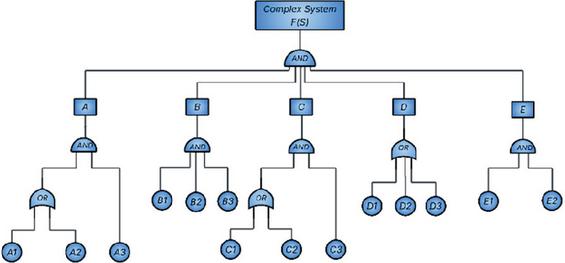
Figure 2 Structure of FTA.
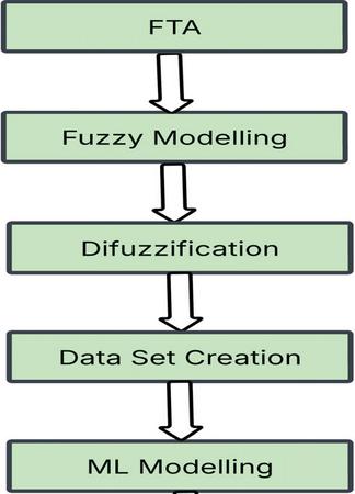
Figure 3 Flow Chart of Methodology.
4 Mathematical Modelling of the Complex System
4.1 Reliability Formulation by FTA
Fault tree model for a given complex system is constructed as to derive the equation of reliability.
After the simplification of above equations, we get the component’s probabilities as
Where, is the th component’s reliability. The designed system reliability by fault tree analysis is
| (1) |
If the components follow identical independent distribution, then and the resultant reliability is obtained as
| (2) |
4.2 Fuzzy Reliability by TIFN
4.2.1 Intuitionistic fuzzy sets
The definition of an IFS, in is an object that fits the form [26, 27].
Where,
For TIFN,
The physical interpretation five parameters () of the TIFN is as follows: () and represent the lower and upper limits of the possible reliability. The parameters and represent the inner lower and upper boundaries associated with the membership and non-membership information. The parameter denotes the most representative or central reliability value. Thus, these five parameters collectively represent the possible reliability range and the associated uncertainty in the reliability assessment.
Where
Its membership and non-membership function are defined as,
| (3) | ||
| (4) |
By applying the Weibull distribution, the component reliability is obtained as
| (5) |
Where,
Where is the spread, is the Weibull slope. By varying the slope value, this distribution can simulate a wide range of lifetime data.
5 Numerical Illustration
Assuming that (2.5, 2.75, 2.85, 2.95, 3), is a TIFN, that are used to determine the membership and non-membership values. Hence, -cut and -cut of intuitionistic fuzzy set are obtained as, and . The membership and non-membership degrees satisfy hence, and represents the non-membership degree in Equations (14) and (15).
Using -cut and -cut the fuzzy reliability can be obtained as:
| (6) | ||
| (7) | ||
| (8) | ||
| (9) |
The values of -cut and -cut of the fuzzy reliability are obtained as shown in Table 2. By taking at time , at interval , and , at interval 0.1.
Table 2 Sample of fuzzy reliability
| Time (t) | Time (t) | ||||||
| 0 | 0 | (1.0000, 1.0000) | (1.0000, 1.0000) | 10 | 0.5 | (0.6977, 0.7111) | (0.6799, 0.7143) |
| 0 | 0.1 | (1.0000, 1.0000) | (1.0000, 1.0000) | 10 | 0.6 | (0.6991, 0.7098) | (0.6850, 0.7124) |
| 0 | 0.2 | (1.0000, 1.0000) | (1.0000, 1.0000) | 10 | 0.7 | (0.7004, 0.7085) | (0.6900, 0.7104) |
| 0 | 0.3 | (1.0000, 1.0000) | (1.0000, 1.0000) | 10 | 0.8 | (0.7018, 0.7071) | (0.6949, 0.7085) |
| 0 | 0.4 | (1.0000, 1.0000) | (1.0000, 1.0000) | 10 | 0.9 | (0.7031, 0.7058) | (0.6998, 0.7065) |
| 0 | 0.5 | (1.0000, 1.0000) | (1.0000, 1.0000) | 10 | 1.0 | (0.7045, 0.7045) | (0.7045, 0.7045) |
| 0 | 0.6 | (1.0000, 1.0000) | (1.0000, 1.0000) | 12 | 0 | (0.6164, 0.6457) | (0.5754, 0.6526) |
| 0 | 0.7 | (1.0000, 1.0000) | (1.0000, 1.0000) | 12 | 0.1 | (0.6179, 0.6443) | (0.5814, 0.6506) |
| 0 | 0.8 | (1.0000, 1.0000) | (1.0000, 1.0000) | 12 | 0.2 | (0.6194, 0.6429) | (0.5874, 0.6485) |
| 0 | 0.9 | (1.0000, 1.0000) | (1.0000, 1.0000) | 12 | 0.3 | (0.6210, 0.6415) | (0.5932, 0.6464) |
| 0 | 1.0 | (1.0000, 1.0000) | (1.0000, 1.0000) | 12 | 0.4 | (0.6225, 0.6401) | (0.5990, 0.6443) |
| 2 | 0 | (0.9873, 0.9896) | (0.9837, 0.9900) | 12 | 0.5 | (0.6240, 0.6387) | (0.6046, 0.6422) |
| 2 | 0.1 | (0.9875, 0.9895) | (0.9843, 0.9899) | 12 | 0.6 | (0.6255, 0.6372) | (0.6101, 0.6401) |
| 2 | 0.2 | (0.9876, 0.9894) | (0.9848, 0.9898) | 12 | 0.7 | (0.6270, 0.6358) | (0.6156, 0.6379) |
| 2 | 0.3 | (0.9877, 0.9893) | (0.9854, 0.9896) | 12 | 0.8 | (0.6285, 0.6343) | (0.6210, 0.6358) |
| 2 | 0.4 | (0.9878, 0.9892) | (0.9859, 0.9895) | 12 | 0.9 | (0.6299, 0.6329) | (0.6262, 0.6336) |
| 2 | 0.5 | (0.9880, 0.9891) | (0.9864, 0.9893) | 12 | 1.0 | (0.6314, 0.6314) | (0.6314, 0.6314) |
| 2 | 0.6 | (0.9881, 0.9890) | (0.9868, 0.9892) | 14 | 0 | (0.5496, 0.5803) | (0.5074, 0.5876) |
| 2 | 0.7 | (0.9882, 0.9888) | (0.9873, 0.9890) | 14 | 0.1 | (0.5512, 0.5789) | (0.5136, 0.5855) |
| 2 | 0.8 | (0.9883, 0.9887) | (0.9877, 0.9888) | 14 | 0.2 | (0.5528, 0.5774) | (0.5197, 0.5833) |
| 2 | 0.9 | (0.9884, 0.9886) | (0.9881, 0.9887) | 14 | 0.3 | (0.5544, 0.5759) | (0.5257, 0.5811) |
| 2 | 1.0 | (0.9885, 0.9885) | (0.9885, 0.9885) | 14 | 0.4 | (0.5560, 0.5744) | (0.5316, 0.5789) |
| 4 | 0 | (0.9332, 0.9424) | (0.9188, 0.9445) | 14 | 0.5 | (0.5575, 0.5729) | (0.5374, 0.5766) |
| 4 | 0.1 | (0.9337, 0.9420) | (0.9210, 0.9439) | 14 | 0.6 | (0.5591, 0.5714) | (0.5432, 0.5744) |
| 4 | 0.2 | (0.9342, 0.9416) | (0.9232, 0.9433) | 14 | 0.7 | (0.5607, 0.5699) | (0.5488, 0.5722) |
| 4 | 0.3 | (0.9347, 0.9411) | (0.9252, 0.9426) | 14 | 0.8 | (0.5622, 0.5684) | (0.5544, 0.5699) |
| 4 | 0.4 | (0.9352, 0.9407) | (0.9273, 0.9420) | 14 | 0.9 | (0.5638, 0.5668) | (0.5599, 0.5676) |
| 4 | 0.5 | (0.9356, 0.9403) | (0.9292, 0.9414) | 14 | 1.0 | (0.5653, 0.5653) | (0.5653, 0.5653) |
| 4 | 0.6 | (0.9361, 0.9398) | (0.9311, 0.9407) | 16 | 0 | (0.4904, 0.5216) | (0.4481, 0.5291) |
| 4 | 0.7 | (0.9366, 0.9394) | (0.9329, 0.9400) | 16 | 0.1 | (0.4920, 0.5201) | (0.4543, 0.5269) |
| 4 | 0.8 | (0.9371, 0.9389) | (0.9347, 0.9394) | 16 | 0.2 | (0.4936, 0.5186) | (0.4603, 0.5246) |
| 4 | 0.9 | (0.9375, 0.9385) | (0.9364, 0.9387) | 16 | 0.3 | (0.4952, 0.5171) | (0.4663, 0.5224) |
| 4 | 1.0 | (0.9380, 0.9380) | (0.9380, 0.9380) | 16 | 0.4 | (0.4968, 0.5156) | (0.4723, 0.5201) |
| 6 | 0 | (0.8553, 0.8720) | (0.8303, 0.8758) | 16 | 0.5 | (0.4984, 0.5140) | (0.4781, 0.5178) |
| 6 | 0.1 | (0.8562, 0.8713) | (0.8341, 0.8747) | 16 | 0.6 | (0.5000, 0.5125) | (0.4839, 0.5156) |
| 6 | 0.2 | (0.8571, 0.8705) | (0.8378, 0.8736) | 16 | 0.7 | (0.5016, 0.5110) | (0.4896, 0.5133) |
| 6 | 0.3 | (0.8580, 0.8697) | (0.8414, 0.8724) | 16 | 0.8 | (0.5032, 0.5094) | (0.4952, 0.5110) |
| 6 | 0.4 | (0.8589, 0.8689) | (0.8449, 0.8713) | 16 | 0.9 | (0.5047, 0.5079) | (0.5008, 0.5086) |
| 6 | 0.5 | (0.8597, 0.8681) | (0.8483, 0.8701) | 16 | 1.0 | (0.5063, 0.5063) | (0.5063, 0.5063) |
| 6 | 0.6 | (0.8606, 0.8673) | (0.8516, 0.8689) | 18 | 0 | (0.4382, 0.4693) | (0.3966, 0.4767) |
| 6 | 0.7 | (0.8615, 0.8665) | (0.8549, 0.8677) | 18 | 0.1 | (0.4398, 0.4678) | (0.4026, 0.4745) |
| 6 | 0.8 | (0.8623, 0.8657) | (0.8580, 0.8665) | 18 | 0.2 | (0.4414, 0.4662) | (0.4086, 0.4723) |
| 6 | 0.9 | (0.8632, 0.8648) | (0.8610, 0.8652) | 18 | 0.3 | (0.4430, 0.4647) | (0.4145, 0.4700) |
| 6 | 1.0 | (0.8640, 0.8640) | (0.8640, 0.8640) | 18 | 0.4 | (0.4446, 0.4632) | (0.4203, 0.4678) |
| 8 | 0 | (0.7716, 0.7942) | (0.7386, 0.7994) | 18 | 0.5 | (0.4462, 0.4617) | (0.4261, 0.4655) |
| 8 | 0.1 | (0.7728, 0.7932) | (0.7436, 0.7979) | 18 | 0.6 | (0.4477, 0.4602) | (0.4318, 0.4632) |
| 8 | 0.2 | (0.7740, 0.7921) | (0.7484, 0.7963) | 18 | 0.7 | (0.4493, 0.4586) | (0.4374, 0.4609) |
| 8 | 0.3 | (0.7752, 0.7910) | (0.7531, 0.7948) | 18 | 0.8 | (0.4509, 0.4571) | (0.4430, 0.4586) |
| 8 | 0.4 | (0.7763, 0.7899) | (0.7577, 0.7932) | 18 | 0.9 | (0.4524, 0.4555) | (0.4485, 0.4563) |
| 8 | 0.5 | (0.7775, 0.7888) | (0.7623, 0.7916) | 18 | 1.0 | (0.4540, 0.4540) | (0.4540, 0.4540) |
| 8 | 0.6 | (0.7787, 0.7877) | (0.7667, 0.7899) | 20 | 0 | (0.4540, 0.4540) | (0.3519, 0.4301) |
| 8 | 0.7 | (0.7798, 0.7866) | (0.7710, 0.7883) | 20 | 0.1 | (0.3938, 0.4213) | (0.3577, 0.4279) |
| 8 | 0.8 | (0.7810, 0.7855) | (0.7752, 0.7866) | 20 | 0.2 | (0.3954, 0.4198) | (0.3634, 0.4257) |
| 8 | 0.9 | (0.7821, 0.7844) | (0.7793, 0.7850) | 20 | 0.3 | (0.3969, 0.4183) | (0.3692, 0.4235) |
| 8 | 1.0 | (0.7833, 0.7833) | (0.7833, 0.7833) | 20 | 0.4 | (0.3985, 0.4168) | (0.3748, 0.4213) |
| 10 | 0 | (0.6907, 0.7175) | (0.6526, 0.7237) | 20 | 0.5 | (0.4000, 0.4153) | (0.3804, 0.4190) |
| 10 | 0.1 | (0.6921, 0.7162) | (0.6583, 0.7219) | 20 | 0.6 | (0.4016, 0.4138) | (0.3860, 0.4168) |
| 10 | 0.2 | (0.6935, 0.7150) | (0.6638, 0.7200) | 20 | 0.7 | (0.4031, 0.4123) | (0.3915, 0.4145) |
| 10 | 0.3 | (0.6949, 0.7137) | (0.6693, 0.7181) | 20 | 0.8 | (0.4047, 0.4108) | (0.3969, 0.4123) |
| 10 | 0.4 | (0.6963, 0.7124) | (0.6746, 0.7162) | 20 | 0.9 | (0.4062, 0.4092) | (0.4024, 0.4100) |
| 10 | 0.5 | (0.6977, 0.7111) | (0.6799, 0.7143) | 20 | 1.0 | (0.4077, 0.4077) | (0.4077, 0.4077) |
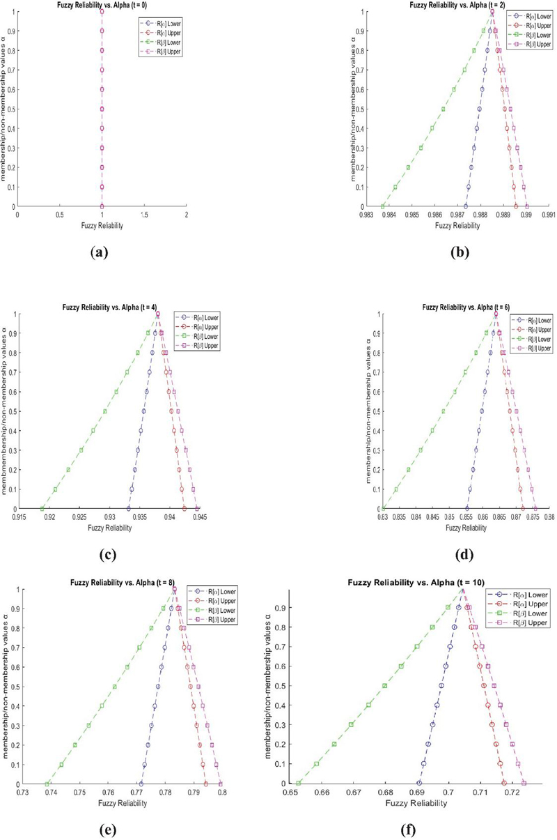
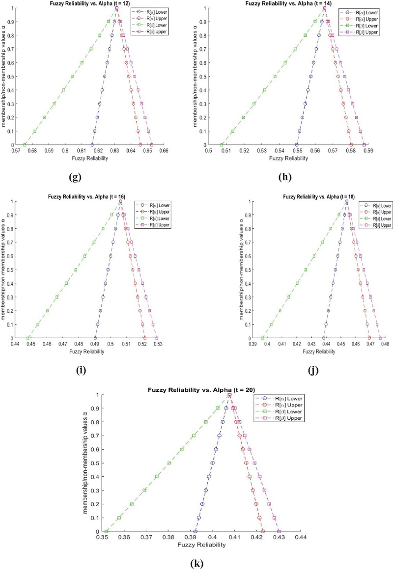
Figure 4 (a) to (k): Fuzzy Reliability vs. at to 20.
For further analysis, we converted the uncertain or vague results obtained from fuzzy systems into crisp numerical values of -cut & -cut through a defuzzification process as given in Table 3.
Table 3 Defuzzzified -cut & -cut values
| Time (t) | Time (t) | ||||||
| 0 | 0 | 1.0000 | 1.0000 | 10 | 0.5 | 0.7044 | 0.6971 |
| 0 | 0.1 | 1.0000 | 1.0000 | 10 | 0.6 | 0.7044 | 0.6987 |
| 0 | 0.2 | 1.0000 | 1.0000 | 10 | 0.7 | 0.7045 | 0.7002 |
| 0 | 0.3 | 1.0000 | 1.0000 | 10 | 0.8 | 0.7045 | 0.7017 |
| 0 | 0.4 | 1.0000 | 1.0000 | 10 | 0.9 | 0.7045 | 0.7031 |
| 0 | 0.5 | 1.0000 | 1.0000 | 10 | 1.0 | 0.7045 | 0.7045 |
| 0 | 0.6 | 1.0000 | 1.0000 | 12 | 0 | 0.6310 | 0.6140 |
| 0 | 0.7 | 1.0000 | 1.0000 | 12 | 0.1 | 0.6311 | 0.6160 |
| 0 | 0.8 | 1.0000 | 1.0000 | 12 | 0.2 | 0.6312 | 0.6179 |
| 0 | 0.9 | 1.0000 | 1.0000 | 12 | 0.3 | 0.6312 | 0.6198 |
| 0 | 1.0 | 1.0000 | 1.0000 | 12 | 0.4 | 0.6313 | 0.6216 |
| 2 | 0 | 0.9885 | 0.9869 | 12 | 0.5 | 0.6313 | 0.6234 |
| 2 | 0.1 | 0.9885 | 0.9871 | 12 | 0.6 | 0.6313 | 0.6251 |
| 2 | 0.2 | 0.9885 | 0.9873 | 12 | 0.7 | 0.6314 | 0.6268 |
| 2 | 0.3 | 0.9885 | 0.9875 | 12 | 0.8 | 0.6314 | 0.6284 |
| 2 | 0.4 | 0.9885 | 0.9877 | 12 | 0.9 | 0.6314 | 0.6299 |
| 2 | 0.5 | 0.9885 | 0.9878 | 12 | 1.0 | 0.6314 | 0.6314 |
| 2 | 0.6 | 0.9885 | 0.9880 | 14 | 0 | 0.5650 | 0.5475 |
| 2 | 0.7 | 0.9885 | 0.9881 | 14 | 0.1 | 0.5650 | 0.5495 |
| 2 | 0.8 | 0.9885 | 0.9883 | 14 | 0.2 | 0.5651 | 0.5515 |
| 2 | 0.9 | 0.9885 | 0.9884 | 14 | 0.3 | 0.5651 | 0.5534 |
| 2 | 1.0 | 0.9885 | 0.9885 | 14 | 0.4 | 0.5652 | 0.5552 |
| 4 | 0 | 0.9378 | 0.9316 | 14 | 0.5 | 0.5652 | 0.5570 |
| 4 | 0.1 | 0.9378 | 0.9324 | 14 | 0.6 | 0.5653 | 0.5588 |
| 4 | 0.2 | 0.9379 | 0.9332 | 14 | 0.7 | 0.5653 | 0.5605 |
| 4 | 0.3 | 0.9379 | 0.9339 | 14 | 0.8 | 0.5653 | 0.5621 |
| 4 | 0.4 | 0.9379 | 0.9346 | 14 | 0.9 | 0.5653 | 0.5637 |
| 4 | 0.5 | 0.9380 | 0.9353 | 14 | 1.0 | 0.5653 | 0.5653 |
| 4 | 0.6 | 0.9380 | 0.9359 | 16 | 0 | 0.5060 | 0.4886 |
| 4 | 0.7 | 0.9380 | 0.9365 | 16 | 0.1 | 0.5061 | 0.4906 |
| 4 | 0.8 | 0.9380 | 0.9370 | 16 | 0.2 | 0.5061 | 0.4925 |
| 4 | 0.9 | 0.9380 | 0.9375 | 16 | 0.3 | 0.5062 | 0.4944 |
| 4 | 1.0 | 0.9380 | 0.9380 | 16 | 0.4 | 0.5062 | 0.4962 |
| 6 | 0 | 0.8637 | 0.8530 | 16 | 0.5 | 0.5062 | 0.4980 |
| 6 | 0.1 | 0.8637 | 0.8544 | 16 | 0.6 | 0.5063 | 0.4997 |
| 6 | 0.2 | 0.8638 | 0.8557 | 16 | 0.7 | 0.5063 | 0.5014 |
| 6 | 0.3 | 0.8638 | 0.8569 | 16 | 0.8 | 0.5063 | 0.5031 |
| 6 | 0.4 | 0.8639 | 0.8581 | 16 | 0.9 | 0.5063 | 0.5047 |
| 6 | 0.5 | 0.8639 | 0.8592 | 16 | 1.0 | 0.5063 | 0.5063 |
| 6 | 0.6 | 0.8639 | 0.8603 | 18 | 0 | 0.4537 | 0.4367 |
| 6 | 0.7 | 0.8640 | 0.8613 | 18 | 0.1 | 0.4538 | 0.4386 |
| 6 | 0.8 | 0.8640 | 0.8622 | 18 | 0.2 | 0.4538 | 0.4404 |
| 6 | 0.9 | 0.8640 | 0.8631 | 18 | 0.3 | 0.4539 | 0.4422 |
| 6 | 1.0 | 0.8640 | 0.8640 | 18 | 0.4 | 0.4539 | 0.4440 |
| 8 | 0 | 0.7829 | 0.7690 | 18 | 0.5 | 0.4539 | 0.4458 |
| 8 | 0.1 | 0.7830 | 0.7707 | 18 | 0.6 | 0.4539 | 0.4475 |
| 8 | 0.2 | 0.7830 | 0.7724 | 18 | 0.7 | 0.4540 | 0.4492 |
| 8 | 0.3 | 0.7831 | 0.7739 | 18 | 0.8 | 0.4540 | 0.4508 |
| 8 | 0.4 | 0.7831 | 0.7755 | 18 | 0.9 | 0.4540 | 0.4524 |
| 8 | 0.5 | 0.7832 | 0.7769 | 18 | 1.0 | 0.4540 | 0.4540 |
| 8 | 0.6 | 0.7832 | 0.7783 | 20 | 0 | 0.4075 | 0.3910 |
| 8 | 0.7 | 0.7832 | 0.7796 | 20 | 0.1 | 0.4076 | 0.3928 |
| 8 | 0.8 | 0.7833 | 0.7809 | 20 | 0.2 | 0.4076 | 0.3946 |
| 8 | 0.9 | 0.7833 | 0.7821 | 20 | 0.3 | 0.4076 | 0.3963 |
| 8 | 1.0 | 0.7833 | 0.7833 | 20 | 0.4 | 0.4076 | 0.3980 |
| 10 | 0 | 0.7041 | 0.6882 | 20 | 0.5 | 0.4077 | 0.3997 |
| 10 | 0.1 | 0.7042 | 0.6901 | 20 | 0.6 | 0.4077 | 0.4014 |
| 10 | 0.2 | 0.7042 | 0.6919 | 20 | 0.7 | 0.4077 | 0.403 |
| 10 | 0.3 | 0.7043 | 0.6937 | 20 | 0.8 | 0.4077 | 0.4046 |
| 10 | 0.4 | 0.7044 | 0.6954 | 20 | 0.9 | 0.4077 | 0.4062 |
| 10 | 0.5 | 0.7044 | 0.6971 | 20 | 1.0 | 0.4077 | 0.4077 |
Traditional reliability analysis techniques often struggle to effectively capture complex nonlinear patterns, uncertainty, or high-dimensional data. In such cases, Machine Learning (ML) provides a powerful alternative, as ML enhances prediction accuracy by learning from historical failure and performance data. This also supports data-driven decision-making in reliability engineering, which helps in better analysis of performance and failure of systems.
6 Performance Analysis of Complex System by Machine Learning (ML)
In this study, we will use multiple supervised ML algorithms for system performance prediction. This technique is especially useful when the system’s behavior is complex or cannot be accurately captured by traditional reliability modeling. The algorithms LR, DT, RF, SVR, KNN, MLP and DNN are used in this study.
6.1 ML Model Description
6.1.1 Linear Regression (LR)
Linear Regression is a simple and effective statistical model that models the linear relationship between input features and target variable. It is mostly used for continuous value prediction [28].
Where is the intercept, are the coefficients that show the effect of each feature .
6.1.2 Decision Tree
Decision Tree regression recursively splits the data based on feature values, which leads to the formation of groups with similar response values. The output value at each leaf node is the average of the samples of that node [29].
where is the region of that leaf node where the input falls.
6.1.3 Random Forest
Random Forest is an ensemble method that trains multiple decision trees and gives their average prediction as the final output. It controls overfitting and improves performance [30].
Where -th is the output of the decision tree and are the total trees.
6.1.4 Support Vector Regression (SVR)
SVR is a regression technique that tries to find the best fit line within a margin around the data. It reduces model complexity and tolerates some errors using slack variables [30].
Where is the predicted output, is the weight vector, is the input feature vector, is the transpose operator and are the bias term.
6.1.5 K-Nearest Neighbors (KNN)
KNN regression is a non-parametric method that predicts the average target values of k points near the test point [30].
where query point, i-th training point, -th feature point, distance between query point and training point, number of nearest neighbors and output value of -th nearest neighbor.
6.1.6 Neural Network
ANN draws inspiration from the structure and function of human brain, mimicking a network of interconnected neurons. However, their primary purpose is not to replicate the brain but to function as powerful tools for problem-solving and knowledge processing. Similar to biological neural networks, ANNs possess essential traits like learning capability, adaptability, generalization, parallel computation, resilience, associative memory, and the ability to manage spatial and temporal variations Pham [31]. The input layer, hidden layer, and output layer are the three layers that make up the network. The number of states in the transition diagram is equal to the number of neurons in the input and hidden layers. General structure of neural network is shown in Figure 5. The two types of neural network used to find the system performance are MLP and DNN.
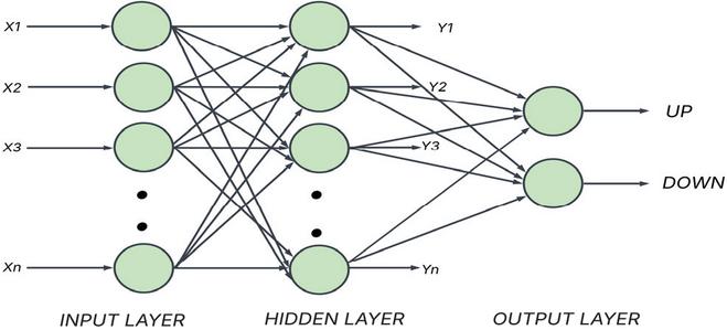
Figure 5 Neural Network Structure.
Multi-Layer Perceptron (MLP) is a feedforward ANN composed of one input layer, one or more hidden layers, and one output layer. Each neuron is fully connected to all the neurons of the previous layer. MLP can also model non-linear relationships well, which conventional linear methods cannot handle [32].
Deep Neural Network (DNN) is an extended version of MLP that has multiple hidden layers. It is used for high-dimensional and complex data where deep feature extraction is required. Each layer learns a feature abstraction level, so the system progressively moves from raw input to high-level decision [33].
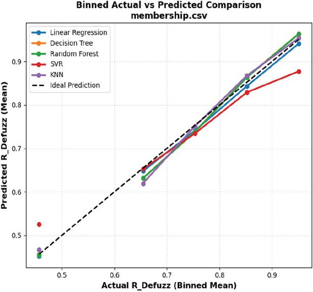
Figure 6 Actual Reliability vs. Predicted Reliability for -cut.
6.2 Performance of Proposed ML Models
ML models are trained to predict system performance metrics (such as failure rate, efficiency, response, etc.) based on the input features. These algorithms can understand hidden patterns within the data and can give accurate predictions even on new/unseen data. The crisp defuzzified & -cut values (Table 3) are used as input features of the ML models. The performance of all ML models are shown in Figures 6 and 7.
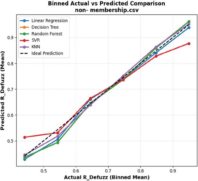
Figure 7 Actual vs. Predicted Reliability for -cut.
For the validation of the obtained results, the actual defuzzified reliability values and the predicted values of the machine learning models are compared. The dashed 45-degree line in the graph represents the ideal prediction. From the analysis of Figures 6 and 7, it is observed that the predicted points of the RF and KNN models are very close to the ideal line, which confirms their high accuracy and strong validation performance. LR and DT also follow an increasing trend, but a slight deviation is observed in some bins. Although a comparatively smaller deviation in SVR is observed in the lower reliability region, the overall positive correlation is maintained. This consistent alignment and monotonic increasing trend validates that the machine learning models have effectively learned the patterns of the defuzzified reliability data. These results confirm that the proposed fuzzy-based reliability assessment framework is statistically sound, accurate, and robust, and its effectiveness is successfully verified by ML-based models.
7 Machine Learning Model Configuration and Hyper Parameters
This section reports the complete configuration of every machine learning model employed in this study, including all hyper parameter values, the validation protocol, and the computational environment, so that all reported results can be independently reproduced. No hyper parameter optimisation was performed at this stage; every model was evaluated using fixed settings, predominantly the library defaults, so that the comparison reflects the intrinsic suitability of each algorithm to the problem rather than the extent of tuning effort applied to it.
7.1 Dataset and Pre-processing
The proposed ML models were trained on the crisp reliability values obtained from the defuzzified -cut and -cut formulations. Because these values are produced by a deterministic analytical expression, the dataset contains no observational noise; the modelling task is therefore one of function approximation rather than statistical estimation.
Table 4 Dataset characteristics and pre-processing settings
| Item | Specification |
| Total samples | 2211 (201 time points 11 -levels) |
| Predictors | Time ; membership level |
| Response variable | Crisp reliability R(t, ) |
| Response range | 0.001536 to 1.000000 |
| Train-test split | 70%/30% (1547/664 samples) |
| Split random seed | 42 |
| Missing-value handling | SimpleImputer (mean strategy) |
| Feature scaling | StandardScaler, applied within pipelines for all distance- and gradient-based learners |
Table 5 Variation of crisp reliability across membership levels
| Time t | Range Across | Relative Spread |
| 1 | 0.998435 0.998573 | 0.014% |
| 10 | 0.696145 0.704487 | 1.191% |
| 50 | 0.098537 0.101884 | 3.342% |
| 100 | 0.017837 0.018595 | 4.172% |
| 200 | 0.001536 0.001610 | 4.697% |
The reliability decays across approximately three orders of magnitude with mission time, whereas the influence of the membership level is comparatively modest. Table 5 quantifies this, reporting the range of the response across all eleven -levels at selected time points.
7.2 Model Hyper parameters
Eight regression algorithms were evaluated: Linear Regression, Ridge Regression, Decision Tree, k-Nearest Neighbours, Support Vector Regression, a single-hidden-layer perceptron (MLP), a three-hidden-layer deep network (DNN), and Random Forest. All hyper parameters were fixed a priori; parameters not listed were retained at their scikit-learn defaults.
Table 6 Hyper parameter values for all models
| Model | Hyperparameter | Value | Description |
| Linear Regression | fit_intercept | True | Library default |
| Preprocessing | Imputer StandardScaler | Pipeline | |
| Ridge Regression | alpha | 1.0 | L2 regularisation strength (default) |
| solver | auto | Library default | |
| Preprocessing | Imputer StandardScaler | Pipeline | |
| Decision Tree | max_depth | None (fully grown) | Library default |
| min_samples_split | 2 | Library default | |
| min_samples_leaf | 1 | Library default | |
| criterion | squared_error | Library default | |
| random_state | 42 | Reproducibility | |
| KNN | n_neighbors | 5 | Library default |
| weights | uniform | Equal neighbour weighting | |
| metric / p | minkowski / 2 (Euclidean) | Library default | |
| Preprocessing | Imputer StandardScaler | Required for distance metric | |
| SVR | kernel | rbf | Radial basis function |
| C | 1.0 | Regularisation parameter (default) | |
| gamma | scale | Kernel coefficient (default) | |
| epsilon | 0.1 | Width of insensitive tube (default) | |
| Preprocessing | Imputer StandardScaler | Required for kernel methods | |
| MLP | hidden_layer_sizes | (64) | Single hidden layer |
| activation | relu | Rectified linear unit | |
| solver | adam | Stochastic optimiser | |
| alpha | L2 penalty | ||
| learning_rate_init | Initial learning rate | ||
| max_iter | 2000 | Maximum epochs | |
| random_state | 42 | Weight initialisation seed | |
| DNN | hidden_layer_sizes | (128, 64, 32) | Three hidden layers |
| activation | relu | Rectified linear unit | |
| solver | adam | Stochastic optimiser | |
| alpha | L2 penalty | ||
| learning_rate_init | Initial learning rate | ||
| batch_size | 64 | Mini-batch size | |
| max_iter | 3000 | Maximum epochs | |
| random_state | 42 | Weight initialisation seed | |
| Random Forest | n_estimators | 100 | Library default |
| max_depth | None (fully grown) | Library default | |
| min_samples_split | 2 | Library default | |
| min_samples_leaf | 1 | Library default | |
| max_features | 1.0 | All features per split | |
| bootstrap | True | Library default | |
| random_state | 42 | Reproducibility |
7.3 ML Model for Table Generation
For the generation of reliability tables, a Random Forest was refitted on the complete design grid with bootstrap resampling disabled. Since the training data are noise-free evaluations of a deterministic function, bagging introduces variance without any compensating bias reduction; disabling it allows every tree to access the complete grid and yields exact reproduction of the tabulated values.
Table 7 ML model configuration
| Setting | Value |
| Estimator | Random Forest |
| Predictors | Time, Alpha (untransformed) |
| n_estimators | 300 |
| max_depth | None (fully grown trees) |
| min_samples_leaf | 1 |
| max_features | 1.0 |
| bootstrap | False |
| criterion | squared_error |
| random_state | 42 |
| Training set | Complete design grid (2211 samples) |
7.4 Validation Protocol
Two complementary evaluation protocols were applied. The first is a conventional random 70/30 hold-out. Because the design grid is dense, however, almost every randomly held-out point lies between two retained neighbours, so this protocol measures local interpolation rather than genuine generalisation.
The second is a structured hold-out in which forty complete time points (every fifth value of t) were removed from training and used exclusively for evaluation. This provides a stricter assessment of the ML model ability to predict at unobserved mission times, and is the protocol on which the generalisation performance reported in this paper is based.
Table 8 Validation results for the ML model
| Protocol | Result |
| Random hold-out (70/30) | ; RMSE |
| Structured hold-out (40 unseen t) | ; mean relative error ; maximum 5.771% |
| Table reconstruction | ; maximum absolute error ; mean relative error 0.0033% |
Table 9 Software environment
| Component | Version |
| Language | Python 3.11 |
| Primary library | scikit-learn 1.8.0 |
| Neural network implementation | sklearn.neural_network.MLPRegressor |
| Supporting libraries | NumPy, pandas, Matplotlib, Seaborn, joblib |
| Global random seed | 42 (all stochastic components) |
7.5 Computational Environment
The ML model is valid only within the fitted domain and . Tree-based ensembles cannot extrapolate beyond the range of the training data and return a constant value outside it; predictions for longer mission times would require either an extended training grid or a parametric extrapolation model.
8 Statistical Result of ML Models
The results obtained from the proposed mathematical model are used to generate the crisp reliability values, which serve as the reference dataset for the machine learning analysis. These crisp reliability values, obtained through the defuzzification of the -cut and -cut formulations, are used as the target reliability data for training and evaluating the ML models. The complete dataset of the crisp reliability values used in this study is provided at the following link: [Data Link]. The goal of applying ML is to determine the prediction accuracy and performance of various learning models in reproducing the system reliability behaviour. The ML models are used to analyse the reliability behaviour of the system in a data-driven way by learning the relationship between the input parameters of the system and the reliability response. The performance of the models is measured using the score, which enables the ML models to be quantitatively compared and the best-performing model to be determined. In the present study, therefore, ML is used mainly for accuracy assessment, performance comparison, and predictive modelling, and not as a substitute for the proposed mathematical reliability model.
Table 10 reports comparative performance on the held-out test partition, ordered by maximum absolute error. Multiple metrics are given because the coefficient of determination alone does not discriminate adequately among the better-performing models.
Table 10 Model performance on the test partition
| Model | R2 (%) | MSE | RMSE | MAE | Max Abs Error |
| Decision Tree | 99.9995 | ||||
| Random Forest | 99.9994 | ||||
| DNN | 99.8244 | ||||
| KNN | 99.7026 | ||||
| MLP | 90.6820 | ||||
| SVR | 88.3368 | ||||
| Ridge Regression | 47.6613 | ||||
| Linear Regression | 47.6556 |
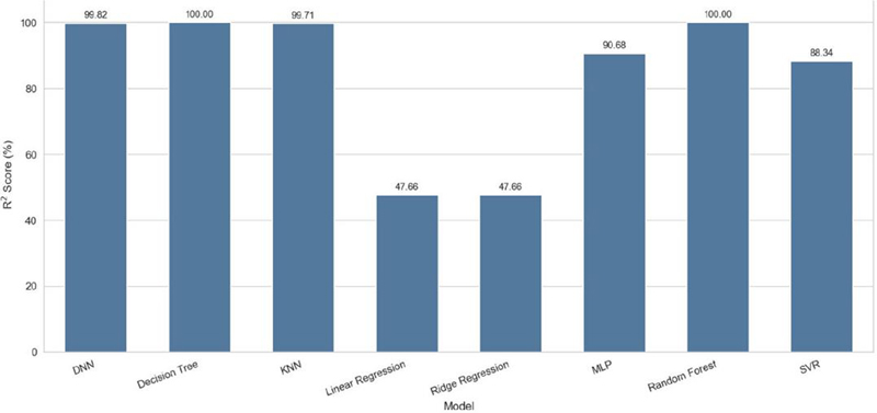
Figure 8 ML Model Performance.
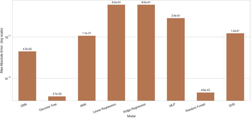
Figure 9 Maximum Absolute Error by all Model.
Three observations follow from these results. First, the tree-based methods separate from the remainder by one to two orders of magnitude in error, since a piecewise-constant approximation is well matched to a dense deterministic grid. Second, the linear models attain only approximately 48%, which is expected: the response decays exponentially and cannot be represented by a linear function of the untransformed predictors. Third, Ridge Regression offers no advantage over ordinary Linear Regression here, because L2 regularisation reduces variance at the cost of bias, and the training data contain no noise for that trade to act upon.
Form the critical study of Table 10, one can acquire that DT and RF consistently achieved the highest score (100%) and very low prediction erros them the most accurate and reliable model for the complex system. Whereas KNN and LR are also strong performers with around 99%, indicating that the data follows linear as well as neighbourhood-based patterns. While DNN give around 98% accuracy, SVR and MLP lagged a bit but still maintained an score close to 90%.
9 Conclusion
In this study, a hybrid approach to analyse the reliability of complex systems by FTA with Triangular IFS, under the consideration of Weibull distribution to express uncertainty in system failure is developed. Multiple supervised ML models such as LR, DT, RF, SVR, KNN, MLP and DNN are used in this study for system performance assessment. From the vital study of obtained results in Sections 5, 6, 7, and 8 it is observed that all the regression models performed quite well, but Decision Tree and Random Forest gives the most accurate and reliable output. Even simple models like Linear Regression and KNN give high accuracy due to structured and consistent data pattern, whereas neural networks (MLP and DNN) also give strong predictions but consumed more time and resources in training. If simplicity and fast training are prioritized, Decision Tree can be considered a suitable choice, whereas Random Forest may be preferred when robustness and generalization are prioritized. Overall, both Decision Tree and Random Forest demonstrated the best predictive performance among the evaluated model.
Overall, the study concludes that a combination of fuzzy reliability modelling and suitable ML model selection can achieve reliable and interpretable predictions for complex engineering systems. In future, authors will try to study optimization-based feature selection, and validation with real industrial data. Also, its practical use as a decision-support tool and cost-reliability trade-offs could be further improved. The results are beneficial for the engineers to effectively handle uncertain failure in complex systems.
References
[1] Suresh, P. V., Babar, A. K., and Raj, V. V. (1996). Uncertainty in fault tree analysis: A fuzzy approach. Fuzzy Sets and Systems, 83(2), 135–141.
[2] Wang, W., Loman, J., and Vassiliou, P. (2004, January). Reliability importance of components in a complex system. In Annual Symposium Reliability and Maintainability, 2004-RAMS (pp. 6–11). IEEE. USA.
[3] Soleimani, M., Pourgol-Mohammad, M., Rostami, A., and Ghanbari, A. (2014). Design for reliability of complex system: Case study of horizontal drilling equipment with limited failure data. Journal of Quality and Reliability Engineering, 2014(1), 524742.
[4] Mi, J., Li, Y. F., Yang, Y. J., Peng, W., and Huang, H. Z. (2016). Reliability assessment of complex electromechanical systems under epistemic uncertainty. Reliability Engineering & System Safety, 152, 1–15.
[5] Torres-Toledano, J. G., and Sucar, L. E. (1998). Bayesian networks for reliability analysis of complex systems. In Progress in Artificial Intelligence – IBERAMIA 98: 6th Ibero-American Conference on AI Lisbon, Portugal, October 5–9, 1998 Proceedings 6 (pp. 195–206). Springer Berlin Heidelberg.
[6] Dhillon, B. S., and Rayapati, S. N. (1986). A complex system reliability evaluation method. Reliability Engineering, 16(2), 163–177.
[7] Juang, Y. S., Lin, S. S., and Kao, H. P. (2008). A knowledge management system for series-parallel availability optimization and design. Expert Systems with Applications, 34(1), 181–193.
[8] Tyagi, V., Arora, R., Ram, M., and Triantafyllou, I. S. (2021). Copula based measures of repairable parallel system with fault coverage. International Journal of Mathematical, Engineering and Management Sciences, 6(1), 322.
[9] Shivani, S., Ram, M., Goyal, N., and Kumar, A. (2023). Analysis of series–parallel system’s sensitivity in context of components failures. RAIRO-Operations Research, 57(4), 2131–2149.
[10] Tekiner-Mogulkoc, H., and Coit, D. W. (2011). System reliability optimization considering uncertainty: Minimization of the coefficient of variation for series-parallel systems. IEEE Transactions on Reliability, 60(3), 667–674.
[11] Hryniewicz, O. (2006). An evaluation of the reliability of complex systems using shadowed sets and fuzzy lifetime data. International Journal of Automation and Computing, 3, 145–150.
[12] Poonia, P. K., Azeez, C., and Rasappan, S. (2026). ANN- Assisted Reliability and Availability of a Warm Standby Repairable Computer Network System. International Journal of Mathematical, Engineering and Management Sciences, 11(2), 1050–1073. https://doi.org/10.33889/IJMEMS.2026.11.2.043.
[13] Wu, J., Yan, S., and Xie, L. (2011). Reliability analysis method of a solar array by using fault tree analysis and fuzzy reasoning Petri net. Acta Astronautica, 69(11–12), 960–968.
[14] Kaushik, M., and Kumar, M. (2022). An application of fault tree analysis for computing the bounds on system failure probability through qualitative data in intuitionistic fuzzy environment. Quality and Reliability Engineering International, 38(5), 2420–2444.
[15] Kaushik, M., and Kumar, M. (2023). Distance and similarity-based aggregation method in intuitionistic fuzzy fault tree analysis. Available at SSRN 4363462.
[16] Bai, H. (2023). Research on network equipment fault detection based on fault tree analysis. Procedia Computer Science, 228, 271–280.
[17] Zacchaeus, M., Ugbebor, J. N., Agbagwa, I. O., and Orikpete, O. F. (2023). Enhancing Safety in Nigeria’s Oil and Gas Sector: A Fault Tree Analysis Approach. The Journal of Engineering and Exact Sciences, 9(11), 18261–18261.
[18] Cao, D., and Bai, G. C. (2020). DNN-based surrogate modeling-based feasible performance reliability design methodology for aircraft engine. IEEE Access, 8, 229201–229218.
[19] Hasan, R., Palaniappan, S., Raziff, A. R. A., Mahmood, S., and Sarker, K. U. (2018, August). Student academic performance prediction by using decision tree algorithm. In 2018 4th International Conference on Computer and Information Sciences (ICCOINS) (pp. 1–5). IEEE.
[20] Olaniyi, A. S., Kayode, S. Y., Abiola, H. M., Tosin, S. I. T., and Babatunde, A. N. (2017). Student’s performance analysis using decision tree algorithms. Annals. Computer Science Series, 15(1), 55–62.
[21] Joseph, P. J., Vaswani, K., and Thazhuthaveetil, M. J. (2006, February). Construction and use of linear regression models for processor performance analysis. In The Twelfth International Symposium on High-Performance Computer Architecture, 2006. (pp. 99–108). IEEE.
[22] Ciulla, G., and D’Amico, A. (2019). Building energy performance forecasting: A multiple linear regression approach. Applied Energy, 253, 113500.
[23] Al-Shehri, H., Al-Qarni, A., Al-Saati, L., Batoaq, A., Badukhen, H., Alrashed, S., …, and Olatunji, S. O. (2017, April). Student performance prediction using support vector machine and k-nearest neighbor. In 2017 IEEE 30th Canadian Conference on Electrical and Computer Engineering (CCECE) (pp. 1–4). IEEE.
[24] Dewi, C., and Chen, R. C. (2019). Random forest and support vector machine on features selection for regression analysis. Int. J. Innov. Comput. Inf. Control, 15(6), 2027–2037.
[25] Bansal, M., Goyal, A., and Choudhary, A. (2022). A comparative analysis of K-nearest neighbor, genetic, support vector machine, decision tree, and long short-term memory algorithms in machine learning. Decision Analytics Journal, 3, 100071.
[26] Wang, J. Q., Nie, R., Zhang, H. Y., and Chen, X. H. (2013). New operators on triangular intuitionistic fuzzy numbers and their applications in system fault analysis. Information Sciences, 251, 79–95.
[27] Kharola, S., Kumar, A., Goyal, N., and Ram, M. (2022, October). Fuzzy reliability modeling of a smart waste bin using triangular intuitionistic fuzzy set. In 2022 10th International Conference on Reliability, Infocom Technologies and Optimization (Trends and Future Directions) (ICRITO) (pp. 1–4). IEEE.
[28] James, G., Witten, D., Hastie, T., Tibshirani, R., and Taylor, J. (2023). Linear regression. In An Introduction to Statistical Learning: With Applications in Python (pp. 69–134). Cham: Springer International Publishing.
[29] Myles, A. J., Feudale, R. N., Liu, Y., Woody, N. A., and Brown, S. D. (2004). An introduction to decision tree modeling. Journal of Chemometrics: A Journal of the Chemometrics Society, 18(6), 275–285.
[30] Boateng, E. Y., Otoo, J., and Abaye, D. A. (2020). Basic tenets of classification algorithms K-nearest-neighbor, support vector machine, random forest and neural network: A review. Journal of Data Analysis and Information Processing, 8(4), 341–357.
[31] Pham, D. T., and Pham, P. T. N. (1999). Artificial intelligence in engineering. International Journal of Machine Tools and Manufacture, 39(6), 937–949.
[32] Singh, J., and Banerjee, R. (2019, March). A study on single and multi-layer perceptron neural network. In 2019 3rd International Conference on Computing Methodologies and Communication (ICCMC) (pp. 35–40). IEEE.
[33] El Fouki, M., Aknin, N., and El Kadiri, K. (2019). Multidimensional Approach Based on Deep Learning to Improve the Prediction Performance of DNN Models. International Journal of Emerging Technologies in Learning, 14(2).
[34] Samal, U., and Raj, M. (2025, March). Integrating fault removal efficiency and S-shaped fault detection in software reliability growth modeling. In 2025 IEEE International Conference on Interdisciplinary Approaches in Technology and Management for Social Innovation (IATMSI) (Vol. 3, pp. 1–5). IEEE.
[35] Samal, U., and Kumar, A. (2025). The impact of learning, fatigue, and dependent faults on software reliability. International Journal of Reliability, Quality and Safety Engineering, 32(02), 2440005.
[36] Samal, U., and Shukla, S. (2025, September). Stacked ensemble with recurrent neural networks for software fault forecasting. In 2025 7th International Conference on Information Systems and Computer Networks (ISCON) (pp. 1–5). IEEE.
Biographies

Deepanshi is a currently pursuing a Ph.D. in Mathematics from Graphic Era Deemed to University, Dehradun, India. With a solid academic foundation, Deepanshi holds a BSc. & MSc. in Mathematics from Mahatma Jyotiba Phule Rohilkhand University, Bareilly.

Akansha Gupta is a distinguished academician in the Department of Computer Science & Engineering at Graphic Era Deemed to be University, Dehradun, Uttarakhand. She possesses more than 20 years of extensive teaching and research experience in the field of Computer Science and Engineering. Her scholarly contributions have been published in several reputed international journals. She has also been granted six Indian patents in recognition of her innovative research work. Her academic interests include Artificial Intelligence, Machine Learning, and advanced computing technologies.

Nupur Goyal is an Associate Professor in the Department of Mathematics at Graphic Era Deemed to be University, Dehradun, India. She earned her B.Sc. in Computer Science (2009, KU Kurukshetra), M.Sc. in Mathematics (2011, H.N.B. Garhwal University), and Ph.D. (2016, Graphic Era University). With 15 years of teaching and 14 years of research experience, her interests lie in reliability theory and operations research. She has published over 90 research papers, book chapters, and edited two books. Dr. Goyal serves as reviewer and guest editor for international journals, is Associate Editor of IJMEMS, and has contributed to organizing numerous conferences, seminars, and workshops.
Journal of Reliability and Statistical Studies, Vol. 20, Issue 1 (2027), 1–36
doi: 10.13052/jrss0974-8024.2011
© 2026 River Publishers