RealTE: Real-time Trajectory Estimation Over Large-Scale Road Networks

Qibin Zhou¹, Qingang Su^2,* and Dingyu Yang³

¹School of International Education, Shanghai Jian Qiao University, Shanghai, China

²School of Kaiserslautern Intelligent Manufacturing, Shanghai Dian Ji University, Shanghai, China

³Alibaba Group, Shanghai, China; School of Electronics and Information, Shanghai Dian Ji University, Shanghai, China

E-mail: zqbin@gench.edu.cn; suqg@sdju.edu.cn; dingyu.ydy@alibaba-inc.com; yangdy@sdju.edu.cn

$^{*}$ Corresponding Author

Received 31 August 2021; Accepted 21 September 2021; Publication 03 January 2022

Abstract

Real-time traffic estimation focuses on predicting the travel time of one travel path, which is capable of helping drivers selecting an appropriate or favor path. Statistical analysis or neural network approaches have been explored to predict the travel time on a massive volume of traffic data. These methods need to be updated when the traffic varies frequently, which incurs tremendous overhead. We build a system $R e a l T E$ , implemented on a popular and open source streaming system $S t o r m$ to quickly deal with high speed trajectory data. In $R e a l T E$ , we propose a locality-sensitive partition and deployment algorithm for a large road network. A histogram estimation approach is adopted to predict the traffic. This approach is general and able to be incremental updated in parallel. Extensive experiments are conducted on six real road networks and the results illustrate RealTE achieves higher throughput and lower prediction error than existing methods. The runtime of a traffic estimation is less than $1$ seconds over a large road network and it takes only $619$ microseconds for model updates.

Keywords: Trajectory prediction, road network partition, histogram estimation.

1 Introduction

Real-time traffic estimation focuses on predicting the travel time of one travel path immediately, which is capable of helping drivers selecting an appropriate or favor path. Transportation managers can control the traffic flow to reduce the congestion when a traffic jam happens. Vehicles could avoid passing some busy roads or rush hours in advance [1]. As a result, it is significant for drivers and transportation managers to forecast the traffic condition in real-time.

In the last decades, with the development of global positioning systems, mobile computing and sensor networking techniques, a massive volume of traffic data has been released from transportation devices and automobiles. It is possible to systematically track and predict the traffic condition. One problem is that, how to efficiently analysis the huge trajectory data, and then accurately estimate the traffic condition immediately [1, 2, 4, 16, 17, 24, 32].

Numerous methods have been applied for traffic prediction. For example, traditional time series methods, autoregressive (AR), autoregressive integrated moving average (ARIMA) [3], machine learning method such as MM-GMRF model [6], and neural network model [7] techniques are explored to estimate the condition. AR or ARIMA are utilized as standard approaches to predict the future values in finance and bank field, but they cannot forecast unexpected variations at rush hours or when some accidents happen. MM-GMRF model [6, 8] presents learning-based algorithms to represent the distributions of traffic conditions on a large road network, but it ignores the specific features of each road, such as idle or busy.

In fact, the traffic condition varies regularly. If the distribution of a road segment has been changed, for example, road congestion, the learning model needs to be modified quickly. The drivers through the busy road segment have to be informed instantly. However, existing transportation systems are unable to support traffic condition forecasting in real-time. The cost of training a deep learning model is very high and the process needs more than several hours or few days, which is not suitable for real-time prediction. For this purpose, this work is designed to deal with three major challenges on real-time traffic prediction:

(1) Updating the training model instantly. Current approaches adopt linear or neural network models to forecast the following numbers. Once new data is collected, the models have to be re-trained. If this training process takes many hours or days, it is not strong enough to support real-time prediction.

(2) A general learning model. As every road has an independent travel time distribution, for example, a prediction model of one busy road cannot directly be applied for an idle road. Some complex models might be suitable for some traffic estimation, but not general for the whole road networks.

(3) The scalability of the whole system. Once new trajectory data have been collected from multiple road segments, it will trigger model updates for each road. The performance and scalability of the processing system will be impacted by high frequency updates, large road segments and limited resources.

In this paper, we revisited our previous work $H i t e$ [13] and extended it in several aspects. The platform of distributed stream system is $S t o r m$ [10] instead of $S 4$ [22]. The new system named RealTE has higher throughput and lower overhead for model updates. A new locality-sensitive algorithm is proposed to partition a large road network into multiple sub-partitions. Moreover, the whole experiments have been redesigned with more datasets, new performance metrics, and more existing methods.

Overall, the main contributions of our work can be listed as below:

1. This paper develops a processing system $R e a l T E$ to predict the travel time on a massive volume of real traffic data. A locality-sensitive partition and deployment algorithm is proposed to process a large road network in parallel to reduce the communication cost and balance the computation cost.

2. We adopt a histogram estimation approach to forecast the traffic. This approach is general for complex traffic prediction and able to be incremental updated in parallel. Since each partition of a large road network are independent, the estimation and road update can be executed concurrently to improve the scalability. Furthermore, this work provides a $H i s t o g r a m U p d a t e$ technique to in a low overhead as soon as fresh data is obtained.

3. Extensive experiments are conducted on six real road networks and the results illustrate RealTE performs higher throughput and lower prediction error than existing methods. The runtime of a traffic estimation is less than $1$ seconds on a large road network and it takes $619$ microseconds for model updates.

The main content of the work is arranged as follows. It firstly presents the problem definition in Section 2. System framework is depicted in Section 3. We report the estimation approach in Section 4, which includes graph partition, histogram-based algorithm, traffic update, and traffic query. Experiments have been conducted in Section 5. Literature review is reported in Section 6. We give a conclusion in Section 7.

2 Problem Definitions

We define terminology for our ensuing discussion and formally present the traffic estimation problem over road networks.

Definition 1 Road Network $G$ .

A road network is a directed, edge-weighted graph and can be defined as $G \to (V_{m}, E_{n}, W e i g h t)$ . $V_{m}$ denotes that the number of vertices is $m$ , and $n$ is the number of edges or roads. Each vertex in a road network is a road junction, and is shared with some connected road segments. Every road (or edge) has a start and end vertices with some weights, which can be denoted as $e = (v_{i}, v_{j}, w_{e})$ . The weight $w_{e}$ is the travel time.

A vehicle with some sensor devices continuously collects the direction and location information, for example, the speed, latitude, longitude and direction of the vehicle, and transmits to a processing or database server.

Definition 2 Trajectory Path $P$ .

A Trajectory path $P$ is defined as a numerical sequence with several time-ordered places, $P = {p_{1}, p_{2}, \dots}$ , and each place $p$ includes ${timestamp, longitude, latitude, speed, direction}$ .

In different hours, the amount of duration required to pass a certain road in $G$ is different, which is an important factor for self-driving. We can define it as travel time.

Definition 3 Travel Time $T$ .

A travel time $T$ is the trip time of going through a certain edge at one timepoint.

The travel time of one edge over time is not static and always evolved. From the open dataset [30], the path of each vehicle can be extracted according the location information. At each sample timestamp, we can apply the average travel time of several vehicles as the condition of one edge.

This work focuses on the problem of predicting the traffic condition timely based on the Trajectory data $P$ .

Definition 4 Traffic Time $T^{'}$ Prediction. We define the traffic time $T^{'}$ calculated via one prediction function $F ()$ . The function $F$ combines some dimensions such as the timepoint $t$ , the edge $e$ , and the Trajectory data $P$ . Then the function is able to be computed by $T^{'} = F (t, e, P)$

As more vehicles consecutively gather their trajectory information to processing nodes, then the system quickly process the data and update the condition as soon as possible. If the execution time is very long, the estimation values will be obsolete.

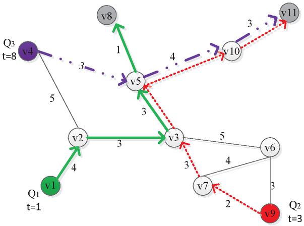
Figure 1 An example road network with three routes.

Figure 1 is an example to show this case. We have three cars and three travel paths( $Q_{1}, Q_{2}, Q_{3}$ respectively). The blue router is from $Q_{1}$ to $v_{8}$ , the red one is from $Q_{2}$ to $V_{11}$ , and the brown one is also traveling from $Q_{3}$ to $V_{11}$ . There exist common sub-paths from these three travel paths. At timepoint $t = 8$ , both $Q_{1}$ and $Q_{2}$ plans to pass the road $v_{3} \to v_{5}$ . At timepoint $t = 11$ , $Q_{2}$ and $Q_{3}$ will enter road $v 5 \to v_{10}$ and $v_{10} \to v_{11}$ . The travel time of $v_{3} \to v_{5}$ will be affected if several vehicles passing this road at timepoint $t = 8$ , and it has to be re-computed to replace the obsolete value $t r a v e l t i m e = 3$ .

One simple update method trains the model again whenever new data is received. It is simple to be implemented and can consider not only the history data, but also the real-time data. To forecast the travel time, the estimation model has to be incremental updated with more real-time traffic.

Definition 5 Real-time Traffic Time Prediction $T^{'}$

Assuming that one new trajectory data $P_{n e w}$ is received, the function $F ()$ needs to be re-computed from $P_{n e w}$ . Given an edge $e$ , we can make the prediction as: $T^{'} = F (t, e, P^{'})$ , in which the $P^{'}$ equals to $P_{o l d} + P_{n e w}$ .

Let’s take an example for real-time prediction. At timestamp $t_{0}$ , our system receives some trajectory data $P_{t_{0}}$ , the model $F ()$ is trained based on the data $P_{t_{0}}$ at $t_{0}$ . The traffic time of the edge $e$ can be estimated by $F (t_{0}, e, P_{t_{0}})$ . After a period of time, i.e., $t_{1}$ , some new trajectory data $P_{t_{1}}$ are collected at the duration $t_{0} t_{1}$ . The model $F ()$ is deprecated and needs to be updated. The real-time prediction will be calculated by new model $F (t_{1}, e, P_{t_{0} + t_{1}})$ . The model at $t_{1}$ could be updated based on the model at $t_{0}$ or re-trained by the trajectory data $P_{t_{0} + t_{1}}$ .

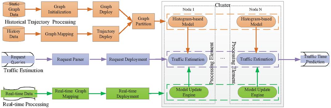
Figure 2 Architecture of $R e a l T E$ .

3 An Overview of Our System

To efficiently support time-dependent traffic estimation and querying in real-time, this paper proposes a distributed architecture, defined as $R e a l T E$ . The details of our system is presented in Figure 2, which contains three major components:

▷ Historical Trajectory Processing Our system firstly partitions a large graph into multiple sub-graphs and deploys them on multiple nodes in a cluster. Meanwhile, the trajectory data are mapped to corresponding graph edges and deployed to some partitions. We design a general algorithm based on histogram to estimate the future travel condition on each edge.

▷ Real-time Traffic Estimation Once a new request is received, an estimation task is generated instantly and sent to the process engine. Request Parser analyzes the task, and gets some parameters of $R e a l T E$ . Then in this module, we can know how many partitions for this road network and how many nodes in this cluster. Some request parameters (such as the source, or the target) are also returned from this parser, which are used for traffic estimation and model update. Request Deployment dispatches the task to the corresponding partition through a $l o c a l i t y$ method. Traffic Estimation in specific partition analyzes the request task (e.g., the edge, timestamp) and predicts the traffic condition. Recall that in Section Problem Definition, the algorithm is processed in an asynchronous mode to support real-time prediction. The results can immediately be served for other applications (e.g., path planning).

▷ Real-time Traffic Update In order to support traffic prediction just in time, the model needs to be updated for each road segment. For a given trajectory data, Real-time Graph Mapping parses the original data into an identifiable format, aiming to mapping it to a processing partition in Real-time Deployment. Once the partition receives the real-time data, Model Update Engine will be triggered to update the model incrementally. The whole process can be executed in parallel to improve the efficiency and scalability.

4 Distributed Traffic Estimation

The original trajectory includes the vehicle’s location information, such as one timestamp and position, that cannot be immediately mapped to the road segment. These data cannot be directly applied for traffic scheduling or navigation. For example, one vehicle has a speed with $30$ kilometers, which denotes normal traffic in a living area, while in an arterial road, this speed might represent to be congestion. Meanwhile, different time regions also have different travel time distributions due to various influencing factors, for example, time of day and day of week. Considering the special features of each road, the estimation model should be adaptive for all road segments, meanwhile, each road segment has its own prediction model.

4.1 Locality-Sensitive Partition and Deployment

Our system starts with partitioning a road network (structured as graph) $G$ into multiple subgraphs such that each subgraph has fewer vertices. The value of partition number $N$ is hard to decide when the graph is larger. In our experiment, we have estimated the parameter $N$ to achieve a suitable number. Two more partitions might share some vertices, which are boundary vertices.

The random partition is simple, and is randomly partitioning some fixed number of vertices into subgraphs. It is the default method in existing big data processing platforms (e.g., Spark [25] or Storm [10]). While the metis-balanced algorithm [9] is a clustering method which considers the density of the graph. For example, some dense area might have fewer vertices while some sparse regions have more vertices. In this paper, we adopt the metis-balanced algorithm to balance the computation cost of each partition.

After the graph partition, we need to allocate the partitions to the cluster nodes. The traditional approach adopts a $H a s h$ function and assigns each subgraph to one processing machine in a cluster. However, the performance would be considerably affected because of frequently edge updates. Specifically, some partitions might appear repeatedly in some cases, and there exist some partitions occur irregularly. That is, the “round-robin deploy method” incurs some imbalance computation, causing some problems such as hotspot partition.

In this paper, we present a locality-sensitive algorithm to improve the performance of our system. After analyzing the dataset, we find that when passing through one subgraph, the neighbors of this partition constantly receive request messages from upper partitions. The network overhead will be consumed when the neighbor partitions are deployed in different processing nodes.

Thus, with the purpose of decreasing the network overhead, we deploy the neighbors as near as possible, and relocated them on same nodes instead of $H a s h$ deployment. As a result, when traversing the road network, the proportion of local computation will be largely improved.

4.2 NLT Histogram-Based Estimation

A partition in our system can be regarded as a subgraph. It contains the features of the vertices and edges. It is able to compute the traffic duration passing through each edge on any timestamp.

Let’s give the example again in Figure 1. When $t = 1$ , the car $Q_{1}$ is at edge $v_{1} \to v_{2}$ . The speed of $Q_{1}$ is defined as $s p e e d_{1}$ , then we obtain a sample data with traffic duration on road $v_{1} \to v_{2}$ by $(t = 1, T_{v_{1} \to v_{2}} = l e n g t h (v_{1} \to v_{2}) / s p e e d_{1})$ . Note that, at timepoint $t = 8$ , there exist two cars running on the edge $v_{3} \to v_{5}$ simultaneously. In this case, the traffic condition needs to be considered all the cars. Since each car has one speed, then the computing formula is $(t = 8, C_{v_{3} \to v_{5}} = l e n g t h (v_{3} \to v_{5}) / a v g (s p e e d))$ .

In a real scenario, the traffic condition of each segment might be variable at any time and each of them has its own distribution. Given a time interval, it is inefficient to estimate the travel time for one road segment. For instance, the road network of New York contains $733 K$ road segments, thus the model needs to process $63$ billion traffic data with each second in a whole day. If a car passes a road segment spending half of one minute, in this duration, we would collect 30 values to denote the travel time for this road. It needs great overhead to maintain the estimation model in a high frequency data collection. Thus, an approximate algorithm is needed to estimate the traffic condition in a large scale of road network.

Histogram models are widely used to represent the data distribution. It is concise and easy to understand for data prediction. A lot of works such as estimating the query size, approximate evaluation, and knowledge discovery have been studied [11]. In the histogram model, the dataset is partitioned into several buckets or sub-sets. In each partition, it stores some statistical metrics to summarize the distribution, which is fewer than the original dataset. The metrics contain the partition boundaries, the average values, the number of values, and the variance. We can query the traffic condition by re-calculating the data model to answer the query.

Our model propose the N-Level-Tree(NLT) [14] to build the histogram with defining partitions in a hierarchical style. The $x$ axis in our model $g$ is time dimension $t$ , and the $y$ axis is the travel time $g (t)$ . Given a road segment, the minimal time is $t_{0}$ , while $t_{m a x}$ is the maximum time for all cars at one segment. Then we can compute the $t_{m a x}$ according to the trajectory data. In this way, it removes the invalided numbers and improves the performance of model construction.

For the time dimension $t$ , the range of $t$ is partitioned into $K$ buckets. One bucket can build its own histogram model $N L T$ . The number of buckets $K$ can be calculated by $K = 2^{N - 1}$ , where $N$ is the level.

In order to construct the $N L T$ model, we start to divide the dimension $t$ into several buckets with equal-size sub-ranges. Then each bucket is assigned to a left node. The leaf number can be calculated by the sum up of related buckets. The whole process is a bottom-up style to continuously insert the values to the parent nodes by accumulating the sibling nodes. The build task will be stop when reaching the root node.

That is, in this model, we only store the left node of the tree and the right node can be computed by a difference of the left node and its parent node. Exactly, we can apply a $32$ bits to represent the root node as $L_{0}$ , and the left child node $L_{1}$ could be defined as $k$ bits where $k = 31$ . Subsequently, the node representation decreases the size of bits by 1 along with the increasing level.

The details of $N L T$ could be depicted by the example $4 L T$ [14]. It is combining $32$ bits to represent the tree in Figure 3. The raw data in a partition $S_{k}$ will be separated into several same sized $K$ sub partitions, where $K$ equals to $2^{4 - 1} = 8$ $δ_{i / j}$ is computed as summing up its child nodes in following stage, for instance, $δ_{3 / 4} = δ_{5 / 8} + δ_{6 / 8}$ . The value $L_{i / j}$ is calculated as the approximate value $δ_{i / j}$ . We can find that $L_{i / j}$ also have some bits to reduce the storage space, i.e., $L_{i / 8}$ only needs 4-bits strings, $L_{i / 4}$ only needs 5-bits strings, and $L_{i / 2}$ only needs 6-bits strings. The construction can be listed in the following statements:

$L_{1 / 2}$	$= < \frac{δ_{1 / 2}}{δ_{1 / 1}} * (2^{6} - 1) > .$
$L_{i / 4}$	$= < \frac{δ_{i / 4}}{δ_{j / 2}} * (2^{5} - 1) > . And (i = 1 \land j = 1), (i = 3 \land j = 2)$
$L_{i / 8}$	$= < \frac{δ_{i / 8}}{δ_{j / 4}} * (2^{4} - 1) > . And (i = 1 \land j = 1),$
	$(i = 3 \land j = 2), (i = 5 \land j = 3), (i = 7 \land j = 4) .$

We can calculate the approximate numbers via summing up the partial values:

{\tilde{δ}}_{i / j} = < \frac{L_{i / j}}{2^{h} - 1} * {\tilde{δ}}_{i^{*} / j^{*}} >

Note that $h$ is the size of values $L_{i / j}$ , ${\tilde{δ}}_{i^{*} / j^{*}}$ is the estimated number of $δ_{i / j}$ ’s parent point. In Figure 3, the estimated number of any $δ_{1 / j}$ is displayed in parentheses. For instance,

${\tilde{δ}}_{1 / 1}$	$= δ_{1 / 1} = 100$
${\tilde{δ}}_{1 / 2}$	$= \frac{L_{1 / 2}}{2^{6} - 1} * {\tilde{δ}}_{1 / 1} = 52$
${\tilde{δ}}_{2 / 2}$	$= {\tilde{δ}}_{1 / 1} - {\tilde{δ}}_{1 / 2} = 48$
	$\dots$
${\tilde{δ}}_{5 / 8}$	$= \frac{L_{5 / 8}}{2^{4} - 1} * {\tilde{δ}}_{3 / 4} X = 7$
	$\dots$

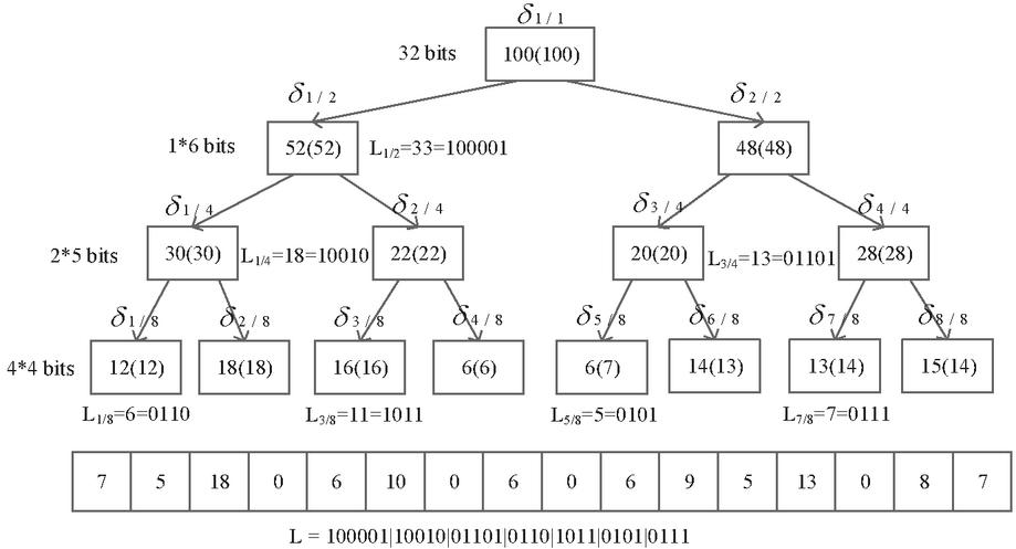
Figure 3 An example of NLT model.

Thus, $4 t h$ level tree contains the whole accumulative number, which are the root number $δ_{1 / 1}$ , and the extra 32-bit number $L$ . Other number could be computed by $δ_{1 / 1}$ and $L$ . It has been verified that $N L T$ performs better than the models, such as Maxdiff [18], V-Optimal [19], and Wavelet [20]. Moreover, the overhead of $N L T$ is lower when constructing the model or answering one query request.

4.3 Estimation Model Update

After building the trajectory estimation model, we can track the travel time based on the timestamp $t_{0}$ . When the system receives new trajectory data, the estimation model has to be updated to accommodate changes. We can define the update into two categories: model structural adjustment and estimation value modification.

The idea of model structural adjustment is shifting left node on the time dimension and building the tree. When the newest time $t_{m a x}$ has been varied, the model will trigger to generate a new bucket to store the values, or it will join in the current newest bucket. Take Figure 4 as an example of model update. When the timepoint $t_{0}$ has passed and the time is up to $t_{1}$ , the model has to be updated by moving left or internal adjustment. We can find that $t_{m a x}$ will be shifted left from $t_{1} - t_{0}$ to $t_{4} \to t_{3}$ . However, since the maximal time has been modified by some vehicle paths, it gets a larger timestamp than $t_{3}$ . In this instance, our system will generate another bucket to store the data distribution in $t_{3} \to t_{4}$ .

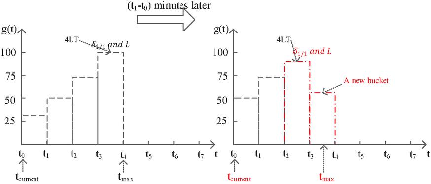
Figure 4 Estimation model update.

Another one is updating the node value in the $N L T$ but not changing the structure of $N L T$ . When the traffic condition has been varied at time $t$ , the travel time on the former $N L T$ model would be expired. The traffic distribution has to be modified to adapt the variation. From previous statement, the summary traffic time $δ_{1 / 1}$ and the value $L$ displayed in Figure 4 are store in the $N L T$ That means we should update two values $δ_{1 / 1}$ and $L$ at same time. After the value $δ_{1 / 1}$ is computed by our algorithm, we can update it straightforwardly through the node index. As the value $L$ denotes the hierarchy of estimation model, it needs some effort to complete the updating.

In order to quickly update the value $L$ , we propose an algorithm using updating local. We first detect the affected branches by the update event. For instance, one node is updated, its parent node is naturally affected. In the same way, the parent’s parent also needs to be checked. If the parent belongs to the left branch, the value $L$ of the parent node will be modified. If not, the value $L$ in the right parent node would not be modified. The processes are presented in the Algorithm 16 The time complexity of model update is $O (l o g M)$ at one timestamp $t$ .

Algorithm 1 Histogram update algorithm

1: One branch $δ_{i / j}$ is updated: $δ_{i / j} = δ_{i / j} + ϵ$

2: $T_{0}, T_{1}, \dots, T_{n}$ , where $T_{0} = δ_{0 / 0}$ , $T_{i}$ is $T_{i + 1}$ ’s parent, $T_{n}$ is the parent of $δ_{i / j}$

3: $L (T_{i})$ is the integer of $T_{i}$ node

4: $k$ is the integer length of $T_{1}$ node

5: $δ_{0 / 0} = δ_{0 / 0} + ϵ$

6: $c = δ_{0 / 0}$

7: for $i \in (1, n)$ do

8: if $T_{i}$ is the left node of $T_{i - 1}$ then

9: $t m p = \frac{L (T_{i})}{2^{k - i + 1} - 1} * (c - ϵ)$

10: $L (T_{i}) = \frac{t m p + ϵ}{c} * (2^{k - i + 1} - 1)$

11: $c = t m p + ϵ$

12: else if $T_{i}$ is the right node of $T_{i - 1}$ then

13: $s b (T_{i})$ is the left brother node of $T_{i}$

14: $t m p = \frac{L (s b (T_{i}))}{2^{k - i + 1} - 1} * (c - ϵ)$

15: $L (T_{i}) = \frac{t m p}{c} * (2^{k - i + 1} - 1)$

16: $c = c - t m p$

4.4 Traffic Estimation

Based on former sections, we can naturally achieve the estimation algorithm on the travel time. The training data are extracted by the trajectory data. The model has been ready and we can input the timestamp and the road index. Then we can get the travel time.

Furthermore, we can query a range between two vertices or two-time duration due to the contribution of the histogram. The histogram model will estimate all $\tilde{σ}$ numbers to deal with the values included in the request $Q$ . We attempt to apply this $\tilde{σ}$ numbers to the top stages of the $N L T$ model, as they own the most accurate values. If need be, the estimation can be executed to predict the futures in a deeper granularity.

Supposing that the request area $Q$ covers the former thirteen points in Figure 3, the computation can be achieved by ${\tilde{σ}}_{1 / 2} + {\tilde{σ}}_{3 / 4} + 0.5 * {\tilde{σ}}_{7 / 8} = 52 + 20 + (0.5) (13) = 78.5$ . Note that, the first two points assess the contributions of summing up the first eight and the next four. While the last point predicts the thirteenth number using the continuous hypothesis. The exact result is $85$ , thus we can calculate the prediction error as $8 %$ . When the request area is larger than one bucket, the prediction is also able be computation in the same way.

5 Experiments

5.1 Experiment Setup and Datasets

Experiment Setup. We have implemented $R e a l T E$ internally in Apache $S t o r m$ [10], which is a popular stream processing system which is easy to develop applications to support real-time data processing. Since each road has continuously vehicles and repeatedly provides events for transportation systems, it is very suitable for us to apply streaming system to process unbounded data.

Note that our previous system $H i t e$ [13] is implemented on Apache $S 4$ , which is an earlier platform for stream processing than $S t o r m$ . The reason to replace the platform is that $S 4$ has been voted to stop maintaining the codes. Moreover, the performance of $S 4$ is lower than $S t o r m$ , which has been optimized and applied to process high speed real-time data in some big data companies, such as Twitter and Alibaba.

Our system $R e a l T E$ is deployed in a 10 nodes cluster. The CPU model is Xeon E5607 Quad Core CPU (2.27GHz) and the memory size is 32GB. The operating system is Ubuntu 14.04. All nodes are connected via Ethernet with a bandwidth of 1Gbps. We pick up one as the master node and others for slave nodes. The master node is responsible for resource management and the scheduling. Although the master node can be shared with a slave node, we still arrange it as an independent node because master node will consume some CPU and memory resources. If one node is allocated as master node and slave node, this node will have less resource for data processing. It might incur some imbalance with other slave nodes.

Datasets. First, we use five real road networks with travel time from US road networks [30]. The information of related road networks in our experiment is listed in Table 1. The sizes of datasets are between 320K and 14 million vertices, and between 800K to 34 billion roads. In the experiment, the default road network is $C A L$ as it is a moderate size dataset to evaluate the efficiency.

Meanwhile, we also assess Beijing’s real dataset, that includes the 10,357 vehicles’ GPS data from February 2 to February 8 [28]. In this dataset, it has 154K vertices and 337K edges of Beijing. Each tuple is a series of GPS data including timepoint and position.

Table 1 Road network datasets

Name	Region	Vertex Number	Edge Number
BAY	San Francisco Bay Area	321,270	800,172
FLA	Florida	1,070,376	2,712,798
CAL	California and Nevada	1,890,815	4,657,742
E	Eastern USA	3,598,623	8,778,114
CTR	Central USA	14,081,816	34,292,496
BJ	Beijing	154,662	337,662

Evaluation methods. In order to evaluate the algorithm, we compare our model $H i s t$ with four baseline methods for real-time traffic estimation.

• Auto-Regressive (AR). It uses a linear combination of past travel time to predict the traffic conditions. It is a basic regression method.

• Exponential Smoothing (ES). This approach adopts a rule to smooth temporal data via an exponential time window model. It is applied to compute the decreasing weights over time. This method is general for time-series data analysis.

• Multi-modal Gaussian Markov Random Field (MM-GMRF). This model captures the interrelationship on the travel time metric, including adjacent edges, and the value of stoppings on the edges. It applies Markov model to calculate the relation between stopping and unstopping for neighboring edges.

• Deep origin-destination (DeepOD). It designs a consolidated deep network method, which is able to completely explore historical trajectory data, road networks. It also combines some other data (such as weather data, and traffic data) to estimate the traffic duration.

Evaluation metrics. Our model $H i s t$ is evaluated with other models based on several popular metrics. Mean relative error (MRE) is the average ratio of the absolute error between a prediction and the real value in Equation (1). Mean absolute error (MAE) is the average difference between between a prediction and the real value in Equation (2). In the Equations, $i$ denotes one edge, $n$ is the total number of edges in a road network, $y_{i}$ is the ground truth of travel time of edge $i$ , ${\hat{y}}_{i}$ is the estimated value of edge $i$ ’s travel time:

$MRE$	$= \frac{\sum_{i} \| {\hat{y}}_{i} - y_{i} \|}{\sum_{i} y_{i}}$	(1)
$MAE$	$= \frac{\sum_{i} \| {\hat{y}}_{i} - y_{i} \|}{n}$	(2)

Specifically, we utilize two other metrics to evaluate the performance of our system: the runtime of the estimation and the throughput of the system. The runtime refers that the latency of the query request. It can be computed by the difference between the received timestamp and the processed timestamp. The throughput is the highest number of queries supported by the system in a time interval (e.g., 1 minute).

Experiment Parameters. In our experiment, we estimate the performance efficiency when changing some parameter values, such as the number of nodes, the number of graph partitions, the frequency of edge updates in one minute, the number of requests in one minute. All the parameters are described in Table 2. The bold one is the default value.

Table 2 Experiment parameters

Cluster nodes	1, 2, 3, 4, 5, 6, 7, 8, 9
Graph partition	10, 100, 500, 1000, 5000, 10000
Update frequency	1000, 5000, 10000, 50000, 100000
Queries	100, 500, 1000, 5000, 10000

5.2 Effectiveness of Graph Partition

In order to evaluate the performance of graph partition, we compare the performance of different partition strategies: $H a s h$ vs Locality-Sensitive ( $L S$ ). $H a s h$ is randomly mapping each sub-graph to one certain physical machine via a $h a s h$ function, while $L S$ utilizes a locality sensitive method and deploys the neighbor partitions to the same machine as possible.

We evaluate the efficiency of the system by changing the number of processing machines. The dataset used in this experiment is $C A L$ , which is a moderate road network. From Figure 5, it is easy to find that $L S$ partition is superior to $H a s h$ partition on runtime and throughput. The main reason is that $L S$ adopts the locality-sensitive partition and deployment, that allocates neighbor partitions together. Then this method can largely reduce the network overhead when querying neighbor traffic condition.

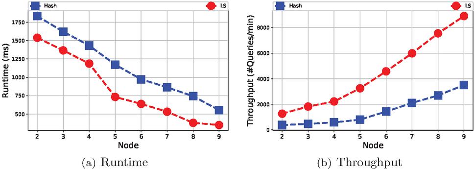
Figure 5 Performance w.r.t. increasing number of nodes.

We also study the performance on $H a s h$ and $L S$ by changing the size of graph partitions. Figure 6 depicts that, in the partition set $S = [10, 100, 500, 1000, 5000, 10000]$ , the optimal number is 1000. That means the number of partitions $n u m_{partition} = 1000$ achieves the minimal runtime and the maximal throughput. If the partition number is very small (such as 10), the performance of both methods is not well. Meanwhile, if the number is very large (such as more than 10000), the efficiency of the system significantly decreases. An appropriate partition number will be conducive to the parallelism ability and reducing the chance of CPU resource contention.

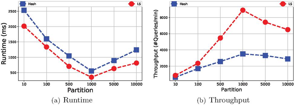
Figure 6 Performance w.r.t. increasing number of partitions.

5.3 Effectiveness of Traffic Estimation

We compare the estimation accuracy with existing algorithms on six datasets. The queries are generated by randomly selecting two vertices in different sub-graphs for each dataset. The default settings are: $n u m_{queries}$ equals to $1000$ , $n u m_{nodes}$ is $9$ , and $n u m_{partitions}$ is $1000$ . The metrics in this experiment are $M A E$ and $M R E$ . Figure 7 illustrates that all methods perform various prediction results on different road networks. We find that none-linear methods outperform than linear methods. The reason is that the travel time is not linearly related. Moreover, we find that when increasing the scale of the road networks, the $M A E$ and $M R E$ metrics of all methods display similar tendency in Figure 7. The larger road network is, the higher prediction error they perform. WE can see that $C T R$ has higher prediction error than road networks $B a y$ and $B J$ . Last but not least, $D e e p O D$ is a deep learning technology, which can approximately fits any function. $D e e p O D$ has close prediction accuracy with our method $H i s t$ . On road networks $C A L$ and $C T R$ , $D e e p O D$ has lower error than $H i s t$ , while $H i s t$ is better on other road networks. In general, our method $H i s t$ performs the better on all metrics than existing methods.

We also compare the performance of traffic estimation on all methods. The setting is similar with Figure 7. The results show that the runtime and throughput on six road networks in Figure 8. Linear methods $A R$ and $E S$ have less estimation time than non-linear methods. Deep learning methods, such $D e e p O D$ need more prediction overhead than other methods. With increasing the size of road network, all methods require more time to complete the prediction and the throughput is decreasing on all road networks. Generally, we can find that $H i s t$ outperforms other methods.

Figure 7 The accuracy evaluation of all methods.

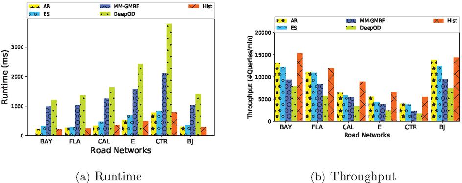
Figure 8 The performance of all methods.

5.4 Performance of Traffic Updates

In order to support real-time traffic estimation, we study the performance of model update once the road network is changed. The update frequency is $10000$ , which means that the system will receive $10000$ edge-updating requests in one minute. The results are shown in Table 3. We can find that the methods $M M - G M R F$ and $D e e p O D$ have a huge latency (more than 1 hour) to complete the updates. The reason is that $M M - G M R F$ and $D e e p O D$ have to run a complex or deep network training process to achieve a stable state, which shows that they are not suitable for real-time update. Moreover, the average runtimes of $A R$ , $E S$ and $H i s t$ are 1157 ms, 1799 ms and 619 ms, respectively. Our method has a lower update runtime than the linear models $A R$ and $E S$ , since we adopt a locality algorithm for edge updates, instead of re-training the model.

Table 3 Performance of traffic updates (ms)

Road Network	AR	ES	MM-GMRF	DeepOD	Hist
BAY	848	1340	$3.7 * 10^{6}$	$5.4 * 10^{6}$	360
FLA	950	1519	X	X	490
CAL	1046	1756	X	X	653
E	1273	1916	X	X	843
CTR	1850	2865	X	X	988
BJ	980	1402	X	X	380

6 Related Work

We summarize some works on data mining for traffic prediction in a vehicular network. Both academic and industrial communities have published several papers and released some products on this area. For example, traditional time series methods, autoregressive (AR), autoregressive integrated moving average (ARIMA) [3], exponential smoothing [5] are popular to predict the traffic condition. Statistical or machine learning approaches [40, 23, 33, 34, 12, 7, 35, 42, 15, 39] are recently adopted to estimate the travel distribution or navigation recommendation.

Historical traffic estimation: Lal et al. [36] adopt an independent server to consistently process the trajectory events through a sensor network. They classify the vehicles into some clusters, and connect the similar class with an ad-hoc network. The clusters can share the data with its neighbors in a low overhead.

The work [33] utilizes network storage for historical location information of vehicles, and gathers vehicle paths through the network between vehicles and sensor devices. Some papers [38, 21, 33] focus on past trajectories with massive tracing data for taxi scheduling.

Real-time traffic estimation: Several researches employ both past and real-time data to estimate the traffic condition. [40] collects sensor data by a probe framework. The model in this work considers the new data of each edge in a vehicle network and predicts the future condition. The authors in [35] combine past and real-time traffic data to forecast the short and long period of travel speed for each vehicle. The proposal in [41] analyzes the original data to infer the position, and to predict the travel duration using a linear model. This model can be executed in a low latency and be suitable for real-time prediction. The work [38] combines real time trajectory data and past data to learn the behavior of drivers according the GPS data. Then they recommend a new and faster path for each driver through a public service.

7 Conclusion

We revisited our previous work $H i t e$ [13] and extended it in several aspects, such as the new implementation platform $S t o r m$ , a locality-sensitive partition and deployment method to improve the parallelism. We also redesigned the experiments with more datasets, new performance metrics, and more existing methods. The new system $R e a l T E$ has been evaluated on six real road networks to predict the travel time on a massive volume of real traffic data. A histogram estimation approach is adopted to predict the traffic. This approach is general and able to be incremental updated in parallel. The results illustrate RealTE achieves higher throughput and lower prediction error than existing methods. The runtime of a traffic estimation is less than $1$ seconds on a large road network and it takes $619$ microseconds for model updates.

Acknowledgements

This work is supported by the National Nature Science Foundation of China under grants No. 61702320 and Shanghai Municipal Education Commission Funds of Young Teacher Training Program No. ZZSDJ17021.

References

[1] Guerrero-Ibáñez, Antonio and Flores-Cortés, Carlos and Damián-Reyes, Pedro and Andrade-Aréchiga, M and Pulido, JRG (2012). Emerging technologies for urban traffic management. Urban Development, 59.

[2] Ma, J., Chan, J., Ristanoski, G., Rajasegarar, S., and Leckie, C. (2019). Bus travel time prediction with real-time traffic information. Transportation Research Part C: Emerging Technologies, 105, 536–549.

[3] Lee, S., and Fambro, D. B. (1999). Application of subset autoregressive integrated moving average model for short-term freeway traffic volume forecasting. Transportation Research Record, 1678(1), 179–188.

[4] Zhang, D., Yang, D., Wang, Y., Tan, K. L., Cao, J., and Shen, H. T. (2017). Distributed shortest path query processing on dynamic road networks. The VLDB Journal, 26(3), 399–419.

[5] Chan, K. Y., Dillon, T. S., Singh, J., and Chang, E. (2011). Neural-network-based models for short-term traffic flow forecasting using a hybrid exponential smoothing and Levenberg–Marquardt algorithm. IEEE Transactions on Intelligent Transportation Systems, 13(2), 644–654.

[6] Hunter, T., Hofleitner, A., Reilly, J., Krichene, W., Thai, J., Kouvelas, A., and Bayen, A. (2013). Arriving on time: estimating travel time distributions on large-scale road networks. arXiv preprint arXiv:1302.6617.

[7] Yuan, H., Li, G., Bao, Z., and Feng, L. (2020). Effective travel time estimation: When historical trajectories over road networks matter. In Proceedings of the 2020 ACM SIGMOD International Conference on Management of Data (pp. 2135–2149).

[8] Box, G. E., Jenkins, G. M., Reinsel, G. C., and Ljung, G. M. (2015). Time series analysis: forecasting and control. John Wiley and Sons.

[9] Karypis, G., and Kumar, V. (1998). A fast and high quality multilevel scheme for partitioning irregular graphs. SIAM Journal on scientific Computing, 20(1), 359–392.

[10] Twitter Storm. https://github.com/nathanmarz/storm

[11] Babcock, B., Babu, S., Datar, M., Motwani, R., and Widom, J. (2002). Models and issues in data stream systems. In Proceedings of the twenty-first ACM SIGMOD-SIGACT-SIGART symposium on Principles of database systems (pp. 1–16).

[12] Hua, Y. A. N. G., and Xing, W. E. I. (2020). An Application of CHNN for FANETs routing optimization. Journal of Web Engineering, 830–844.

[13] Yang, D., Wang, F., and Ji, C. (2016). Hite: Histogram-based traffic estimation on real-time trajectory. In IEEE ICSAI (pp. 444–449). IEEE.

[14] Buccafurri, F., Lax, G., Sacca, D., Pontieri, L., and Rosaci, D. (2008). Enhancing histograms by tree-like bucket indices. The VLDB journal, 17(5), 1041–1061.

[15] Fu, K., Meng, F., Ye, J., and Wang, Z. (2020). Compacteta: A fast inference system for travel time prediction. In Proceedings of the 26th ACM SIGKDD International Conference on Knowledge Discovery and Data Mining (pp. 3337–3345).

[16] Yang, D., Zhang, D., Tan, K.L., Cao, J. and Le Mouël, F., 2014. CANDS: continuous optimal navigation via distributed stream processing. Proceedings of the VLDB Endowment (PVLDB), 8(2), pp.137–148.

[17] Zhang, D., Yang, D., Wang, Y., Tan, K.L., Cao, J. and Shen, H.T., 2017. Distributed shortest path query processing on dynamic road networks. The VLDB Journal, 26(3), pp. 399–419.

[18] Poosala, V., Haas, P. J., Ioannidis, Y. E., and Shekita, E. J. (1996). Improved histograms for selectivity estimation of range predicates. ACM Sigmod Record, 25(2), 294–305.

[19] Jagadish, H. V., Koudas, N., Muthukrishnan, S., Poosala, V., Sevcik, K. C., and Suel, T. (1998). Optimal histograms with quality guarantees. In VLDB (Vol. 98, pp. 24–27).

[20] Matias, Y., Vitter, J. S., and Wang, M. (1998). Wavelet-based histograms for selectivity estimation. In Proceedings of the 1998 ACM SIGMOD international conference on Management of data (pp. 448–459).

[21] Yang, D., Guo, J., Wang, Z. J., Wang, Y., Zhang, J., Hu, L., … and Cao, J. (2018). Fastpm: An approach to pattern matching via distributed stream processing. Information Sciences, 453, 263–280.

[22] Neumeyer, L., Robbins, B., Nair, A., and Kesari, A. (2010, December). S4: Distributed stream computing platform. In 2010 IEEE International Conference on Data Mining Workshops (pp. 170–177). IEEE.

[23] Yang, D., Cao, J., Fu, J., Wang, J. and Guo, J., 2013. A pattern fusion model for multi-step-ahead CPU load prediction. Journal of Systems and Software, 86(5), pp. 1257–1266.

[24] Zhang, D., Ding, M., Yang, D., Liu, Y., Fan, J. and Shen, H.T., 2018. Trajectory simplification: an experimental study and quality analysis. Proceedings of the VLDB Endowment, 11(9), pp. 934–946.

[25] Spark. http://spark.incubator.apache.org

[26] Flink. http://flink.apache.org

[27] Hilger, M., Köhler, E., Möhring, R. H., and Schilling, H. (2009). Fast point-to-point shortest path computations with arc-flags. The Shortest Path Problem: Ninth DIMACS Implementation Challenge, 74, 41–72.

[28] Zheng, Y., Liu, Y., Yuan, J., and Xie, X. (2011). Urban computing with taxicabs. In Proceedings of the 13th international conference on Ubiquitous computing (pp. 89–98).

[29] Wei, H., Wang, Y., Forman, G., Zhu, Y., and Guan, H. (2012). Fast Viterbi map matching with tunable weight functions. In Proceedings of the 20th international conference on advances in geographic information systems (pp. 613–616).

[30] US Road Network. http://www.dis.uniroma1.it/challenge9/download. shtml

[31] Nakata, T., and Takeuchi, J. I. (2004). Mining traffic data from probe-car system for travel time prediction. In Proceedings of the tenth ACM SIGKDD international conference on Knowledge discovery and data mining (pp. 817–822).

[32] Lei, J., Chu, X., and He, W. (2021). Trajectory Data Restoring: A Way of Visual Analysis of Vessel Identity Base on OPTICS. Journal of Web Engineering., 20(2), 413–430.

[33] Merah, A. F., Samarah, S., and Boukerche, A. (2012). Vehicular movement patterns: a prediction-based route discovery technique for VANETs. In 2012 IEEE International conference on communications (ICC) (pp. 5291-5295).

[34] Zhang, B., Xing, K., Cheng, X., Huang, L., and Bie, R. (2012). Traffic clustering and online traffic prediction in vehicle networks: A social influence perspective. In 2012 Proceedings IEEE Infocom (pp. 495–503).

[35] Pan, B., Demiryurek, U., and Shahabi, C. (2012). Utilizing real-world transportation data for accurate traffic prediction. In 2012 IEEE 12th International Conference on Data Mining (pp. 595–604).

[36] Abraham, S., and Lal, P. S. (2012). Spatio-temporal similarity of network-constrained moving object trajectories using sequence alignment of travel locations. Transportation research part C: emerging technologies, 23, 109–123.

[37] Chen, L., Lv, M., and Chen, G. (2010). A system for destination and future route prediction based on trajectory mining. Pervasive and Mobile Computing, 6(6), 657–676.

[38] Yuan, J., Zheng, Y., Xie, X., and Sun, G. (2011). Driving with knowledge from the physical world. In Proceedings of the 17th ACM SIGKDD international conference on Knowledge discovery and data mining (pp. 316–324).

[39] Chen, F., Chen, D., Wang, L., and Botao, Y. (2021). Optimal Design of Electrical Capacitance Tomography Sensor and Improved ART Image Reconstruction Algorithm Based On the Internet of Things. Journal of Web Engineering, 1027–1052.

[40] Nakata, T., and Takeuchi, J. I. (2004). Mining traffic data from probe-car system for travel time prediction. In Proceedings of the tenth ACM SIGKDD international conference on Knowledge discovery and data mining (pp. 817–822).

[41] Lee, W. H., Tseng, S. S., and Tsai, S. H. (2009). A knowledge based real-time travel time prediction system for urban network. Expert systems with Applications, 36(3), 4239–4247.

[42] Xu, H., and Ying, J. (2017). Bus arrival time prediction with real-time and historic data. Cluster Computing, 20(4), 3099–3106.

Biographies

Qibin Zhou, received her M.Sc. degree from Huazhong University of Science and Technology in 2013. She is the deputy director of the Information Office and the vice president of the college of International Education in Shanghai Jianqiao University now. Her present research interests include network security, data analysis, smart campus construction, etc.

Qinggang Su, received the B.Sc. degree in Computer Science from Anhui University of Technology in 2002, and got the M.Sc. degree in Communication Engineering in Shanghai Jiao Tong University, and is studying for Ph.D. degree at East China Normal University. He became a faculty member in the school of electronic information, Shanghai Dianji University China from 2002, and he is the vice dean of Chinesisch-Deutsche Kolleg für Intelligente Produktion of Shanghai Dianji University now. He is a member of China Computer Federation (CCF), and his research is currently focused on wireless networks, 5G application and smart manufacturing.

Dingyu Yang received the B.E. and M.E. degrees from the Kunming University of Science and Technology, and the Ph.D. degree from the Shanghai Jiao Tong University. He is currently a data scientist at Alibaba Group. His research interests include resource prediction, anomaly detection in cloud computing and distributed stream processing.