A Study on Traffic Prediction for the Backbone of Korea’s Research and Science Network Using Machine Learning
Chanjin Park1, 2, Wonhyuk Lee1,*, Moon-Hyun Kim2, Ung-Mo Kim2, Taehong Kim3 and Seunghae Kim1
1Korea Research Environment Network Center, Korea Institute of Science and Technology Information, Daejeon, Korea
2College of Information and Communication Engineering, Sungkyunkwan University, Suwon, Korea
3Dept of Korean Medical Data, Korea Institute of Oriental Medicine, Daejeon, Korea
E-mail: livezone@kisti.re.kr
*Corresponding Author
Received 30 September 2021; Accepted 08 March 2022; Publication 23 July 2022
Abstract
To fix network congestion resulting from the increase in high volume traffic in data-intensive science and the increase in internet traffic due to COVID-19, there has been a necessity of traffic engineering through traffic prediction. For this, there have been various attempts from a statistical method such as ARIMA to machine learning including LSTM and GRU. This study aimed to collect and learn KREOENT backbone and subscribers’ traffic volume through diverse machine learning techniques (e.g., SVR, LSTM, GRU, etc.) and predict maximum traffic on the following day.
Keywords: Traffic prediction, machine learning, SVR, LSTM, GRU, KREONET.
1 Introduction
With the emergence of COVID-19 and various data centers and data-intensive science, Internet traffic volume has rapidly increased these days. The simplest solution is to increase network bandwidth. However, it takes a lot of money to keep increasing network bandwidth. For efficient network management, therefore, it is required to increase bandwidth up to the amount needed for circuits by predicting network traffic volume or avoid such congestion through traffic engineering.
So far, there have been various attempts to predict network traffic. In statistics, auto-regressive moving average(ARMA), auto-regressive integrated moving average (ARIMA) [1, 2] and Holt-Winters algorithm [3] have been commonly used. Recent studies have found that machine learning approaches such as LSTM and GRU are more accurate than ARIMA and Holt-Winters algorithm. In a study by Nandini Krishnaswamy, 24-hour traffic prediction using stacked LSTM improved by more than 70% in average [4].
According to conventional traffic prediction studies, datasets were created by collecting flows and learned, using a machine learning model. However, There are too many flows that occur in a large-capacity network such as an ISP, making it difficult to collect. In the case of KREONET, about 1.4 billion flows/day, 100 GB of flow is collected. Hence, this study attempted to make datasets by collecting traffic volume every 5 minutes. In addition, the maximum value on the following day was predicted instead of forecasting total traffic directly, using machine learning such as SVR, LSTM and GRU. After all, it is difficult to predict such traffic 24 hours. Even successful prediction (90% or higher) means that the traffic was predicted fairly well in average, not that the exact traffic volume was estimated. From a traffic engineer’s perspective, the maximum value on the following day can be most useful. Based on such prediction, bandwidth from the previous day can be adjusted dynamically. Therefore, this study focused on predicting the maximum value.
2 Related Works
In this chapter, diverse network traffic prediction methods such as SVR, LSTM and GRU are reviewed. Furthermore, performance metrics including root mean square error (RMES), mean absolute percentage error (MAPE) score are stated.
2.1 Support Vector Regression (SVR)
SVR is a regression-analysis version of the commonly used support vector machine (SVM). This machine learning method was proposed by Vladmir N. Vapnik, Harris Drucker, Chirs J.C. Buges et al. in 1996 [5]. The -insensitive loss function was applied to the SVM regression model, enabling the prediction of real numbers randomly [5]. First, inputs are mapped to the high-dimensional feature space. Then, a linear function associated with the results is found [6]. SVR uses a linear estimation function as shown in Equation (1) below:
| (1) |
In other words, SVR converts non-linear regression in a low-dimensional input space (x) into linear regression in high-dimensional configuration space (F). (-insensitive loss function) is expressed with cost function used in SVR as shown in Equation (2.1) below:
Weight vector () and constant () in the linear estimation function Equation (1) of SVR can be estimated by the normalized hazard function as shown in Equation (3) below:
| (3) |
is a normalization term coordinating a balance between complexity and accuracy. Here, ‘’ refers to a constant used in balancing empirical risk and normalization term. Both ‘’ and ‘’ are set by a user.
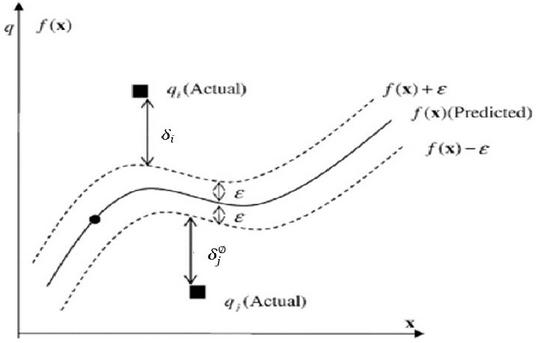
Figure 1 The SVR using e-insensitive loss function [3].
In SVR, margin is maximized by keeping and forecast () within ‘’. Using slack variables, Equation (3) is converted into Equation (2.1):
| Min: | ||
| (4) |
If Lagrange multiplier and Karush-Kuhn-Tucker conditions are applied to Equation (2.1), the SVR regression function can be derived as follows [5]:
| (5) |
In SVR, the inner product is done in a relatively low-dimensional input space by adopting the kernel trick. Then, it is mapped into a high-dimensional space, simplifying calculation. For this, the kernel function () of Equation (5), which refers to the multiplication of the inner product of and , is used.
2.2 Long Short-Term Memory (LSTM)
As a part of RNN, LSTM was proposed to fix long-term dependencies. It was introduced by Hochreiter and Schmidhuber (1997) [7] and has been upgraded since then. It has taken good care of issues from various fields, and it is still commonly used.
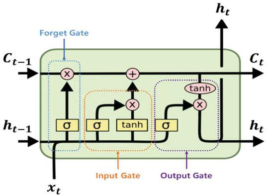
Figure 2 LSTM cell state [8, 9].
The first step is to decide what information would be thrown away from the cell state, and such decision is made by a sigmoid layer. Therefore, this step is called, ‘forget-gate layer’ and can be expressed as Equation (6). In this step, the value between ‘0’ and ‘1’ is sent to ‘’ after getting and . If it is ‘1’, all data are preserved. If ‘0’, they are all given up.
| (6) |
In the next step, it is decided what would be stored in the cell state among new data. First, what would be updated by the input gate layer ‘sigmoid layer’ as shown in Equation (7). Then, a vector called ‘’ is created by the tanh layer, and things are prepared for an addition to the cell state. After combining the data resulting from the above two steps, the materials used to update the state are produced. After that, the past state ‘’ is updated to make the new cell state ‘’. For this, those which were supposed to be forgotten in the first step are actually forgotten by multiplying the previous state by ‘’. Then, ‘’ is added.
| (7) |
Lastly, what would be sent to the output is decided. This output will be the value filtered based on the cell state. As shown in Equation (2.2), what part of the cell state would be sent to the output by loading input data on the sigmoid layer is decided. After that, the value between ‘1’ and ‘1’ is acquired by adding the cell state to the tanh layer. Then, it is multiplied by the output of the sigmoid gate. After all, the part which was supposed to be sent to the output can be handled.
| (8) |
2.3 Gated Recurrent Unit (GRU)
GRU is a simplified model of the conventional LSTM structure, which was mentioned by Kyunghyun Cho (2014) [10]. While LSTM offers three different gates (forget gate, input gate, output gate), GRU uses two gates (reset gate, update gate) only. Furthermore, cell and hidden states are combined into a single hidden state.
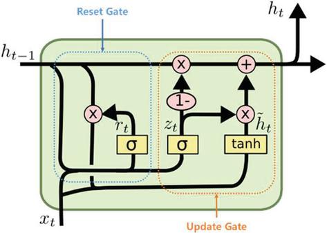
Figure 3 GRU cell state [10, 11].
It is Equation (9) which is needed to calculate a reset gate. In this equation, the previous hidden state and current ‘’ were calculated with the activation function ‘sigmoid’. The results would range from ‘0’ to ‘1’ and can be interpreted as how much the previous hidden state would be used. Instead of using the value from the reset gate as it is, Equation (10) is applied. In this equation, the previous hidden state is multiplied by a reset gate.
The update gate is similar to LSTM’s input and forget gates in terms of role. It is key to calculate the ratio of past and current data to be reflected. With the result ‘’ acquired through Equation (11), how much current data would be used is decided. Furthermore, how much past data would be used is decided with ‘()’. Therefore, each role can be viewed as LSTM’s input/forget gate. Lastly, a current hidden state can be estimated through Equation (12):
| (9) | ||
| (10) | ||
| (11) | ||
| (12) |
Compared to conventional LSTM, GRU is further simpler. In terms of performances, it is not better than LSTM. However, GRU has fewer parameters to learn.
2.4 Performance Metrics
In this study, room mean square error (RMES) [12] and mean absolute percentage error (MAPE) [12] are used to assess the accuracy of model prediction more precisely.
RMSE is commonly used to handle a difference between model predictions and observations, and the results are acquired as shown in Equation (13) below:
| (13) |
MAPE is an index which represents the percentage of a difference between actual values and predictions to actual ones, and it can be calculated as shown in Equation (14). A model with smaller error mean is deemed good. In RMSE, unless data are normalized, there is a problem in the outlier. In MAPE, on the contrary, performances are reflected on the outlier.
In terms of the disadvantages of the MAPE, if the actual value is (or is close to) ‘0’, an error becomes infinite at a particular instance, increasing an error scale dramatically.
| (14) |
3 Experiments
3.1 Data Description and Experiment Design
The data used in this study were collected from 26 different circuits among the backbone and subscribers of Korea Research Environment Open Network (KREONET) [13]. Here, KREONET refers to a research network that supports the development of science and technology in Korea. Specifically, a total of 2,762,734 data records collected every 5 minutes from July 8, 2020 to July 11, 2021 were used. Since data in each circuit revealed their own patterns, datasets were made by connecting such 26 circuits to learn data in diverse patterns. The attributes and definitions are the collected data were shown in Figure 4. Because almost no data were lost during collection, the lost ones were estimated, using pre-data with the closest time.
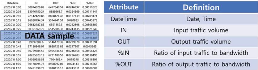
Figure 4 Data definition and sample.
For processing the inputs of a machine-learning model, data for the past seven days were defined with a single instance. A single instance is defined in 8,064 dimensions, including ‘12 (No. of data records collected per hour) 24 (hours) 4 (No. of attributes) 7 (days)’. Each instance was processed to get Max_In, Max_Out, Max%In and Max%Out attributes by calculating maximum daily traffic.
For learning and verification, original data were split in a 7:3 ratio, and 6,578 learning datasets were divided into 2,834 verification datasets.
In a machine-learning model, SVR, LSTM and GRU were used. For model optimization, experiments were performed multiple times. At first, to see the trend, the learning rate was set to 0.0001, epoch 1000, and hidden size 1000, and the experiment was conducted by changing the sliding window to 1, 3, 5, 7, 14. The experiment was performed by fixing the sliding Windows 7 with the best performance, changing the learning rate to 0.1, 0.01, 0.001, 0.0001, 0.0001, and the epoch to 100, 500, 1000, and 2000. Then, the experiment was conducted by fixing the sliding Windows 7, learning rate 0.0001, epoch 1000, and changing the hidden size to 500, 1000, 2000, 3000, 4000, and 5000. As a result, sliding window size, learning rate, hidden state size and epoch were set to ‘7 days’, ‘0.0001’, ‘3,000’ and ‘1,000’ respectively.
Table 1 SVR, LSTM, GRU model evaluation result in total data set
| SVR | LSTM | GRU | |
| IN | 0.4281 G | 0.2690 G | 0.2936 G |
| OUT | 0.4918 G | 0.4159 G | 0.4077 G |
| %IN | 4.9357 % | 4.1990 % | 4.2725 % |
| %OUT | 5.5082 % | 5.2485 % | 5.3289 % |
3.2 Experimental Results
The results obtained through RMSE after learning total data with three different models (SVR, LSTM, GRU) were stated on Table 1. The table reveals that except for ‘OUT’, LSTM showed the best performances. ‘IN’ and ‘OUT’ revealed ‘95% or higher’ and ‘94% or higher’ respectively. A prediction error (200–400 Mbps) is found at 10 Gbps in general due to a backbone section. Therefore, it appears that no particular issue would occur when actual traffic engineering is applied. However, it is ‘the Catch in Average’ which should be considered. In average, a prediction error remains at around 5% against bandwidth, but it could get worse. This issue would be handled later.
Figure 5 is the results of the prediction of the backbone circuit A(Daejeon-Seoul) traffic, using LSTM which showed the best learning results. In terms of the results of Figure 5, RMSE was 0.0991 at IN traffic in the backbone circuit A(Daejeon-Seoul), showing about 100 Mbps mean error. In addition, MAPE which represents a prediction error ratio was 0.0981, revealing about 10% error against actual traffic. Similar results were observed even at OUT traffic. Since a backbone section is an area where traffic from multiple subscribers is combined, good results with a constant pattern are expected.
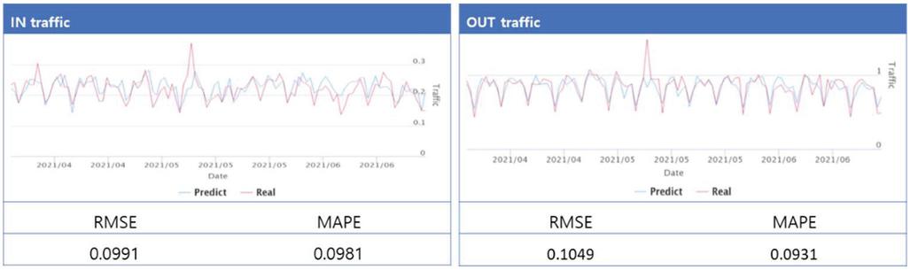
Figure 5 Prediction and evaluation result (backbone circuit A(Daejeon-Seoul)).
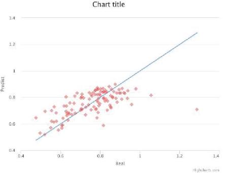
Figure 6 Distribution of predicted and actual values (Seoul-Daejeon Circuit).
In Figure 6, a ‘’ linear function graph was added to the distribution of predictions and actual values. As red dots got closer to the blue line, prediction was more accurate. When ‘the Catch in Average’ was mentioned, red dots off from the blue line were observed in Figure 6 below. Since such dots have small numbers, the results might look good. As shown in red dots at the left bottom, it is able to create congestion in the backbone through traffic engineering with incorrect predictions
Figure 7 shows the results of the circuit of Kyungbuk National University, one of KREONET subscribers. According to IN traffic RMSE, a 0.0655 (approx. 65 Mbps) mean error can be confirmed. In addition, MAPE was 0.2254, predicting about 22% error in average. While RMSE is low, MAPE would be higher because of small bandwidth. The subscriber’s traffic against backbone, an error can be large due to significant variation per each agency’s characteristics.
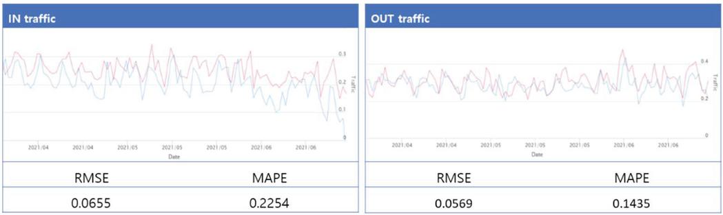
Figure 7 Prediction and evaluation result (Kyungbuk University Circuit).
Based on the above experiments, this study predicted maximum traffic on the following day through a percentage of traffic to traffic volume and bandwidth. In a backbone zone, an error of nearly 10% or less was obtained. In addition, it is difficult to collect flow data on an Internet service provider (ISP)-scale network. However, it is relatively simple to collect traffic volume [14, 15]. Hence, it might be fairly easy to apply the discussed prediction methods to actual fields. It is anticipated that this study would help network operators handle traffic engineering by predicting maximum traffic on the following day.
4 Conclusion
This study used a traffic volume-based prediction method to maximize the efficiency of network operation through the creation of easy datasets and traffic prediction. In terms of a more practical plan, this study predicted, using traffic volume for easy data collection. To enhance utilization in traffic engineering, this study predicted maximum traffic on the following day, showing a nearly 10% error on a backbone zone.
Previous studies had problems with increasing accuracy by predicting traffic in the short future, or low accuracy when predicting the future for 24 hours. In this study, the accuracy could be improved because one value was predicted by predicting the maximum value of traffic for 24 hours.
There might be further studies on how to improve accuracy by collecting and learning circuits with high similarities by clustering each circuit according to characteristics. In terms of further studies, each circuit would be clustered through clustering techniques such as K-means [16]. Then, there have been studies to enhance accuracy by collecting and learning circuits with great similarities, helping clusters learn from each other. It is anticipated that there would be continued studies on a KREONET backbone through connection with more accurate KREOENT-S’ virtually dedicated network (VDN) [17] in connection with the technology to dynamically allocate circuits.
Acknowledgements
This research was supported by Korea Institute of Science and Technology Information (KISTI).
References
[1] Huifang Feng, Yantai Shu, ‘Study on Network Traffic Prediction Techniques’, International Conference on Wireless Communications, Networking and Mobile Computing, pp. 1041–1044, 2005
[2] Vinayakumar R, Soman KP, et al., ‘Applying Deep Learning Approaches for Network Traffic Prediction’, ICACCI, 2353–2358, 2017
[3] Paulo Cortez, Miguel Rio, et al., ‘Internet Traffic Forecasting using Neural Networks’, International Joint Conference on Neural Networks, pp. 2635–2642, 2006
[4] Nandini Krishnaswamy, Mariam Kiran, ‘Data-driven Learning to Predict WAN Network Traffic’, SNTA, pp. 11–18, 2020
[5] Harris Drucker, Chirs J.C. Buges., et al., ‘Support Vector Regression Machines’, Advances in neural information processing systems 9, pp. 155–161, 1996
[6] Chi-Jie Lu a, Tian-Shyug Lee, et al., ‘Financial time series forecasting using independent component analysis and support vector regression’, Decision Support Systems, pp. 115–125, 2009
[7] Sepp Hochreiter, Jürgen Schmidhuber, ‘Long Short-term Memory’, Neural Computation, pp. 1735–1780, 1997
[8] Dejun Chen, Congcong Xiong, et al., ‘Improved LSTM Based on Attention Mechanism for Short-term Traffic Flow Prediction’, 10th International Conference on Information Science and Technology, pp. 71–76, 2020
[9] W. Esmail, T. Stockmanns, et al., ‘Machine Learning for Track Finding at PANDA’, Proceedings of the CTD/WIT, pp, 2019
[10] Kyunghyun Cho, et al., ‘Learning Phrase Representations using RNN Encoder-Decoder for Statistical Machine Translation’, EMNLP 2014, pp. 1724–1734, 2014
[11] Rui Fu, Zuo Zhang, and Li Li, ‘Using LSTM and GRU Neural Network Methods for Traffic Flow Prediction’, 2016 31st Youth Academic Annual Conference of Chinese Association of Automation (YAC), pp. 324–328, 2016
[12] Rob J. Hyndman, et al., ‘Another look at measures of forecast accuracy’, International Journal of Forecasting 22, pp. 697–688, 2006
[13] The KREONET official website http://www.kreonet.net/kreonet/index.jsp
[14] William Stallings, ‘SNMP and SNMPv2: The Infrastructure for Network Management’, IEEE Communications Magazine, pp. 37–43, 1998
[15] Tobias Oetiker, ‘MRTG – The Multi Router Traffic Grapher’, 1998
[16] D. Arthur, S. Vassilvitskii, ‘How Slow is the k-means Method?’ Proceedings of the 2006 Symposium on Computational Geometry, 2006
[17] Yong-hwan Kim, Ki-Hyeon Kim, Dongkyun Kim, ‘Design and Implementation of Virtually Dedicated Network Service in SD-WAN Based Advanced Research & Educational (R&E) Network’, The Journal of Korean Institute of Communications and Information Sciences, pp. 2050–2064, 2017
Biographies
Chanjin Park received the master’s degree in computer engineering from Sungkyunkwan University in 2010, From 2012 to 2015, he has been a officer in Korea Military Academy, Seoul, Korea. And since 2015, he has been a engineer in Korea Institute of Science & Technology Information (KISTI), Daejon, Korea. His research area include network management, security, measurement and machine learning.
Wonhyuk Lee received his Ph. D. degree in the department of computer engineering from Sungkyunkwan University, Korea, in 2010. Since 2003, he has been a senior engineer in Korea Institute of Science & Technology Information (KISTI), Daejon, Korea. His research interests include network management, security, measurement and next generation network.
Moon-Hyun Kim received the B.S. degree in Electronic Engineering from Seoul National University in 1978, the M.S. degree in Electrical Engineering from Korea Advanced Institute of Science and Technology, Korea, in 1980, and the Ph.D. degree in Computer Engineering from the University of Southern California in 1988. From 1980 to 1983, he was a Research Engineer at the Daewoo Heavy Industries Co., Seoul. He joined College of Software, Sungkyunkwan University, Seoul, Korea in 1988, where he is currently a an emeritus professor. In 1995, he was a Visiting Scientist at the IBM Almaden Research Center, San Jose, California. In 1997, he was a Visiting Professor at the Signal Processing Laboratory of Princeton University, Princeton, New Jersey. His research interests include artificial intelligence, machine learning and pattern recognition.
Ung-Mo Kim received the bachelor’s degree in Mathematics from Sungkyunkwan University in 1981, the master’s degree in computer science from Old Dominion University in 1986, and the philosophy of doctorate degree in computer science from Northwestern University in 1990, respectively. He is currently working as a Full Professor at the College of Computing and Informatics, Sungkyunkwan University. His research areas include Database, Data Mining, Big Data.
Taehong Kim received his M.S. and Ph.D. degrees from the Department of Applied Information Science at University of Science and Technology in 2010 and 2014, respectively. After graduation, he has conducted researches on Semantic Web, Big Data, and IoT in Korea Institute of Science and Technology Information until 2018. After that, he has expanded his research area to Korean medicine informatics in Korea Institute of Oriental Medicine. His research areas include person-generated health data, time-series data, and medical data analysis.
Seunghae Kim received the BS degees from the Hannam University, Korea and the MS and the PhD degrees from the Jeonbuk National University, Korea. He is currently a Network Engineer and Principal Reseacher at the Korea Institute Science and Technology Information. His research interests include Network architecture, Network security, Routing and Network Operation.
Journal of Web Engineering, Vol. 21_5, 1419–1434.
doi: 10.13052/jwe1540-9589.2152
© 2022 River Publishers