Microservices Identification in Monolith Systems: Functionality Redesign Complexity and Evaluation of Similarity Measures

Samuel Santos and António Rito Silva^*

INESC-ID, Department of Computer Science and Engineering, Instituto Superior Técnico, University of Lisbon
E-mail: samuel.c.santos@tecnico.ulisboa.pt; rito.silva@tecnico.ulisboa.pt
*Corresponding Author

Received 08 October 2021; Accepted 03 June 2022; Publication 05 August 2022

Abstract

As monolithic applications grow in size and complexity, they tend to show symptoms of monolithic hell, such as scalability and maintainability problems. To help suppressing these problems, the microservices architectural style is applied. However, identifying the services within the monolith is not an easy task, and current research approaches emphasize different qualities of microservices. In this paper we present an approach for the automatic identification of microservices, which minimizes the cost of the monolith’s functionalities redesign. The decompositions are generated based on similarity measures between the persistent domain entities of the monolith. An extensive analysis of the decompositions generated for 121 monolith systems is done. As result of the analysis we conclude that there is not a similarity measure, neither a combination of similarity measures, that provides better decomposition results in terms of complexity associated with the functionalities migration. However, we prove that it is possible to follow an incremental migration process of monoliths. Additionally, we conclude that there is a positive correlation between coupling and complexity, and that it is not possible to conclude on the existence of a correlation between cohesion and complexity.

Keywords: Microservices architecture, microservices identification, static code analysis, software architecture.

1 Introduction

Companies like Amazon and Netflix [28] faced constraints on the evolution of their monolith systems, due to the coupling resulting from the use of a large domain model maintained in a shared database. As monolithic applications grow in size, they easily become too large and complex to be managed: the implementation of new functionalities becomes slower, there is less awareness on the impact of changing one piece of code, and the overall deployment becomes more difficult.

To address these problems, microservices [11] have become the architecture of choice to the development of large scale and complex systems. It supports the split of a large development team into several agile ones, and the independent development, deployment and scalability of services. However, the adoption of this architectural style is not free of problems [36], where the identification of microservices boundaries is one of the most challenging, which may require an expert with in-depth knowledge of the application. Furthermore, architects may identify services that, although with good indicators of commonly considered attributes in microservices research, such as high cohesion and low coupling, require more changes in the application’s business logic when migrating to a microservices architecture style.

Note that, when migrating into microservices, functionalities that were executed atomically, according to the ACID properties of transactions, may become split into several distributed transactions. The ACID transactional context generate a semantic coupling between domain entities accessed in the context of a functionality, which simplifies its implementation. Nevertheless, when the functionality is redesigned in the microservices architecture it is necessary to consider the relaxing of consistency, where the entities accessed by the functionality can have visible intermediate states during the functionality execution, according to the CAP theorem [12]. This aspect has been mainly ignored in the proposals for the migration of monolith systems to microservices, problem known as Forgetting about the CAP Theorem [7].

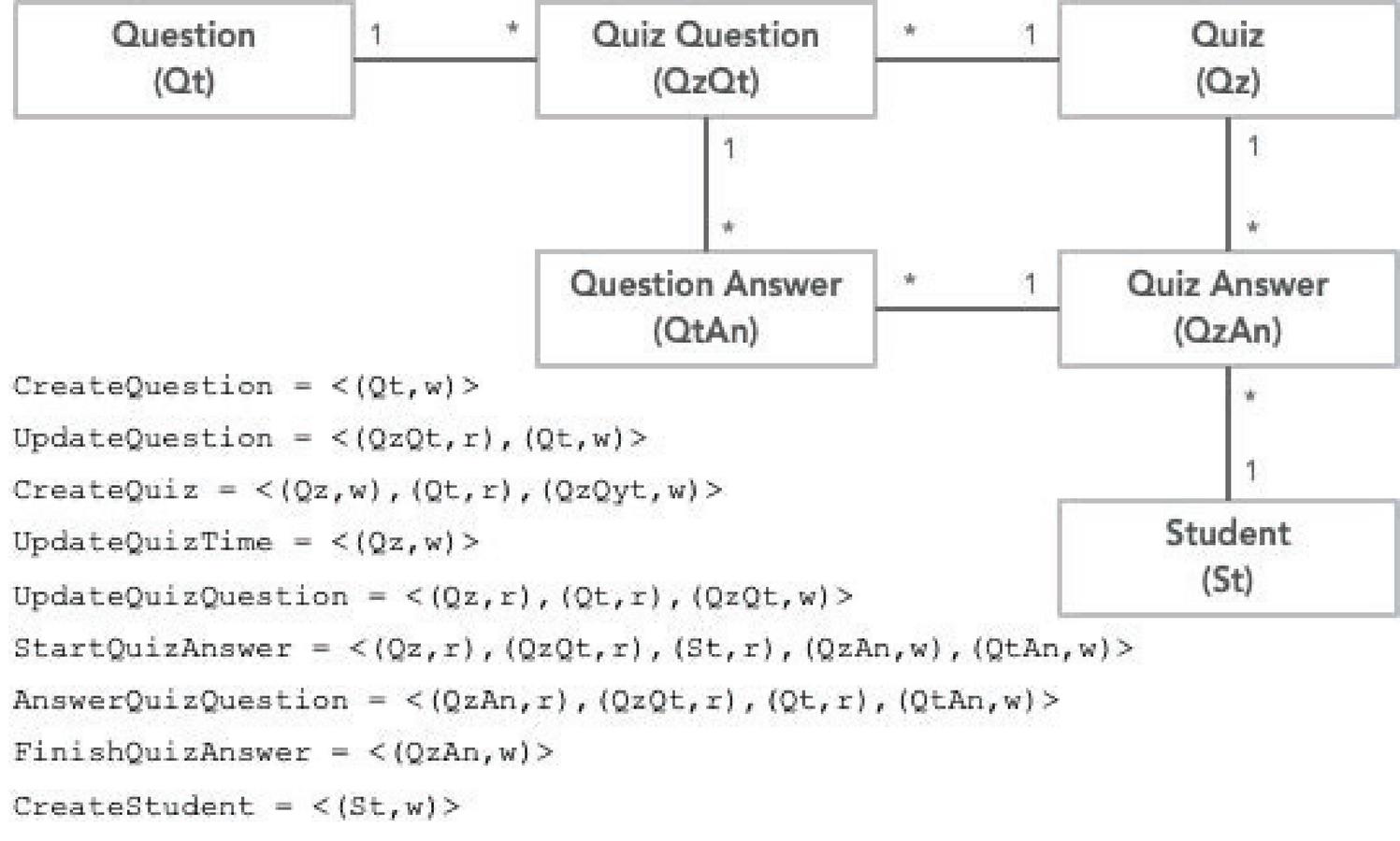
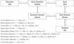
Figure 1 Quizzes Domain Model and Functionalities, described as sequences of read (r) and write (w) accesses on the domain entities.

Consider the domain model in Figure 1 for a online Quizzes system with the associated functionalities. The functionalities are described as sequences of reads and writes on the domain entities. The challenge is to identify a decomposition which minimize the complexity of distributed transactions. For instance, if Question and Student entities are associated with their own microservices, functionalities CreateQuestion and CreateStudent continue to be ACID, because they execute in a single microservice. On the other hand, more complex functionalities, like StartQuizAnswer, have to be implemented using several distributed transactions, but a way to minimize their complexity is to have a single write transaction. In the case of StartQuizAnswer the best strategy would be to include entities QuestionAnswer and QuizAnswer in the same microservice.

These are the type of strategies of follow to identify microservices, but considering that a monolith can have dozens of domain entities and hundreds of functionalities the identification of microservices on monolith systems requires some sort of automation.

The research on the automatic, or semi-automatic, microservices boundaries identification in monolith systems, e.g. [3, 13, 37, 19], take advantage of the monolith’s codebase and runtime behavior to collect data, analyse it, and propose a decomposition of the monolith. Although each of the approaches use different techniques, they follow the same basic three phases: (1) Collection: collect data from the monolith system; (2) Decomposition: define a decomposition by applying a similarity measure and an aggregation algorithm, like a clustering algorithm, to the data collected in the first phase; (3) Analysis: evaluate the quality of the generated decomposition using a set of metrics.

Our analysis framework is built on top of what is considered by the gray literature as one of the main difficulties on the identification of microservices boundaries in monolith systems: the transactional contexts [10, Chapter 5]. [27] proposes an approach to the identification of microservices that is driven by the transactional contexts where they are executed, using similarity measures between domain entities inferred from the functionalities that access them, instead of their structural domain inter-relationships.

For instance, considering the example in Figure 1 the similarity measure between QuestionAnswer and QuizAnswer should be higher, than between QuestionAnswer and Student, because they are accessed more frequently by the same functionalities, and it is also relevant that in some functionalities they are written together. Entities that have a higher similarity measure will tend to be included in the same decomposition.

Additionally, [34] proposes a complexity metric that measures the redesign cost of the monolith functionalities, due to the lack of isolation between the execution of the distributed transactions. For instance, when redesigning functionality StartQuizAnswer, which reads QuizQuestion, it is necessary to analyse all the functionalities that change the values the functionality reads, like functionality UpdateQuizQuestion, which writes QuizQuestion, to guarantee that the reads are kept consistent.

We leverage on the previous work by broadening its scope, because of the larger number of monolith implementations that are supported, Spring Data JPA. Additionally, we do an extensive analysis of 121 monolith systems to study whether variations on the application of the approach provide significant differences when identifying candidate decompositions.

In this section we defined the context of our work. Next section outlines the overall approach, and Section 3 formalizes our analysis framework. Section 4 describes our collection tool’s implementation and Section 5 presents an extensive analysis over 121 systems. The related work on the migration to microservices is presented in Sections 6 and 7 discusses the lessons learned, threads to validity and future work. Finally, Section 8 concludes the paper with final remarks and an overall summary of our work.

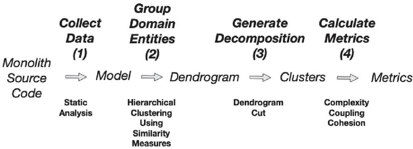
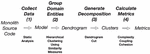
Figure 2 Processing pipeline.

2 Approach

In this paper, we propose a processing pipeline for the identification of microservices in a monolith system, which is described in Figure 2:

• Collect Data (1): A static analysis tool is applied to the monolith source code to generate a model of the monolith. This model contains the sequences of accesses, read and write, that each of the monolith functionalities does on the persistent domain entities;

• Group Domain Entities (2): Afterwards, the model is used to calculate a set of similarity measures, among the persistent domain entities, that are used to group them such that the resulting decomposition minimizes the number of distributed transactions in the microservices implementation of the monolith functionalities. According to these similarity measures two domain entities are closer if they are frequently accessed by the same functionalities. A hierarchical clustering algorithm is applied to generate a dendrogram;

• Generate Decomposition (3): The dendrogram is cut to generate a decomposition with a particular number of domain entities clusters;

• Calculate Metrics (4): Three metrics are applied to the decomposition generated in the previous phase: complexity; cohesion; and coupling. Complexity measures the cost associated with the implementation of monolith functionalities as distributed transactions. Cohesion measures whether the functionalities accesses to a cluster follow the single responsibility principle: all cluster domain entities are accessed. Finally, coupling measures the number of domain entities that a cluster exposes to another cluster, which is inferred from the functionalities accesses among clusters.

As an example, consider a monolith that as 4 domain entities, $e_{1}, e_{2}, e_{3}$ and $e_{4}$ , and two functionalities, $f_{1}$ and $f_{2}$ , where $f_{1}$ sequence of access is $< (e_{1}, r), (e_{2}, w), (e_{3}, r) >$ and $f_{2}$ sequence of accesses is $< (e_{3}, r), (e_{4}, w) >$ . These sequences of accesses are part of the model that is obtained in phase 1 of the processing pipeline. In terms of similarity distance, $e_{1}$ is closer to $e_{2}$ than to $e_{4}$ , because they are in the same functionality. Therefore, after applying steps 2 and 3, a decomposition having two clusters would be $c_{1} = {e_{1}, e_{2}, e_{3}}$ and $c_{2} = {e_{4}}$ . Given this decomposition, in terms of complexity, which is calculated in phase 4, $f_{1}$ can be implemented as an ACID transaction, since it only accesses $c_{1}$ (implemented by a single microservice) but the complexity of $f_{2}$ will be higher because it becomes a distributed transaction that has to do a read on $c_{1}$ and a write on $c_{2}$ (implemented by two microservices). Note that the $f_{1}$ is implemented by a single local transaction, whereas $f_{2}$ is implemented by two, $l_{1} = < (e_{3}, r) >$ and $l_{2} = < (e_{4}, w) >$ , and the pair $r i = ((e_{3}, r), (e_{4}, w))$ represents a remote invocation between them.

Finally, we analyse the performance of different combinations of similarity measures in terms of the 3 metrics, and assess whether the decompositions that minimize the transactional complexity also tend to provide good results in terms of modularity: cohesion and coupling. This evaluation is done by generating, for the 121 codebases, the decompositions resulting from the all combinations of the similarity measures, and doing a statistical analysis of the results.

3 Monolith Decomposition

A monolith is defined by its set of functionalities which execute in atomic transactional contexts and, due to the migration to the microservices architecture, have to be decoupled into a set of distributed transactions, each one executing in the context of a microservice.

Therefore, a monolith is defined as a triple $(F, E, G)$ , where $F$ defines its set of functionalities, $E$ the set of domain entities, and $G$ a set of call graphs, one for each monolith functionality. A call graph is defined as a tuple $(A, P)$ , where $A = E \times M$ is a set of read and write of accesses to domain entities ( $M = {r, w}$ ), and $P = A \times A$ a precedence relation between elements of $A$ such that each access has zero or one immediate predecessors, $\forall_{a \in A} # {(a_{1}, a_{2}) \in P : a_{1} = a} \leq 1$ , and there are no circularities, $\forall_{(a_{1}, a_{2}) \in P_{T}} (a_{2}, a_{1}) \notin P_{T}$ , where $P_{T}$ is the transitive closure of $P$ . The precedence relation represents the sequences of accesses associated with a functionality.

Considering the previous example, the accesses and their sequences define the set of call graphs $G$ , one call graph for each functionality.

3.1 Similarity Measures

The definition of similarity measures establishes the distance between domain entities. Domain entities that are closer, according to a particular similarity measure, should be in the same microservice. Therefore, since we are interested in reducing the number of distributed transactions a functionality is decomposed in, we intend to define as close the domain entities that are accessed by the same functionalities.

The access similarity measure measures the distance between two domain entities, $e_{i}, e_{j} \in E$ , as:

s m_{a c c e s s} (e_{i}, e_{j}) = \frac{# (f u n c t (e_{i}) \cap f u n c t (e_{j}))}{# f u n c t (e_{i})}

where $f u n c t (e)$ denotes the set of functionalities in the monolith whose call graph has a read or write access to $e$ . This measure takes a value in the interval 0..1. When all the functionalities that access $e_{i}$ also access $e_{j}$ then it takes the value 1.

For instance, considering the previous example, $s m_{a c c e s s} (e_{2}, e_{3}) = 1$ , because only $f_{1}$ accesses both entities, but $s m_{a c c e s s} (e_{3}, e_{2}) = 1 / 2$ , because the two functionalities access $e_{3}$ .

Since the cost of reading and writing is different in the context of distributed transactions, because writes introduce new intermediate states in the decomposition of a functionality [14], the next two similarity measures distinguish read from write accesses in order to reduce the number of write distributed transactions:

$s m_{r e a d} (e_{i}, e_{j})$	$= \frac{# (f u n c t (e_{i}, r) \cap f u n c t (e_{j}, r))}{# f u n c t (e_{i}, r)}$
$s m_{w r i t e} (e_{i}, e_{j})$	$= \frac{# (f u n c t (e_{i}, w) \cap f u n c t (e_{j}, w))}{# f u n c t (e_{i}, w)}$

where $f u n c t (e, m)$ denotes the set of functionalities in the monolith whose call graph has an access according to mode $m$ , read or write, respectively. These two measures tend to include in the same microservice, domain entities that are read or written together, respectively.

For instance, considering the previous example, $s m_{r e a d} (e_{2}, e_{3}) = 0$ and $s m_{w r i t e} (e_{2}, e_{3}) = 0$ , because they do not have common reads neither common writes in the same functionalities.

Finally, another similarity measure that is found in the literature groups domain entities that are frequently accessed in sequence, in order to reduce the number of remote invocations between microservices, i.e., the domain entities that are frequently accessed in sequence should be in the same microservice. Therefore, the sequence similarity measure is defined:

s m_{s e q u e n c e} (e_{i}, e_{j}) = \frac{s u m P a i r s (e_{i}, e_{j})}{m a x P a i r s}

where $s u m P a i r s (e_{i}, e_{j}) = \sum_{f \in F} # {(a_{k}, a_{m}) \in G_{f} . P : (a_{k} . e = e_{i} \land a_{m} . e = e_{j}) \lor (a_{k} . e = e_{j} \land a_{m} . e = e_{i})})$ , where $G_{f} . P$ is the precedence relation for functionality $f$ , is the number of consecutive accesses of $e_{i}$ and $e_{j}$ , and $m a x P a i r s = m a x_{e_{k}, e_{m} \in E} (s u m P a i r s (e_{k}, e_{m}))$ is the max number of consecutive accesses for two domain entities in the monolith.

In what concerns the sequence similarity measure, $s m_{s e q u e n c e} (e_{2}, e_{3}) = 1$ , because there is a pair, $< (e_{2}, w), (e_{3}, r) >$ , and the max number of pairs is also 1.

3.2 Complexity Metric

A decomposition of a monolith is a partition of its domain entities set, where each element is included in exactly one subset, a cluster, and a partition of the call graph of each one of its functionalities. Therefore, given the call graph $G_{f}$ of a functionality $f$ , and a decomposition $D \subseteq 2^{E}$ , the partition call graph of a functionality $p a r t i t i o n (G_{f}, D) = (L T, R I)$ is defined by a set of local transactions $L T$ and a set of remote invocations $R I$ , where each local transaction

1. is a subgraph of the functionality call graph, $\forall_{l t \in L T} : l t . A \subseteq G_{f} . A \land l t . P \subseteq G_{f} . P$ ;

2. contains only accesses in a single cluster of the domain entities decomposition, $\forall_{l t \in L T} \exists_{c i n D} : l t . A . e \subseteq c$ ;

3. contains all consecutive accesses in the same cluster, $\forall_{a_{i} \in l t . A, a_{j} \in G_{f} . A} : ((a_{i} . e . c = a_{j} . e . c \land (a_{i}, a_{j}) \in G_{f} . P) ⟹ (a_{i}, a_{j}) \in l t . P) \lor ((a_{i} . e . c = a_{j} . e . c \land (a_{j}, a_{i}) \in G_{f} . P) ⟹ (a_{j}, a_{i}) \in l t . P)$ .

From the definition of local transaction, results the definition of remote invocations, which are the elements in the precedence relation that belong to different clusters, $R I = {(a_{i}, a_{j}) \in G_{f} . P : a_{i} . e . c \neq a_{j} . e . c}$ . Note that, in these definitions, we use the dot notation to refer to elements of a composite or one of its properties, e.g., in $a_{j} . e . c$ , $. e$ denotes the domain entity in the access, and $. c$ the cluster the domain entity belongs to.

The complexity for a functionality migration, in the context of a decomposition, is the effort required in the functionality redesign, because its transactional behavior is split into several distributed transactions, which introduce intermediate states due to the lack of isolation. Therefore, the following aspects have impact on the functionality migration redesign effort:

• The number of local transactions, because each local transaction may introduce an intermediate state;

• The number of other functionalities that read domain entities written by the functionality, because it adds the need to consider the intermediate states between the execution of the different local transactions;

• The number of other functionalities that write domain entities read by the functionality, because the functionality redesign has to consider the different states these domain entities can be.

This complexity is associated with the cognitive load that the software developer has to address when redesigning a functionality. Therefore, the complexity metric is defined in terms of the functionality redesign.

c o m p l e x i t y (f, D) = \sum_{l t \in p a r t i t i o n (G_{f}, D)} c o m p l e x i t y (l t, D)

The complexity of a functionality is the sum of the complexities of its local transactions.

c o m p l e x i t y (l t, D)

= # \cup_{a_{i} \in p r u n e (l t)} {f_{i} \neq l t . f : d i s t (f_{i}, D) \land a_{i}^{- 1} \in p r u n e (f_{i}, D))}

The complexity of a local transaction is the number of other distributed functionalities that read, or write, domain entities, written, or read, respectively by the local transaction. The auxiliary function $d i s t$ identifies distributed functionalities, given the decomposition; $a_{i}^{- 1}$ denotes the inverse access, e.g. ${(e_{i}, r)}^{- 1} = (e_{i}, w)$ ; and $p r u n e$ denotes the relevant accesses inside a local transaction, by removing repeated accesses of the same mode to a domain entity. If both read and write accesses occur inside the same local transaction, they are both considered if the read occurs before the write. Otherwise, only the write access is considered. These are the only accesses that have impact outside the local transaction.

Considering the example, the complexity of functionality $f_{1}$ is equal to the complexity of its single local transaction, which is 0, because $f_{2}$ does not write any of the entities read by $f_{1}$ . On the other hand, the complexity of $f_{2}$ is equal to the sum of the complexities of its two local transactions. But, since $f_{1}$ is not a distributed functionality, and considering only these two functionalities, both local transactions of $f_{2}$ have complexity 0. Note that, in this example is not necessary to apply the prune function, because the sequences do not access the same entity more than once.

3.3 Cohesion and Coupling Metrics

Cohesion and coupling are important qualities of any software system, particularly, in a system implementing a microservices architecture, because one of its goals is to foster independent agile teams. Therefore, we intend to measure the cohesion and coupling of the monolith decomposition.

The cohesion of a cluster of domain entities depends on the percentage of its entities that is accessed by a functionality. If all the cluster’s assigned entities are accessed each time a cluster is accessed, it means that the cluster is cohesive:

c o h e s i o n (c) = \frac{\sum_{f \in f u n c t (c)} \frac{# {e \in c . e : e \in G_{f} . A . e}}{# c . e}}{# f u n c t (c)}

where $f u n c t (c)$ denotes the functionalities that access the cluster $c$ , and $G_{f} . A . e$ the entities that are accessed by functionality $f$ .

The coupling between two clusters is defined by the percentage of entities one cluster exposes to other cluster. It can be defined in terms of the remote invocations between the two clusters.

c o u p l i n g (c_{i}, c_{j}) = \frac{# {e \in c_{j} : \exists_{r i \in R I (c_{i}, c_{j})} e = r i [2] . e}}{# c_{j} . e}

where $R I (c_{i}, c_{j})$ denotes the remote invocations from cluster $c_{i}$ to cluster $c_{j}$ .

4 Solution

In the collection phase, the data collection tool is implemented using Spoon [29] to introspect codebases that use different technologies. The goal is to collect data from a significantly higher number of codebases and use them in the evaluation.

The collection phase produces, for each analyzed monolith, a JSON file that contains the functionalities accesses. This file consists in a key-value store that maps the functionality name to a list of all the accesses to domain entities, in depth-first search order, that can possibly be made in the context of the functionality execution.

During the decomposition phase of the migration process, the tool uses hierarchical clustering (Python SciPy¹) to process the collected data and, according to the 4 similarity measures, generate a dendrogram of the domain entities. The generated dendrogram can then be cut in order to produce different decompositions, given a number of clusters. The decomposition tool supports all different combinations of the similarity measures, with intervals of 10% and where the sum of the percentage of similarity measures should be equal to 100%. For instance, a dendrogram is generated for the following weights, 30% access, 30% read, 20% write, 20% sequence, because each value is a multiple of 10 and the sum is 100. Then, each dendrogram is cut to generate multiple decompositions, varying the number of clusters.

In the analysis phase the tool compares the multiple generated decompositions according to the three quality metrics: complexity, coupling and cohesion.

4.1 Object-Relational Mapper Frameworks

The collection tool is configured to collect data from monolith applications implemented using Spring Boot² and two Object-Relational Mappers (ORMs), FenixFramework³ and Hibernate.⁴

FenixFramework is an ORM that supports rich domain-models using software transactional memory [6]. It was chosen because we are familiar with it and provides a complete object-oriented interface that hides the database structure. Hibernate is a well known implementation of the JPA specification [21]. Comparing to two other popular JPA providers, Eclipse Link⁵ and OpenJPA,⁶ Hibernate has a significantly bigger community, better documentation and is more widely used and, thus, a better option to be considered.

In codebases that exclusively use Hibernate mechanisms, the interaction with the persistence context is done via the EntityManager interface, however, this interface provides lots of different ways to create queries and access the database. Furthermore, codebases that do not follow a consistent design pattern can call the data access methods from anywhere in the code, with data coming from different places (arguments, constants, variables, return values of function calls, etc.), which hampers the static analysis process. Therefore, we decided to only consider codebases that, besides using Hibernate ORM, also implement the Repository Pattern [24] and exclusively use Spring Data JPA⁷ repositories to access the database.

This pattern significantly facilitates the static analysis process, since we only need to identify the repository classes, identify calls to its methods when analysing the accesses made in the functionality call-graph, and infer the persistent domain entities that are being accessed.

4.2 Data Collection

As said, the analysed monoliths are implemented using the popular Java Spring Boot framework that follows the Model-View-Controller architecture [23]. Therefore, each monolith’s functionality has its entry point implemented in well-known classes, which are the controller classes. In Spring Boot, these classes are annotated with specific annotations, such as the @Controller annotation, and may implement methods that, when annotated with spring mapping annotations (such as @RequestMapping), map web requests to Spring Controller methods, triggering the transactional execution of a functionality.

Regarding the identification of the accesses to the persistent domain entities, in FenixFramework it is only possible to access the database through calls to methods implemented by FenixFramework generated classes. After specifying the entities to be persisted and the relationships they possess, FenixFramework generates the code and makes each domain entity inherit from classes that implement the data access methods, which can then be called in the subclasses, which contain the domain entities business logic. The names of the FenixFramework generated classes and respective methods follow a specific nomenclature, which allows the identification of the type of accesses and the entities being accessed. The methods that read entity relationships always start with get and the ones that write/update a relationship always start with either set, add, or, remove. Additionally, there is the static method in the FenixFramework class, getDomainObject, that materializes a domain entity from the database, given its unique identifier.

In Hibernate JPA, persistent domain entities are annotated with the @Entity annotation and always have a corresponding database table, and the accesses to the persistent context can be made in two ways.

The first way is through the use of HQL⁸ or SQL queries declared in the repository classes. It is possible to annotate repository methods with the @Query annotation and explicitly indicate which query should be executed when the method is called. This forces us to identify the database tables that are associated to the domain entities and referenced by the repository queries to infer which entities are accessed. Each domain entity in Hibernate is mapped to a database table with the same name of the entity (by default). Other tables can also be created when declaring relationships between entities through the use of annotations and annotation values, e.g, @OneToMany and @ManyToMany. The generated tables can either be explicitly named through the use of annotation values or follow the Hibernate’s default naming strategy. Additionally, we also need to identify named queries. Named queries are static queries that can be declared in @Entity classes through the use of annotations, and that can be referenced by repositories by declaring a method whose name is identical to the name of the named query.

The second way of accessing the persistent domain entities in Hibernate follow a more object-oriented style. It is through calls that access associations between domain entities that have not been loaded yet. Hibernate allows to specify whether a relationship should be loaded eagerly or lazily when an object is retrieved from the database, thus, calling, for instance, a getter of an entity that has an association to another domain entity may potentially result in the load (access) of the second entity from the database. In our implementation we consider that all the relationships are lazily fetched. This is a better approach to identify the actual transactional context of each functionality, since we will only consider the entities that are strictly used. For example, if there’s a functionality that retrieves an entity with eager fetch configured on all its associations, but only accesses some of them, only the accessed domain entities are considered and the others are discarded, even though they were materialized in memory during the execution of the functionality.

Therefore, the data collection tool implemented in Spoon follows the steps (FO stands for FenixFramework Only while HO stands for Hibernate Only):

1. Iterate through all the codebase’s classes and identify the controller classes, the domain entities, and the repository classes together with the domain entity it manages (HO);

2. (HO) Iterate over the identified domain entities and, for each entity, identify its table name, its mapped relationships and, following the well-known rules of Hibernate, the names of the originated tables (if any), and the entity declared Named Queries;

3. Iterate over the identified controllers and, for each controller, iterate over their methods. If the method represents the entry point to a functionality run Step 4 over this method;

4. Visit the given method using Spoon’s CtScanner.⁹ This scanner is a visitor that implements a deep-search scan on the Spoon AST starting at the given element. By overriding the visitCtInvocation (CtInvocation<T> invocation) method, every invocation call that is done in the context of the given method is identified. Furthermore, because of the implicit accesses of Hibernate when accessing mapped relationships, the methods visitCtFieldRead(CtFieldRead<T> fieldRead) and visitCtFieldWrite(CtFieldWrite<T> field Write) are overridden to identify the field accesses.

(a) After identifying an invocation call statement, we get the method being called and recursively call the CtScanner visitor for that method until we reach one of the following cases:

i. The method being called is already in the stack that represents the call-chain, to avoid infinite recursion;

ii. (FO) The method being called is one of the FenixFramework’s data access methods mentioned before. In this case, we register the accesses accordingly;

iii. (HO) The method being called is a repository method. In this case we either retrieve the executed query, if explicitly declared, or, otherwise, infer it, and parse it in order to retrieve the accessed tables/entities and access type.

(b) (HO) After identifying a field write access or a field read access statement, if the field being accessed represents a mapped relationship, the accesses are registered accordingly.

In FenixFramework, if an access results from a getDomainObject call, we infer the type of the object retrieved and register a read access over that type. In both frameworks, if an access results from a read (write) over a persisted relationship, we register in fact two accesses: one read (write) access over the type of the domain entity accessing the relationship, and one read (write) access over the type of the field being read (written). The reason behind this decision, is because if we want to access a relationship in a relational database we always have to access both tables, e.g., calculate the join between both entity tables and retrieve the row that has the needed information.

To parse SQL queries we use JSqlParser.¹⁰ To parse HQL queries we use HQLParser.¹¹ HQLParser is an internal class of the Hibernate framework used to validate HQL queries. Both libraries allow us to obtain an Abstract Syntactic Tree (AST) of the given query and traverse it to get the names of the tables accessed (in the case of SQL queries) or the names of the entities accessed (in the case of HQL), and the context from which they are being accessed, i.e., if it is in the context of a SELECT query, which we consider a read access, or in the context of a INSERT, UPDATE or DELETE query, which we consider a write access. Additionally, we consider an access to the table of an entity as an access to the entity itself, and an access to a table created from a relationship between two entities as an access to both entities.

4.3 Inheritance and Polymorphism

Static analysis suffers from an intrinsic problem which is the identification of the runtime types when inheritance and polymorphism are used, due to late binding. In our case, this can translate into both uncertainty when identifying the type that is being accessed and difficulty in following a method’s call-chain.

Therefore, whenever we identify an entity doing an access through a relationship that is implemented by a domain entity in a higher level of inheritance, we consider it as an access to its own type rather than the implementor’s type (whenever possible). This allows us to better distinguish, in terms of similarity, the sub-entities from each other and from the remaining domain entities.

Moreover, we convert calls to abstract methods into calls to all the direct implementations of the method. This allows us to avoid loosing information when processing controllers that call some abstract methods, which could impact the assessment of the functionality transactional context.

In terms of flexibility, the collection tool is capable of processing codebases stored in GitHub repositories, local codebases or compiled codebases in jar format. To collect the monolith’s functionalities call graph accesses it is enough to launch the collection tool, select the codebase’s ORM framework, (FenixFramework or Hibernate), and provide the codebase location, the repository link or the codebase source folder path.

The performance of the collection tool depends on whether the number of abstract methods are replaced by all their implementations. In the case that they aren’t it takes around 7 seconds to process a codebase with 71 domain entities, 161 functionalities and 50 thousand lines of code.

5 Evaluation

Using a large number of monolith systems, we studied the existence of correlations between the 4 similarity measures and the 3 metrics, and also between the metrics themselves.

5.1 Experiment Setup

To select the codebases for the evaluation, besides the 3 monoliths implemented using the FenixFramework ORM, that we already knew, we first used jsoup¹² to scrap all the GitHub repositories that have a dependency on the Spring Data JPA library.¹³ Then, we used the GitHub Rest API to filter the obtained list, and considered only repositories with at least 5 controller classes and 5 repository classes.

This filtered list had over 13000 entries, thus, we performed an additional manual filtering step. We ordered the resulting list by the number of GitHub stars and, starting from the top rated repository, we manually selected 118 codebases. The criteria used on this final manual filtering was based on disregarding repositories from lessons/tutorials, which were essentially aggregates of small and simple projects, and disregarding repositories that didn’t fulfill our initial constraints of using solely Spring Data JPA. The few considered exceptions are discussed in Section 7.2.

A characterization of the 121 codebases used, regarding the number of domain entities and the number of controllers is represented in Figure 3, where each marker represents a codebase.

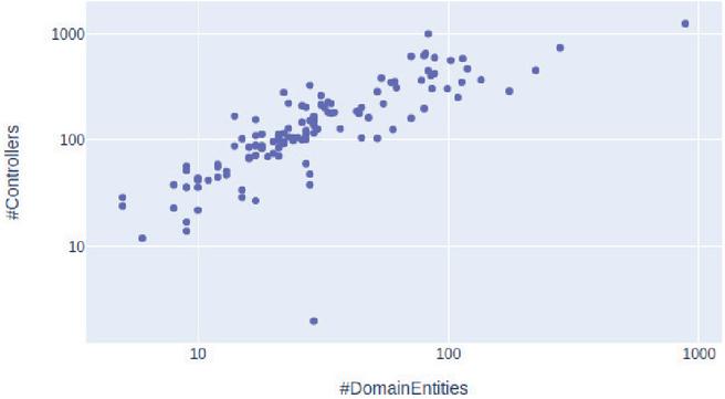
Figure 3 Representation of the 121 systems used in the evaluation.

The average number of lines of code considering all the codebases was $43468$ , with a standard deviation of $70286$ . This shows that we considered significantly different codebases, while in the literature it is frequent the use of toy or small systems, e.g., [16, 32].

To identify which combination of similarity measures provides better decompositions in terms of complexity, coupling and cohesion, we performed an extensive analysis with the data collected from the 121 monolith systems.

For each codebase, we used our tools to generate several dendrograms, by varying the weights of the four existing similarity measures, in intervals of 10 in a scale of 0 to 100, and then performed several cuts on each one. Each cut resulted in a candidate decomposition of the monolith with a specific number of clusters, varying from 3 to 10. Note that, depending on the number of domain entities, the number of clusters were proportional to the number of entities of the system. For instance, if a monolith has between 10 to 20 domain entities only three decompositions are considered, with 3, 4 and 5 clusters. Then, the values for the 3 metrics were calculated for each generated decomposition.

Since the values of the complexity metric depend on the number of functionalities in each monolith, in order to compare them among the different monoliths, it was necessary to uniform the complexity values:

U n i f o r m C o m p l e x i t y (d, s) = \frac{c o m p l e x i t y (d)}{m a x C o m p l e x i t y (s)}

Where the uniform complexity of a given decomposition $d$ of a monolith is calculated by dividing the complexity of $d$ by the $m a x C o m p l e x i t y$ . The $m a x C o m p l e x i t y$ value is determined by calculating the complexity of a decomposition of the monolith where each cluster has a single domain entity. Therefore, the uniform complexity of any monolith decomposition is a value in the interval 0 to 1.

5.2 Metrics Evaluation

As cohesion and coupling metrics are used to assess the quality of monolith decompositions, we want to study whether the decompositions that minimize the transactional complexity also tend to provide good results in terms of modularity.

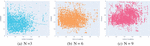
After generating, for each system, the decompositions for the different values of N resulting from all the combinations of similarity measures, we calculate the graphs in Figure 4, where each marker represents a decomposition of a specific monolith system, obtained from a specific combination of similarity measures. A regression line representing the correlation between the complexity (uniform complexity) and coupling values is also represented.

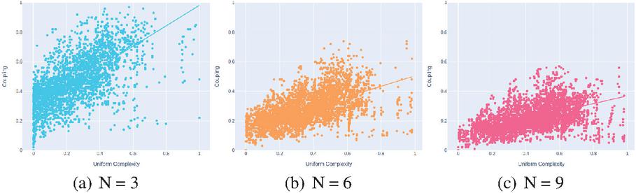
Figure 4 Analysis of the correlation between the complexity and coupling metrics for decompositions with different N values, resulting from all the combination of similarity measures, considering the data collected from the selected 121 systems.

All graphs seem to show a positive correlation between complexity and coupling. We can observe that the regression lines always have a positive slope, and that it tends to become less positive as the N is increased. Furthermore, we can observe that as the value of N increases, the constant values of the regression lines tend to decrease, indicating that decompositions with more clusters tend to have lower coupling. The Coefficient of Determination ( $R^{2}$ ) values obtained for each graph are 0.38, 0.34 and 0.29 for N = 3, 6, and 9, which are significantly higher in comparison to the cohesion evaluation and can potentially suggest a good correlation between the variables.

To confirm this, we validated the following regression model that relates the coupling of a decomposition $d$ with its complexity and number of clusters, using the Ordinary Least Squares (OLS) method:

C o u p l i n g (d) = β_{1} \cdot U n i f o r m C o m p l e x i t y (d) + β_{2} \cdot # d . c l u s t e r s + c o n s

The OLS regression results allowed us to reject the null hypothesis at a 0.05 significance level and state with 95% confidence that there is a statistically significant relationship between coupling and both the number of clusters and complexity. The number of clusters has a negative coefficient while the uniform complexity has a positive coefficient. This indicates that, based on our data-set, among decompositions with similar complexity, the ones with more clusters tend to be, on average, less coupled, and among decompositions with the same number of clusters, the ones with more complexity tend to be, on average, more coupled. Considering that complexity varies between 0 and 1, we consider that the uniform complexity coefficient of 0.4 is very significant. This was expected because decompositions with high complexity usually result from having functionalities composed of a higher number of local transactions, on average, which leads to more interactions between clusters, tending to increase the coupling between pairs of clusters, and therefore, the coupling of the overall decomposition.

A slightly negative coefficient ( $-$ 0.04) for the number of clusters coefficient means that by introducing a new cluster, the average dependencies between each pair of clusters tends to decrease. This result may seem a bit odd, since the increment of the number of clusters intuitively suggests more communication between clusters, however, note that this does not mean that the total number of dependencies between clusters decreases with a new cluster. It means that, on average, the number of dependencies that are introduced in the new partition is small in comparison to the weight of introducing a new cluster in the measure of the coupling of the whole system (that is determined by calculating the average of cluster’s coupling).

Finally, the $R^{2}$ value obtained for this regression model was 0.44, which shows a stronger correlation between coupling and both complexity and number of clusters, and allows us to conclude that decompositions with higher complexity tend to have worse (higher) values in terms of the coupling quality and support the conclusion made in the previous work.

A similar analysis was done for the correlation between complexity and cohesion metrics. In Figure 5, each marker represents a decomposition of a specific monolith system, obtained from a specific combination of similarity measures. A regression line represents the correlation between the complexity (uniform complexity) and cohesion values.

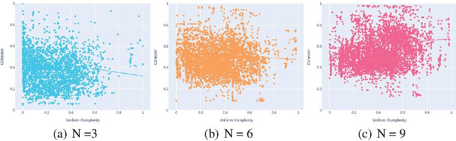
Figure 5 Analysis of the correlation between the complexity and cohesion metrics for decompositions with different N values, resulting from all the combination of similarity measures, considering the data collected from the selected 121 systems.

The graphs don’t seem to show a correlation between complexity and cohesion. For most of the N values the regression line tends to have a slightly negative slope, indicating that higher complexity values tend to be associated with lower cohesion values, however, as the N increases the slope becomes less negative and for N $=$ 9 the slope even becomes positive. The coefficient of determination ( $R^{2}$ ) values obtained for each graph are very low as well: 0.022, 0.007 and 0.014 for N $=$ 3, 6, and 9, respectively, which means that there is a high variability within our data-set. Furthermore, we can observe that as the value of N increases, the overall cohesion of the decompositions tends to increase as well, indicating that decompositions with more clusters tend to have higher cohesion.

From analysis done using the regression model the value obtained for $R^{2}$ is 0.110, which is considerably low. This means that, although there is a statistically significant relationship between the variables, only 11% of the variation in the cohesion of the decompositions may be explained by its number of clusters and complexity.

5.3 Similarity Measures Evaluation

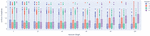
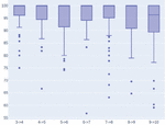
Figure 6 represents the uniform complexities of all the generated decompositions with 3 clusters, where each marker represents a decomposition obtained from a combination of similarity measures where a similarity measure’s value (denoted by the color) has a fixed weight percentage ( $x$ axis), and the remaining percentages vary across the other measures.

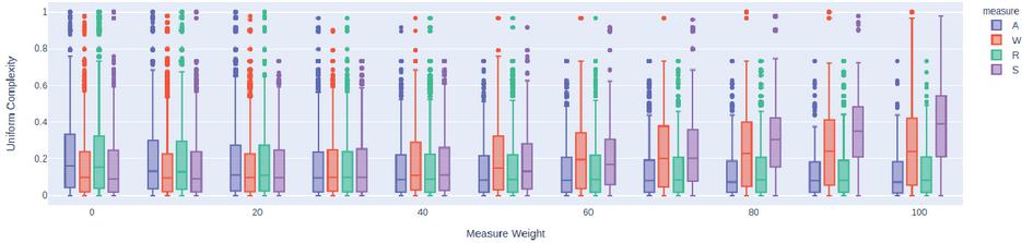
Figure 6 Decompositions’ complexities when the weight of each measure (A $=$ Access, W $=$ Write, R $=$ Read, S $=$ Sequence) is fixed at a specific value while the remaining vary. The markers represent all the generated decompositions with 3 clusters considering all the codebases.

We can observe, from the size and height of the boxes, that for 3 clusters, as more weight is given to the access and read similarity measures the complexity tend to decrease, while the opposite occurs for the write and sequence similarity measures. Furthermore, we could also observe in other graphs (not represented), that when the number of clusters increases the complexity also tends to increase, regardless of the measure used. For these cases

1. the discrepancy between the performances of the similarity measures becomes almost unnoticeable and

2. all the similarity measures generate decompositions with both high and low complexities.

To confirm this, we validated the following linear regression that assesses the correlation of the complexity of a decomposition with the weights given to each similarity measure and its number of clusters, using the Ordinary Least Squares method:

$u C o m p l e x i t y (d)$	$= β_{1} \cdot d . w e i g h t_{A} + β_{2} \cdot d . w e i g h t_{W}$
	$+ β_{3} \cdot d . w e i g h t_{R} + β_{4} \cdot d . w e i g h t_{S}$
	$+ β_{5} \cdot # d . c l u s t e r s + c o n s$

To test this regression, we defined the following hypotheses:

• $H_{0}$ : $β_{1} = β_{2} = β_{3} = β_{4} = β_{5} = 0$ ; meaning that the complexity of a decomposition does not have a relation with any of the five parameters

• $H_{1}$ : $β_{1} \neq 0 \lor β_{2} \neq 0 \lor β_{3} \neq 0 \lor β_{4} \neq 0 \lor β_{5} \neq 0$ ; meaning that the complexity of a decomposition does have a relation with at least one of the five parameters

The regression results obtained allow us to reject the null hypothesis at a significance level of 0.05. It also allows to conclude that the coefficients for the number of clusters (0.0353), read (0.0001), the write (0.0014), and sequence (0.0014) similarity measures have a statistically significant positive correlation with complexity. For the access measure we can’t conclude neither a negative nor a positive correlation since it has a coefficient of $-$ 1.721e-06 with its confidence interval between [ $-$ 3.65e-05, 3.31e-05], which is a very positive result, since it suggests that using higher weights on this measure can stagnate, or, ultimately, decrease the complexity of the generated decompositions.

The positive coefficient on the number of clusters is expected, since with the increment of the number of clusters, some functionalities are split into more clusters, increasing the number of local transactions per functionality and the overall decomposition’s complexity.

The obtained $R^{2}$ value for this regression model was 0.193, which is considerably low. This means that there is a significant variability within our data-set and that, although some measures achieved lower coefficients than others, it’s hard to conclude that one single similarity measure can provide better results than another in terms of complexity.

Concerning the impact of the combination of the similarity measures on the cohesion metric, we did a similar analysis. The regression results for this evaluation showed that the access, read, write and sequence measures have a statistically significant positive correlation with cohesion with coefficients of 0.0043, 0.0043, 0.0035, and 0.0036, respectively, as well as the number of clusters with a coefficient of 0.0243. However, the value of $R^{2}$ is still very low, 0.123, and so, although the access and read measures show better coefficients, it doesn’t allow us to take conclusions about the performance of the similarity measures regarding cohesion.

Similarly, we did an evaluation to assess the correlation between the decomposition measure’s weights and number of clusters with coupling. The regression results for this evaluation showed that the access, read, write and sequence weights have a statistically significant positive correlation with coupling with coefficients of 0.0040, 0.0041, 0.0052 and 0.0050, respectively, while the number of clusters has a statistically significant negative correlation with coupling with a coefficient of $- 0.0290$ . Once again, although the coefficients are aligned with the previous results, with the access and read measures showing better coefficients, the value of $R^{2}$ is still low, 0.227, hence, we can’t conclude that the used combination of similarity measures is enough to explain a decomposition’s coupling.

Summarizing these results, although, on average, the higher weights on the access and read similarity measures tend to provide better decompositions regarding the three quality metrics, we conclude that the measures combinations by themselves cannot predict the quality of a monolith’s decomposition and that in order to achieve better correlations new variables, related with other monolith’s characteristics, should be included in the evaluations.

5.4 Detailed Analysis

In order gain further insights into what is the impact of the similarity measures on the complexity of the decompositions, we have done a more detailed data analysis.

5.4.1 Write Similarity Measure

The conclusion that the use of higher weights in the sequence measure tends to provide the highest complexities is expected, since the rationale behind this measure often enables cases where the coupling between entities is not perceived, e.g., when two entities are never seen consecutively although they share exactly the same controllers. However, it is not clear why the write similarity measure has the same performance, raising the question of why the write measure doesn’t provide similar results to the access and read measures.

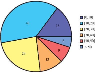
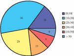
Figure 7 Number of codebases whose percentage of write accesses is within the respective interval, considering all the identified accesses.

Figure 7 shows that, for most of the analysed codebases, the percentage of write accesses identified is below 30%. This suggests that there aren’t many controllers that perform writes, hampering the identification of similarity between pairs of entities when using this measure. This can be the answer to our question and indicates that to choose what is the adequate similarity measure combination to apply it may be worth characterize first the codebase, for example, in terms of percentage of reads and writes.

Therefore, we evaluated the relation between the percentage of write accesses in a monolith and the performance of the write similarity measure when decomposing the same monolith. To assess this relation, we first identified the write measure’s performance for each monolith system. We considered a system’s write similarity measure’s performance as the coefficient obtained for the write measure when calculating a regression model that only includes the decompositions of the respective system.

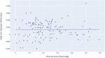
Figure 8 represents the correlation between the percentage of monolith’s write accesses ( $x$ axis) with the performance of the write similarity measure ( $y$ axis), where each marker represents a monolith system.

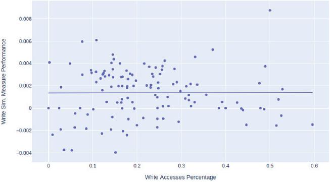
Figure 8 Correlation between the percentage of monolith’s write accesses and the performance of the write similarity measure.

The coefficient obtained for this linear regression was $5.796 e - 05$ , which is very close to zero, and the $R^{2}$ value obtained was $\sim 0.000$ , which is extremely low. This suggests that the percentage of write accesses by itself can’t explain the performance of the write similarity measure, i.e., there isn’t any relation between them. Since we only used one independent variable, we’re most likely facing the Omitted Variable Bias problem, i.e., leaving relevant variables out of our statistical model that could better explain the performance of this similarity measure. This leads us to conclude that, we should find other variables that could better explain this model in order to understand in which cases this measure could be more useful.

However, we noticed that there are some monolith systems that, even with low percentage of write accesses, can achieve low complexity decompositions when using higher weights on the write similarity measure.

One of the monoliths in which the write similarity measure had a good performance was SpringBlog.¹⁴ When experimenting various combinations of similarity measures to decompose SpringBlog into a 3 clusters system, we noticed that the decompositions with lower complexity were the ones obtained from combinations with high weights on the write similarity measure. We observed that in these decompositions the written domain entities are accessed by non-distributed functionalities, which, therefore, have no redesign cost. This shows that, although the write similarity measure slightly under-performed comparing to the access and read measures there are cases where in order to find the decompositions that guide towards the lowest complexity values, higher weights have to be given to it.

5.4.2 Discard write and sequence measures?

Therefore, the next research question to know whether it is possible to discard the write and sequence similarity measures when searching for the lowest complexity’s decomposition of a monolith?

We already saw an example where the write similarity measure would achieve a better decomposition comparing to the read measure, however, that could be uncommon enough not to justify the existence of this measure. To evaluate this hypothesis, we assessed the lowest and the highest complexity decompositions for each monolith system and different values of N.

To do that, for each N value, we selected the lowest and the highest complexity decompositions of each monolith system and calculated an average between the respective combinations of similarity measures that lead towards that decomposition. We considered the average between different combinations of similarity measures as the average between the weights of each measure. For example, the average between the combinations [10,20,30,40] and [20,30,50,0] would be [15,25,40,20]. Note that, for the same system, it is possible to have more than one combination of similarity measures generating dendrograms that lead to decompositions with identical complexity for the same number of clusters, which means that it is possible to have more than one best/worst solution (in terms of complexity). For these cases, we considered the best/worst combinations as the average between all the different combinations that provided the lowest/highest complexity decompositions.

The results obtained regarding the average combination weights that lead to the lowest and highest complexity decompositions for different values of N, together with the standard deviation, considering the 121 codebases, are represented in Tables 1 and 2, respectively.

Table 1 Average combination of similarity measure weights that lead to the decompositions with lowest complexity

			Weights
			A	W	R	S
N	3	avg	28.19	23.7	27.45	20.66
		std	26.13	27.39	26.88	19.78
	4	avg	33.42	21.56	23.66	21.36
		std	27.0	20.78	24.5	20.35
	5	avg	29.39	18.52	31.02	21.07
		std	27.75	21.9	30.58	22.37
	6	avg	26.44	22.54	27.19	23.83
		std	25.2	23.41	27.63	23.97
	7	avg	26.8	24.88	25.21	23.11
		std	25.52	26.07	23.93	24.69
	8	avg	34.64	19.64	25.22	20.49
		std	29.1	25.91	23.95	25.74
	9	avg	29.98	21.01	27.5	21.52
		std	30.29	23.99	26.48	24.11
	10	avg	26.42	19.25	26.0	28.33
		std	23.15	18.82	24.67	25.94

When looking at the results regarding the lowest complexity decompositions (Table 1), we can observe that, regardless of the N value:

• the average weights obtained for the access similarity measure are most of the times the highest (6/8 times) or the second highest (2/8 times);

• the average weights obtained for the write similarity measure are always either the lowest (5/8 times) or the second lowest (3/8);

• the average weights obtained for the read similarity measure are most of the times the second highest (6/8 times) or the highest (2/8 times);

• the average weights obtained for the sequence similarity measure are always either the lowest (3/8 times) or the second lowest (5/8).

These observations are aligned with the coefficient values previously obtained in the OLS regression model. Although the highest/lowest averaged measures tend to be consistent, with the access and read measures averages being always higher than the write and sequence ones, we don’t see a high variation among their values. All the averaged weights are within the interval starting in $18.52$ and ending in $34.64$ . Furthermore, the standard deviation values obtained for each similarity measure’s average are roughly as high as the average itself, for all the N values. This allows us to conclude that:

• There isn’t any particular combination of similarity measures that always provides the lowest complexity decompositions, because the standard deviations achieved were very high for all the measures;

• On average, the combinations the lead towards the lowest complexity decompositions tend to have the weights fairly well-distributed among the different measures, because the averages obtained are all contained within a small weight percentage interval.

Table 2 Average combination of similarity measure weights that lead to the decompositions with highest complexity

			Weights
			A	W	R	S
N	3	avg	5.17	18.9	4.2	71.73
		std	15.15	26.57	11.23	32.68
	4	avg	4.52	23.0	7.64	64.83
		std	12.55	33.4	18.58	39.73
	5	avg	7.48	22.72	7.8	62.0
		std	18.14	31.19	17.15	39.91
	6	avg	8.09	17.62	5.3	68.99
		std	20.51	26.01	11.0	35.05
	7	avg	9.82	19.64	10.1	60.44
		std	20.19	29.32	21.4	40.16
	8	avg	6.7	22.67	9.68	60.95
		std	15.04	30.76	19.57	38.1
	9	avg	11.82	23.01	9.78	55.39
		std	25.51	30.52	16.91	39.82
	10	avg	7.51	25.68	13.74	53.07
		std	17.45	30.58	24.21	38.8

When we look at the results regarding the highest complexity decompositions the results are more distinct.

There is an obvious constantly higher value on the calculated averages for the sequence similarity measure, and considering its high value, the standard error is not high enough to make us believe that cases where its weight is low when facing the worst decompositions will often happen. On the other hand, we can see a constantly low value for the calculated averages for the access and read similarity measures with low standard errors. The calculated averages for the write similarity measure is consistently higher than the access and read’s averages and lower than the sequence’s averages, for the several N values, and has medium-high standard errors, which means that it can either have a high and low weight percentages when considering the worst decompositions.

From these observations we conclude that:

• The combination of similarity measures that lead towards the worst decompositions in terms of complexity tend to have high weight percentages on the sequence measure;

• The worst decompositions in terms of complexity tend to result from a combination of measures where the weight percentage on the write measure is higher than the weight percentage on the access and read measures.

Based on this analysis, we conclude that, although we can make an association between the worst decompositions and the distribution of weights across the different similarity measures, all the measures showed to be equally indispensable in order to achieve the best decompositions in terms of complexity, hence, none of the measures should be discarded.

5.4.3 Access Measure Only?

We’ve seen that the best decompositions in terms of complexity are usually achieved using a combination that takes all the similarity measures into account. Nevertheless, from the previous evaluations, we also saw that the access similarity measure consistently showed slightly better performance indicators. Taking this into account, we raise the question: can we achieve decompositions close to the best solution by using solely the access similarity measure?

To answer this question we calculate:

D i s t a n c e_{100 A c c e s s e s} (m, N)

= \frac{Δ (100 A c c e s s C o m p l e x i t y (m, N), L o w e s t C o m p l e x i t y (m, N))}{Δ (A v e r a g e C o m p l e x i t y (m, N), L o w e s t C o m p l e x i t y (m, N))}

It compares, for each monolith, $m$ , and different values of N, the distance between the following two values:

1. The distance between the complexity of the decomposition generated using 100% weight on the access similarity measure ( $100 A c c e s s C o m p l e x i t y (m, N)$ ) and the complexity of the lowest complexity’s decomposition ( $L o w e s t C o m p l e x i t y (s, N)$ );

2. The distance between the average of all the complexity values considering the decompositions resulting from all the possible combinations of similarity measures ( $A v e r a g e C o m p l e x i t y (m, N)$ ) and the complexity of the lowest complexity’s decomposition ( $L o w e s t C o m p l e x i t y (m, N)$ ).

A $D i s t a n c e_{100 A c c e s s e s}$ value close to 0 means that the complexity of the decomposition obtained using solely the access similarity measure is very close to the complexity of the lowest complexity decomposition. A $D i s t a n c e_{100 A c c e s s e s}$ value close to (or higher than) 1 means that the complexity of the decomposition obtained using solely the access similarity measure is identical to (or even higher than) the average among all the decomposition’s complexities. Note that the monoliths whose $m a x C o m p l e x i t y$ was 0 were not included in this evaluation, because the calculated $D i s t a n c e_{100 A c c e s s e s}$ values would always be 0, which wouldn’t add any useful information.

After calculating this metric for all the 121 codebases and different values of N, we calculated, for each N, the average and the standard error among all the $D i s t a n c e_{100 A c c e s s e s}$ values obtained. The results obtained are represented in Table 3.

Table 3 Average of the $D i s t a n c e_{100 A c c e s s e s}$ values obtained for all the 121 codebases for different N values

N	3	4	5	6	7	8	9	10
avg	0.76	0.69	0.9	0.77	0.82	0.91	0.86	0.95
se	2.02	0.87	1.1	0.7	0.73	0.87	0.89	0.83

From the obtained results, we can observe that the average $D i s t a n c e_{100 A c c e s s e s}$ values calculated vary between 0.69 and 0.95. This means that, on average, the decompositions that use this combination of similarity measures are slightly better in terms of complexity than the average decomposition, since the $a v g$ values never reached or surpassed 1, but are much closer to the average decomposition than to the best decomposition. However, if we look at the standard errors, they are very high for all the N values, which means that, some times, this combination of similarity measures can either lead to decompositions with complexity values very close to the complexity of the lowest complexity decomposition or significantly far from it, beyond the average decompositions’s complexity. The high standard error across all the N values suggest, once more, that characterizing a codebase based on other aspects could help us find the types of codebases where a combination identical to this one could achieve the best and the worst decompositions.

From this analysis, we conclude that, most of the times, relying solely on the access similarity measure won’t lead to the best decomposition of a monolith nor to a decomposition that is identical to it, therefore, it shouldn’t be used alone.

5.5 Incremental Migration

Microservices experts recommend an incremental migration strategy of the monolith to the microservices architecture [33, Chapter 13]. However, there is no evidence that the best decomposition for N+1 clusters is an incremental partition of the best decomposition with N clusters. To evaluate this incrementality, we assessed what is the minimum number of changes required in the best decomposition with N clusters, so that the lowest complexity decomposition with N+1 clusters can be incrementally obtained from it, with N varying from 3 to 9. To measure those changes we used the MoJoFM metric [38].

MoJoFM is a distance measure between two architectures expressed as a percentage. This measure is based on two key operations used to transform one decomposition into another: moves (Move) of entities between clusters, and merges (Join) of clusters. Given two decompositions, A and B, MoJoFM is defined as:

M o J o F M (A, B) = (1 - \frac{m n o (A, B)}{m a x (m n o (\forall A, B))}) \times 100 %

where $m n o (A, B)$ is the minimum number of Move and Join operations needed to transform A into B and $m a x (m n o (\forall A, B))$ is the number of Move and Join operations needed to transform the most distant decomposition from B into B. Therefore, MoJoFM quantifies the amount of effort required to transform one architecture into another. A 100% MoJoFM value indicates full correspondence between A and B, while a 0% MoJoFM value indicates that the two architectures are completely different.

The results obtained are represented in Figure 9, where each marker represents the calculated MoJoFM value for a $N \to N + 1$ transition of a specific codebase.

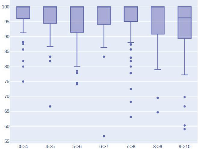
Figure 9 MoJoFM between the best decomposition with N clusters and the closest decomposition from which the best decomposition with N+1 clusters can be obtained incrementally, considering the 121 codebases’ decompositions.

We can observe that, except for the $9 \to 10$ transition, where the median has 96.3% MoJoFM, the median of each transition is equal to 100% MoJoFM. This means that, for at least nearly half of all the transitions tested, considering all the codebases, no additional changes are required at all. In fact, 59.3% of the transitions tested have a 100% MoJoFM value and 84.7% of the transitions tested have a MoJoFM greater or equal to 90%, which is a very positive result. We can also observe the existence of some outlier transitions. These transitions usually have a MoJoFM value lower than 80%, which represents only 4% of all the transitions tested. We noticed that the transitions with lower MoJoFM values usually are from codebases with lower number of entities, in which the move and join operations end up having more weight, since the farthest decomposition ( $m a x (m n o (\forall A, B))$ ), is less distant.

6 Related Work

In recent years, myriad of approaches to support the migration of monolith systems to microservices architectures have been proposed [1, 16, 17, 4, 22, 25, 13, 26, 9, 15, 35, 39], which use the monolith specification, codebase, services interfaces, run-time behavior, and project development data to recommend the best decompositions [31].

Our work approach addresses static analysis over monolith codebases. Some work, such as [20] and [37], despite not following the same collection approach, end up having similarities with our cluster generation methodology. Additionally, it is common to see the same three phases of our migration process across other research, however, there’s dissimilarity on what the main concern is, leading to the use of different similarity measures, such as accesses [20], reads [3, 37], writes [3, 37], and sequences [3, 8].

Some of these approaches also use different metrics to assess the result of their decompositions. Therefore, we studied the literature on microservices quality to identify which metrics to consider. The complexity metric we used for evaluating the complexity of the decompositions, defined in the previous work [34], is based on the current state of the art metrics for service-oriented systems [5]. Other complexity metrics use the percentage of services with support for transactions [18], but they lack an integrated perspective that we provide by associating the lack of isolation with the transactional complexity of a functionality in a microservices architecture. Other complexity metric consider the number of operations and services that can be executed in response to an incoming request [30, 2], while we consider the complexity of implementing a local transaction in the terms of inter-functionalities interactions, which emphasizes the complexity of cognitive load, i.e., the total number of other functionalities to consider when redesigning a functionality.

In what concerns the coupling and cohesion metrics, the definitions in the context of services consider, for the coupling metric, the number of operations in the service interfaces that are used by other services, where a higher number reflects a higher coupling, and, for the cohesion metric, the percentage of operations of the service interface that are used together [30]. These metrics based on the interface definition are defined in the assumption that it is necessary to measure the coupling and cohesion of systems of services without having access to the services implementation. In our case, since we are working on the migration of a monolith, we can define them in term of the domain entities that implement the services: coupling as the percentage of domain entities exposed in the interface, and cohesion as the percentage of the cluster domain entities that are used together to accomplish a functionality. This provides more precise results because the interface operations do not reveal what occurs inside the microservice.

7 Discussion

7.1 Lessons Learned

From this research we learned the following lessons:

• It is not possible to conclude that one of the similarity measures determines the generation of the best decomposition according to any of the three metrics;

• The combination of the similarity measure values for the best decomposition according to the quality metrics may be dependent on specific characteristics of the monolith system;

• The best approach is to run our analyser feature to find the best combination of similarity measures for each monolith;

• Our approach supports the incremental migration of a monolith to microservices.

7.2 Threats to Validity

7.2.1 Internal Validity

Some of the gathered codebases had few database accesses that weren’t implemented by Spring Data JPA repositories. For these cases, we manually replaced them with calls to new repository methods, implemented by ourselves, that accessed the same tables in the same mode, so that we could use the respective codebase without losing any information. It is possible that a call may have passed unnoticed or some type of mistake have been introduced, however, we took advantage of the Java IDE’s features to find and replace the respective accesses and we’re confident in discarding this as a threat.

The algorithm used to collect the accesses made during the execution of a functionality returns a chain of all the possible paths of its execution. For example, if we have a controller composed by an if/else branch, the list of accesses returned for this controller will be composed by the accesses made when the if branch is executed concatenated with the ones made when the else branch is executed. This means that our final list of accesses may contain pairs of accesses that cannot happen consecutively (the last access of the if branch and the first of the else branch). The sequence similarity measure calculates the distance between entities based on the consecutive accesses information, therefore, there is the possibility that the similarity matrices produced by this similarity measure are biased by some of these pairs of accesses that cannot happen. This may have a higher impact on the sequence similarity measure.

7.2.2 External Validity

To select the codebases used in the static analysis evaluation section we followed a systematic and automated approach. Nevertheless, there is the possibility that the selected codebases may have biased the gathered results. However, taking into account the high number of selected codebases and the variability among them, we are confident in discarding this as a threat to validity. Moreover, we are confident that the results can be generalized to monoliths implemented using the MVC architectural style, because the different technological frameworks follow similar solutions as Spring-Boot and Spring Data JPA. Actually, the best software architecture solutions for the development of MVC systems are copied (shared) by the different frameworks.

Due to the diversity of metrics that exist for complexity, coupling and cohesion, can our results be generalized? Despite this diversity, we are confident that the results are relevant because the several metrics analyse the same elements. Our complexity metric focus on the complexity introduced by transactions and the complexity of the interactions, like other metrics do. Concerning cohesion and coupling, our metrics measure how cluster domain entities are visible outside the cluster and how they are accessed together in the context of a functionality, which corresponds to the level of dependencies between clusters, how many domain entities are not encapsulated, and whether all the cluster domain entities contribute to the single responsibility principle. Anyway, as far as we know, there is not a standard metric for each of these qualities, and research must be done to compare their results, as it is reported elsewhere [2], which is outside the scope of our work.

7.3 Future Work

As a consequence of the results of this research and the learned lessons we identify the following topics for future work:

• Experiment with machine learning techniques using the metrics as fitness functions to infer which combination of similarity measures is more adequate for a concrete monolith system;

• Currently, the static collection of data captures a single trace for each functionality, but it is worth experimenting if the data collected using several traces, one for each independent path of execution, produces better decompositions;

• Further explore the results of the dynamic collection of data, in terms of the frequency of each of the functionalities, and define new similarity measures to verify if it can generate better decompositions.

8 Conclusions

The migration of monolith systems to the microservices architecture is a complex problem that software development teams have to address when systems become more complex and larger in scale. Therefore, it is necessary to develop the methods and tools that help and guide them on the migration process. One of the most challenging problems is the identification of microservices. Several approaches have been proposed to automate such identification, which, although sometimes similar, use different monolith analysis techniques, similarity measures, and metrics to evaluate the quality of the system.

In this paper, we leveraged previous work, extended its analysis capabilities and scope, and applied it on 121 codebases to further evaluate it. From the results of our study, we conclude that there is not a particular similarity measure that generates the best decompositions, considering the quality metrics for complexity, coupling and cohesion, and we raise the hypothesis that the best similarity measure may depend on particular characteristics of the monolith. Therefore, we suggest the use of the analyser feature that generates decompositions using an extensive combination of similarity measures to find the one that has the best quality.

Additionally, we verified that our solution supports an incremental migration process of a monolith, because the best proposed decomposition with N+1 clusters can, most of the times, be obtained by further decomposing the best proposed decomposition with N clusters, which is a good result, since this is the recommended migration strategy by microservices experts.

As an additional contribution, the tool’s code and collected data is publicly available in a GitHub repository so that third parties can do further research. The data collection tool is in,¹⁵ the collected data from the codebases is in,¹⁶ and the scripts used in the analysis in.¹⁷

Acknowledgements

This work was supported by national funds through FCT, Fundação para a Ciência e a Tecnologia, under project UIDB/50021/2020.

Footnotes

¹ https://docs.scipy.org/doc/

² https://spring.io/projects/spring-boot

³ https://fenix-framework.github.io/

⁴ http://www.hibernate.org/

⁵ https://www.eclipse.org/eclipselink/

⁶ http://openjpa.apache.org/

⁷ https://docs.spring.io/spring-data/jpa/docs/current/reference/html/

⁸ https://docs.jboss.org/hibernate/core/3.3/reference/en/html/queryhql.html

⁹ http://spoon.gforge.inria.fr/mvnsites/spoon-core/apidocs/spoon/reflect/visitor/CtScanner.html

¹⁰ https://github.com/JSQLParser/JSqlParser

¹¹ https://docs.jboss.org/hibernate/orm/4.3/javadocs/org/hibernate/hql/internal/ast/HqlParser.html

¹² https://jsoup.org/

¹³ https://github.com/spring-projects/spring-data-jpa/network/dependents

¹⁴ https://github.com/bvn13/SpringBlog

¹⁵ https://github.com/socialsoftware/mono2micro/tree/master/collectors/spoon-callgraph

¹⁶ https://github.com/socialsoftware/mono2micro/tree/master/data/static

¹⁷ https://github.com/socialsoftware/mono2micro/tree/master/backend/src/main/resources/evaluation

References

[1] M. Ahmadvand and A. Ibrahim. Requirements reconciliation for scalable and secure microservice (de)composition. In 2016 IEEE 24th International Requirements Engineering Conference Workshops (REW), pages 68–73, Sep. 2016.

[2] O. Al-Debagy and P. Martinek. A metrics framework for evaluating microservices architecture designs. Journal of Web Engineering, 19(3–4):341–370, 2020.

[3] M. J. Amiri. Object-aware identification of microservices. In 2018 IEEE International Conference on Services Computing (SCC), pages 253–256, 2018.

[4] Luciano Baresi, Martin Garriga, and Alan De Renzis. Microservices identification through interface analysis. In Flavio De Paoli, Stefan Schulte, and Einar Broch Johnsen, editors, Service-Oriented and Cloud Computing, pages 19–33, Cham, 2017. Springer International Publishing.

[5] Justus Bogner, Stefan Wagner, and Alfred Zimmermann. Automatically measuring the maintainability of service- and microservice-based systems: A literature review. In Proceedings of the 27th International Workshop on Software Measurement and 12th International Conference on Software Process and Product Measurement, IWSM Mensura ’17, page 107–115, New York, NY, USA, 2017. Association for Computing Machinery.

[6] João Cachopo and António Rito-Silva. Combining software transactional memory with a domain modeling language to simplify web application development. In Proceedings of the 6th International Conference on Web Engineering, ICWE ’06, page 297–304, New York, NY, USA, 2006. Association for Computing Machinery.

[7] Andrés Carrasco, Brent van Bladel, and Serge Demeyer. Migrating towards microservices: Migration and architecture smells. In Proceedings of the 2nd International Workshop on Refactoring, IWoR 2018, page 1–6, New York, NY, USA, 2018. Association for Computing Machinery.

[8] Mohamed Daoud, Asmae El Mezouari, Noura Faci, Djamal Benslimane, Zakaria Maamar, and Aziz El Fazziki. Automatic microservices identification from a set of business processes. In Mohamed Hamlich, Ladjel Bellatreche, Anirban Mondal, and Carlos Ordonez, editors, Smart Applications and Data Analysis, pages 299–315, Cham, 2020. Springer International Publishing.

[9] L. De Lauretis. From monolithic architecture to microservices architecture. In 2019 IEEE International Symposium on Software Reliability Engineering Workshops (ISSREW), pages 93–96, 2019.

[10] N. Ford, R. Parsons, and P. Kua. Building Evolutionary Architectures. O’Reilly, 1 edition, 10 2017.

[11] Martin Fowler and James Lewis. Microservices a definition of this new architectural term. URL: http://martinfowler.com/articles/microservices.html, page 22, 2014.

[12] Armando Fox and Eric A. Brewer. Harvest, yield, and scalable tolerant systems. In Proceedings of the The Seventh Workshop on Hot Topics in Operating Systems, HOTOS ’99, page 174, USA, 1999. IEEE Computer Society.

[13] Jonas Fritzsch, Justus Bogner, Alfred Zimmermann, and Stefan Wagner. From monolith to microservices: A classification of refactoring approaches. In Jean-Michel Bruel, Manuel Mazzara, and Bertrand Meyer, editors, Software Engineering Aspects of Continuous Development and New Paradigms of Software Production and Deployment, pages 128–141, Cham, 2019. Springer International Publishing.

[14] Hector Garcia-Molina and Kenneth Salem. Sagas. SIGMOD Rec., 16(3):249–259, December 1987.

[15] M. H. Gomes Barbosa and P. H. M. Maia. Towards identifying microservice candidates from business rules implemented in stored procedures. In 2020 IEEE International Conference on Software Architecture Companion (ICSA-C), pages 41–48, 2020.

[16] Michael Gysel, Lukas Kölbener, Wolfgang Giersche, and Olaf Zimmermann. Service cutter: A systematic approach to service decomposition. In Marco Aiello, Einar Broch Johnsen, Schahram Dustdar, and Ilche Georgievski, editors, Service-Oriented and Cloud Computing, pages 185–200, Cham, 2016. Springer International Publishing.

[17] S. Hassan and R. Bahsoon. Microservices and their design trade-offs: A self-adaptive roadmap. In 2016 IEEE International Conference on Services Computing (SCC), pages 813–818, June 2016.

[18] Mamoun Hirzalla, Jane Cleland-Huang, and Ali Arsanjani. A metrics suite for evaluating flexibility and complexity in service oriented architectures. In George Feuerlicht and Winfried Lamersdorf, editors, Service-Oriented Computing – ICSOC 2008 Workshops, pages 41–52, Berlin, Heidelberg, 2009. Springer Berlin Heidelberg.

[19] W. Jin, T. Liu, Y. Cai, R. Kazman, R. Mo, and Q. Zheng. Service candidate identification from monolithic systems based on execution traces. IEEE Transactions on Software Engineering, pages 1–1, 2019.

[20] Wuxia Jin, Ting Liu, Yuanfang Cai, Rick Kazman, Ran Mo, and Qinghua Zheng. Service candidate identification from monolithic systems based on execution traces. IEEE Transactions on Software Engineering, 2019.

[21] Mike Keith and Merrick Schincariol. Pro EJB 3: Java Persistence API. Apress, 2006.

[22] S. Klock, J. M. E. M. V. D. Werf, J. P. Guelen, and S. Jansen. Workload-based clustering of coherent feature sets in microservice architectures. In 2017 IEEE International Conference on Software Architecture (ICSA), pages 11–20, April 2017.

[23] Glenn E. Krasner and Stephen T. Pope. A cookbook for using the model-view controller user interface paradigm in smalltalk-80. J. Object Oriented Program., 1(3):26–49, August 1988.

[24] Philippe Lalanda. Shared repository pattern. In Proc. 5th Annual Conference on the Pattern Languages of Programs. Citeseer, 1998.

[25] Genc Mazlami, Jürgen Cito, and Philipp Leitner. Extraction of microservices from monolithic software architectures. In Web Services (ICWS), 2017 IEEE International Conference on, pages 524–531. IEEE, 2017.

[26] R. Nakazawa, T. Ueda, M. Enoki, and H. Horii. Visualization tool for designing microservices with the monolith-first approach. In 2018 IEEE Working Conference on Software Visualization (VISSOFT), pages 32–42, Sep. 2018.

[27] Luís Fernando Ambrósio Nunes, Nuno Alexandre Vieira Santos, and António Rito Silva. From a monolith to a microservices architecture: An approach based on transactional contexts. In European Conference on Software Architecture (ECSA), volume 11681 of LNCS, pages 37–52. Springer International Publishing, September 2019.

[28] Charlene O’Hanlon. A conversation with werner vogels. Queue, 4(4):14–22, May 2006.

[29] Renaud Pawlak, Martin Monperrus, Nicolas Petitprez, Carlos Noguera, and Lionel Seinturier. Spoon: A library for implementing analyses and transformations of Java source code. Software: Practice and Experience, 46(9):1155–1179, 2016.

[30] M. Perepletchikov, C. Ryan, K. Frampton, and Z. Tari. Coupling metrics for predicting maintainability in service-oriented designs. In 2007 Australian Software Engineering Conference (ASWEC’07), pages 329–340, 2007.

[31] F. Ponce, G. Márquez, and H. Astudillo. Migrating from monolithic architecture to microservices: A rapid review. In 2019 38th International Conference of the Chilean Computer Science Society (SCCC), pages 1–7, 2019.

[32] Zhongshan Ren, Wei Wang, Guoquan Wu, Chushu Gao, Wei Chen, Jun Wei, and Tao Huang. Migrating web applications from monolithic structure to microservices architecture. In Proceedings of the Tenth Asia-Pacific Symposium on Internetware, Internetware ’18, New York, NY, USA, 2018. Association for Computing Machinery.

[33] Chris Richardson. Microservices patterns with examples in java. URL: https://www.manning.com/books/microservices-patterns, 2018.

[34] Nuno Santos and António Rito Silva. A complexity metric for microservices architecture migration. In 2020 IEEE International Conference on Software Architecture (ICSA), pages 169–178. IEEE, 2020.

[35] A. Selmadji, A. Seriai, H. L. Bouziane, R. Oumarou Mahamane, P. Zaragoza, and C. Dony. From monolithic architecture style to microservice one based on a semi-automatic approach. In 2020 IEEE International Conference on Software Architecture (ICSA), pages 157–168, 2020.

[36] D. Taibi and V. Lenarduzzi. On the definition of microservice bad smells. IEEE Software, 35(3):56–62, 2018.

[37] Shmuel Tyszberowicz, Robert Heinrich, Bo Liu, and Zhiming Liu. Identifying microservices using functional decomposition. In Xinyu Feng, Markus Müller-Olm, and Zijiang Yang, editors, Dependable Software Engineering. Theories, Tools, and Applications, pages 50–65, Cham, 2018. Springer International Publishing.

[38] Zhihua Wen and Vassilios Tzerpos. An effectiveness measure for software clustering algorithms. In Proceedings. 12th IEEE International Workshop on Program Comprehension, 2004., pages 194–203. IEEE, 2004.

[39] Y. Zhang, B. Liu, L. Dai, K. Chen, and X. Cao. Automated microservice identification in legacy systems with functional and non-functional metrics. In 2020 IEEE International Conference on Software Architecture (ICSA), pages 135–145, 2020.

Biographies

Samuel Santos has a M.Sc. from Instituto Superior Técnico (IST) of the University of Lisbon (UL).

António Rito Silva is an Associate Professor at Instituto Superior Técnico (IST) of the University of Lisbon (UTL) and researcher of Distributed Parallel and Secure Systems of INESC-ID. He received a PhD on software engineering in 1999 from the IST. His research interests include software architectures for microservices, digital humanities, and business process management (BPM). António has published more than 90 peer-reviewed articles in journals, conferences and workshops. He is leading research on the migration of monolith applications to a microservices architecture (https://github.com/socialsoftware/mono2micro).