Semantic Relation Extraction from Cultural Heritage Archives

Watchira Buranasing^{1, 2,}* and Woraphon Lilakiataskun¹

¹Faculty of Information Sciences and Technology, Mahanakorn university of technology, Nongchok, Bangkok, 10530, Thailand
²National Electronics and Computer Technology Center, Khlong Luang District, Pathumthani 12120, Thailand
E-mail: watchira.buranasing@nectec.or.th
*Corresponding Author

Received 17 October 2021; Accepted 05 February 2022; Publication 12 April 2022

Abstract

Digital preservation technologies are now being increasingly adopted by cultural heritage organizations. This cultural heritage data is often disseminated in the form of digital text through a variety of channels such as Wikipedia, cultural heritage archives, etc. To acquire knowledge from digital data, the extraction technique becomes an important part. However, in the case of digital text, which has characteristics such as ambiguity, complex grammar structures such as the Thai language, and others, it makes it more challenging to extract information with a high level of accuracy. We thus propose a method for improving the performance of data extraction techniques based on word features, multiple instance learning, and unseen word mapping. Word features are used to improve the quality of word definition by concatenating parts of speech (POS) and word position is used to establish the accurate definition of a word and convert all of this into a vector. In addition, we use multiple instance learning to solve issues where words do not fully express the meaning of the triple. We also cluster the particular word to find the predicate word by removing words that are irrelevant between the subject and the object. The difficulty of having a new set of words that have never been trained before can be overcome by using unseen word mapping with sub-word and nearest neighbor word mapping. We conducted several experiments on a cultural heritage knowledge graph to show the efficacy of the proposed method. The results demonstrated that our proposed technique outperforms existing models currently utilized in relation to extraction systems. It can achieve excellent accuracy since its precision, recall, and F1 score are 0.89, 0.88, and 0.89, respectively. Furthermore, it also performed well in terms of unseen word prediction, precision, recall, and F1 score, which were 0.81, 0.87, and 0.84, respectively.

Keywords: Digital archive, relation extraction, cultural archive, word vector representation, information extraction.

1 Introduction

Cultural heritage [1] represents the identity of culture as a way of life created by a group and passed from one generation to the next. In the age of digital information, cultural institutions are increasingly focusing on data collection in digital formats. Digital cultural information is beneficial not only for conservation, but also for education, tourism, innovation, and the creative economy. This has an impact on the city’s citizens’ social, cultural, and economic well-being. However, retrieving information from digital data has remained difficult, because each source serves a different purpose. As a consequence, the architecture of data structures varies, and some of them contain data in an unstructured format. The relation extraction technique [2] provides for the efficient access of important information when dealing with unstructured data and a variety of data formats. Previous studies [3] on relation extraction depended on pattern-matching rules that were manually developed for each domain to capture the relationship, such as the relationship between “location” and “city,” “author” and “book,” “festival” and “season”. These methods were effective in defined domains but not in general domains, and they also needed extensive specialist knowledge and human labour. While neural networks are an algorithm used in machine learning and used for relation extraction, one of the approaches utilized is to convert data into vector form to apply to discovering grammatically and semantically similar sets of terms. However, there is still a difficulty with using the word embedding basis alone to discover the relationship in the triple format when there is a new word. As a result, performance will be decreased.

To address this issue, we propose an alternative technique for improving the performance of relation extraction systems by focusing on phrase syntax and semantics. The inputs of this technique are word tokens, including word features as part of speech (POS) tagging and word position to improve the correctness of word definition for determining the correct definition of a word. We concatenate them and transform them into a low-dimensional vector for word embedding. We used multiple instance learning (MIL) to deal with issues such as words that did not express a relationship or meaning words that did not appear in the triple. We predicted the relationship from the unseen word pair by mapping the unseen words to trained embedding without redoing training, which reduces a lot of time and resources. We performed various experiments on a cultural heritage knowledge graph to demonstrate the effectiveness of the proposed method.

The remainder of this paper is organized as follows: The second section provides an overview of related works. Section three provides an overview of the approach, while Section four shows the findings of the experiments. Section five presents conclusions and suggests future research directions.

2 Related Work

One of the most popular techniques for relation extraction systems is using machine learning algorithms such neural networks. Thien Huu Nguyen and Ralph Grishman [4] used CNN as their relation extraction model, as well as supervised natural language processing (NLP). This approach utilizes window sizes as filters, and also position embeddings to detect relationship distancing. However, utilizing simply the position feature for relation extraction cannot detect the entity’s predicate. For relation extraction and named entity recognition, Daniel Khashabi [5] used recursive neural networks (RNNs) without external feature designs. The complicated context may not be extracted by this model.

Word vector representation techniques have become the most preferred approach in recent years. These techniques are used by Global Vectors (GloVe) [6] and Word2vec [7] to increase the performance of relation extraction models. GloVe is a method for creating word embeddings that is based on matrix factorization techniques on a word-context matrix. Word2vec expresses words in a two-dimensional space, with each dimension representing a different syntactic or semantic feature of the word. Word2vec uses the continuous bag of words (CBOW) model and the Skip-gram model to pre-train the word embedding. The CBOW model combines the distributed representation of context to predict the word in the middle, while the Skip-gram model uses the distributed representation of the input word to predict the context. Word2vec trains a shallow neural network over data as structured, using either the CBOW or Skip-gram architecture. The problem with using Word2vec is that performance on NLP tasks drops significantly when the words do not appear in the training dataset.

Yandi Xia and Yang Liu [8] presented a deep neural network-based extraction technique for the Chinese language based on word embedding vectors (DNN). This model uses a lot of unlabeled data with a diverse set of linguistic attributes to solve the problem of a small labeled corpus, but it cannot solve the problem of a long context. Ameet Soni et al. [9] introduced a framework for relation extraction based on relational dependency networks (RDNs) that uses many features such as word2vec, collaborative learning, poor supervision, and human advice for learning linguistic patterns. The results show that weak supervision and word2vec did not significantly improve performance. Because this method relies on human input, it necessitates a large amount of resources and human labor. Dat Quoc Nguyen and Karin Verspoor [10] presented a relation extraction model for learning character-based word representations using CNN and LSTM. They used the BioCreative-V CDR corpus, which is not a complex data set, to extract connections between chemicals and disease. The zero-shot relation extraction method employing vector-embedded spaces was presented by Orpaz Goldstein et al. [11]. By iterating over overall entities, this approach derived relational information from a generated vector space. This model, however, is unable to extract the semantic relationship between data. Two relation extraction models were given by Zied Bouraoui et al. [12]. The first used Gaussian distributions to explicitly model the variability of these translations and encode constraints on selected target words, while the second used Bayesian linear regression to express a linear relationship between the vector representations of related words. Nonetheless, neither model fully captures the interaction between the source and the target. To handle different types of phrase annotations, Matthew R. Gormley et al. [13] introduced a feature-rich compositional embedding model (FCM) for relation extraction that combines handmade features and word embedding. Watchira Buranasing et al. [14] introduced a word vector representation-based semantic relation extraction method. Using CIDOC-CRM as a formal ontology to extract information in the cultural heritage domain, their model extracted features such as part of speech tagging and position tagging. However, this approach is still incapable of capturing the link between unseen words.

A knowledge graph has recently been proposed as a method for extracting relationships. DongHyun Choi and Key-Sun Choi [15] established a model for extracting semantic triple relations from text. To construct the ontology, this model used a traversing dependency parse tree of the phrase with specified rule sets and a pattern matching method.

The previously described methods have yet to fully capture semantic relationships, concept integrity limitations, and relationships between unseen words that did not occur in the training data. As a result, we concentrate on the semantic relations in order to discover specific contexts in corpora and generate knowledge graphs. Furthermore, by mapping unseen words to learned embeddings, we predict the relationship between unseen word pairs.

3 Proposed Method

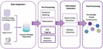
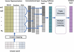
The goal of information extraction is to extract important information from text from a variety of data sources. The diversity of data from many sources makes this task complex, and there are several approaches for getting such information. This work’s information is in Thai, with complicated grammatical patterns and cultural term ambiguity. Pre-processing is necessary for Thai language work. There are no spaces between the words. A full stop is not used to signal the end of a sentence. When two words have the same meaning but are spelt differently or have many different names, the use of a part of speech can help to define the function of that word. Extracting useful data from numerous articles is still difficult after pre-processing. This research will use a new approach for more accurate information extraction. To make data more useful, the creation of a knowledge graph can be performed in other works with more complete data. Figure 1 shows an overview of the architecture of an information extraction system.

Figure 1 Architecture of the information extraction system.

The following are summaries of the primary modules of information extraction. The initial stage is to collect data from various sources and store it in the same data source. At this step, the structure of the data source that has to be stored, as well as the structure of the central data repository, must be known and built to support the data in preparation for data extraction. To be able to retrieve the necessary information using the designed structure. This process can retrieve data in many different ways, such as by accessing an API from a serviced data source or retrieving information from a website. When information is transferred to the same central repository. The following step is to perform a pre-process. This stage splits the article into sentences and tokens, then assigns the label to the POS and the position of the token based on the context of the word. The information extraction step is then started by extracting the name entity words from the repository. Then, discover name entity semantic relationships to create a triple relationship, which means there is a subject, a predicate, and an object. The extracted data in triples will be concatenated and stored in knowledge graph format as a source for future application development, and when new data becomes available, it will map the unseen word back to the vector to discover the next triple.

3.1 Data Integration

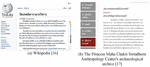
The initial stage is to integrate data from various sources. Data structures must be created to support the collected data. This paper will design data storage based on the Dublin Core metadata standard. The web crawling technique is used to obtain data from multiple sources by crawling the webpages of the various sources, as well as the API service, which is used to obtain data from data sources. Both approaches will collect data and map it to the same structure that was created. Figure 2 shows an example of data sources.

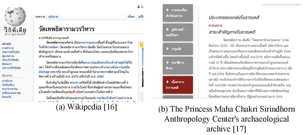
Figure 2 The examples of data sources.

3.2 Data Pre-processing

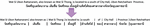
After the data integration phase, this step is to get data from the repository and tokenize or split a string or text into a list of tokens. We utilize tokenization dictionaries, which are excellent for languages that do not tokenize on whitespace and can handle spelling variants and technical vocabulary. Figure 3 shows an example of tokenization in Thai.

Figure 3 An example of tokenization in Thai.

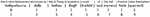
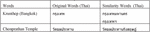
We define a label as part of speech (POS) after tokenization, which includes nouns, verbs, adjectives, adverbs, pronouns, prepositions, and conjunctions. This technique is useful for resolving lexical ambiguity because it assigns one part of speech to each word. Figure 4 shows an example of words with POS in Thai.

Figure 4 An example of words with POS.

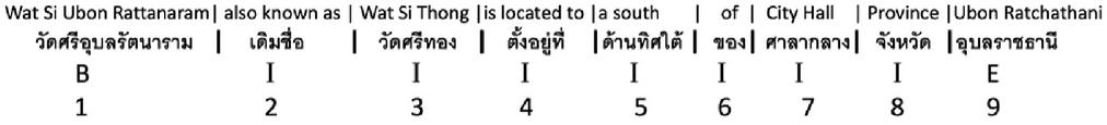
Figure 5 An example of words with position.

The position of the word in the sentence is labeled “B” for a subject word if it is at the beginning of the sentence, “I” for a predicate word if it is in the sentence, and “E” for an object word if it is at the end of the sentence, and another positioning is the position of the word in the sentence. Figure 5 shows an example of words with position.

3.3 Information Extraction

In this step, we utilize the results of the pre-processing data technique to discover semantic relationships between concepts using word vector representation, multiple instance learning (MIL), and unseen word mapping. Figure 6 shows the relation extraction system model.

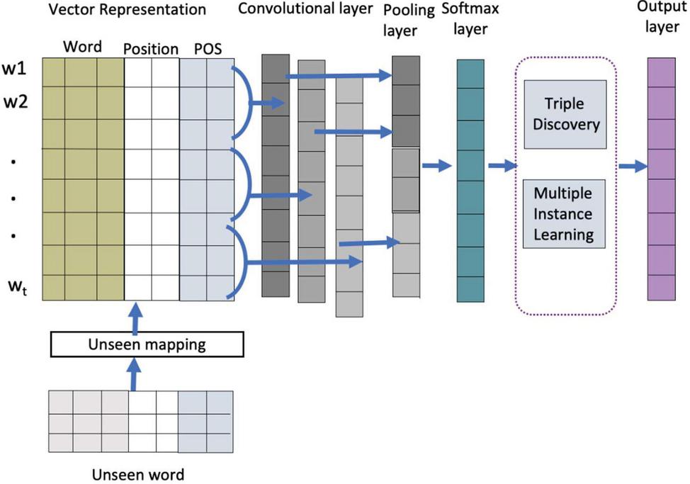
Figure 6 Model for relation extraction with a convolutional for CNN layer.

3.3.1 Input embedding layer

There are two main components: word embedding and word features. We use word2vec embedding, which is based on the Skip-gram model. Each word in a sentence is turned into a vector as e $_{i}$ , where V is the vocabulary size and m $_{e}$ is the word embedding dimension. Word features are POS features as d $_{1}$ and position features as d $_{2}$ where m $_{d}$ is the word feature embedding dimension.

This approach is used to turn words into matrices, which are subsequently utilized as inputs for the convolutional for CNN model. Let n be the length of the relations mentioned, and x $=$ [x $_{1}$ , x $_{2}$ ,…, x $_{n}$ ] be a relation mentioned with x $_{i}$ as the i-th word. The word embeddings e $_{i}$ and the word features d $_{1}$ and d $_{2}$ are concatenated into a single vector x $_{i}$ $=$ [e $_{i}$ , d $_{1}$ , d $_{2}$ ]. As a result, a matrix x of size (m $_{e}$ $+$ 2m $_{d}$ ) * n can be used to represent the sentence x. Then, feed this input matrix into the convolutional for CNN layer.

3.3.2 Convolutional for CNN layer

This process is important for merging all features and filtering them using a combination of weight vectors, bias, and a sliding window. The filter is represented as a weight matrix F $=$ [f $_{1}$ ,f $_{2}$ ,…,f $_{w}$ ] with w as the window size. Convolutional for CNN is done on each filter F to create a feature map s $=$ [s $_{1}$ , s $_{2}$ ,…,s $_{n - w}$ $_{+ 1}$ ]:

s_{i} = g (\sum_{j = 0}^{w - 1} f_{j + 1}^{T} + x_{j + i}^{T} + b)

(1)

Where b is a bias term and g is a non-linear function. We utilize n different weight matrix filters, and the process is repeated as many times as the total number of filters m.

3.3.3 Piecewise max pooling layer

In convolutional for CNN, a max pooling technique is frequently used to extract the highest values from each feature map. This layer tries to collect the most relevant features from each feature. The score sequence s of each filter f is passed through the max function to obtain a single value. This operation generates for each filter a single value as:

p_{f} = \max {s} = \max {s_{1}, s_{2}, \dots, s_{n - w + 1}}

(2)

3.3.4 Softmax layer

To express the relation mentioned, we concatenate the pooling scores for each filter into a single vector z $=$ [p $_{1}$ , p $_{2}$ ,…, p $_{m}$ ]. The number of filters in the model is denoted by n, and the pooling score of the i-th filter is denoted by p $_{i}$ . We use dropout on z during training. The softmax classifier’s output can be formalized as:

p = softmax (W_{1} (z * r) + b 1)

(3)

where p is the output, b denotes a bias, and W $_{1}$ denotes the transformation weight matrix. We perform an operation on z, where r is a vector of Bernoulli random variables, each of which has a probability p of being 0.

3.3.5 Semantic triple discovery

The semantic triple concept is discovered from the vector in this step. We start by capturing the similarity of entities using the similarity measure approach. The trained word embedding similarity measure is a real-valued function that measures the similarity between two entities. Cosine similarity is commonly used to assess semantic similarities. The cosine similarity of two vectors of characteristics A and B, where A and B represent entities, is expressed using a dot product as:

similarity = \cos (θ) = \frac{A \cdot B}{| A | | B |}

(4)

After the discovery of similarity entities, we capture the relationship between entities by comparing their assessments of relational similarity using word analogy. The degree of similarity of one word pair (A, B) to another is used to predict relationship similarity. The parallelogram model connects the two pairs of words (A: B and C: D), where A, B, C, and D represent entities. The difference vectors ( $\vec{B}$ – $\vec{A}$ and $\vec{D}$ – $\vec{C}$ ) are similar in the same relation as another pair. For example, Doi Suthep is in Chiang Mai, and Laem Promthep is in Phuket, so the place-city-city relationship is:

vec(“Doi Suthep”) $-$ vec(“Chiang mai”)
$\approx vec(“Laem Promthep”) - vec(“Phuket”)$	(5)

where vec( ) denotes as vector operator.

We use the pair difference operator (PairDiff) to detect syntactic and semantic analogies. This operator measures the cosine similarity between the two vectors corresponding to the difference between the word representations of the two words in each word pair. PairDiff is used to detect semantic analogies and is given by:

PairDiff (A : B, C : D) = \cos (B - A, D - C)

(6)

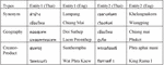
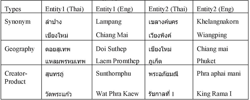
We can capture the semantic and syntactic relationships between entities using the PairDiff technique. The types of analogies and instances of analogies are shown in Table 1.

Table 1 Analogy types and instances examples

images

We focus on the elements in a semantic triple consisting of the subject (S), predicate (P), and object (O). We are given a new semantic triple of the form: A:P:B :: C:P:D, where P is a predicate of the triple. For example, in the case of (Wat Phra That Hariphunchai: Founder: King Athitayarai) and (Wat Niwet Thammaprawat: Founder: King Chulalongkorn), we compute the embedding offsets between the entities and predicates of each pair as follows:

\vec{A} - \vec{P} \approx \vec{B} - \vec{P} and \vec{P} - \vec{C} \approx \vec{P} - \vec{D}

(7)

3.3.6 Multiple instance learning

Following the semantic relation discovery step, problems with terms that do not reflect the meaning relationship frequently occur. To address these issues, we utilize multiple instance learning (MIL) by focusing on the relationship between entities on POS (Part of Speech) using only three tags (NN:noun, VB:verb, and ADV:adverb) but none of the other tags (Negative Otherwise). The categorization is as follows:

P_{b a g, i} {\begin{matrix} P O S, & i f P_{b a g, i} = {(N N_{1}, V B_{1}, A D V_{1}), \\ (N N_{2}, V B_{2}, A D V_{2}), \dots \\ (N N_{n}, V B_{n}, A D V_{n})} \\ N E G, & O t h e r w i s e \end{matrix}

(8)

We define the score function of the entity pair and its corresponding relation P (predicate) using the maximum operator:

P = \max (p_{i})

(9)

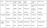
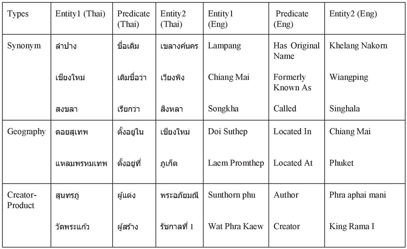
Table 2 shows the example of semantic relation triple from relation extraction.

Table 2 Examples of semantic relation triple extraction

images

3.3.7 Mapping unseen words to trained embedding

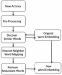
Finding a relationship will be more challenging when there is new information. If the word does not exist in the initial set of training, it will require a lot of resources and time to retrain. To solve this problem, we utilize the unseen mapping technique. Figure 7 shows an overview of mapping an unknown word system, and a detailed description of the model follows:

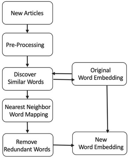
Figure 7 Overview of mapping an unseen word system.

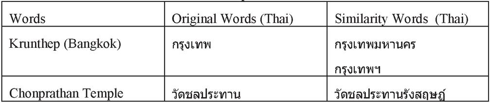
When new data reaches, the first step is to feed it into the pre-processing step, which is to tokenize the word, label the POS and position, and then enter the unseen mapping process, as shown below. Compare new word sets with existing word sets to check for duplicate words and to create just a new set of words where O is a word at the word embedding and T is a new word so that T-O equals a word unique to the word embedding. Then, to discover similar words, utilize words that do not appear in the existing word embedding. We extract n-grams from words and calculate their similarity values using character-level information representation.

The similarity function is shown as follows, where s $_{1}$ and s $_{2}$ are the words to be compared. Table 3 contains examples of similar words.

Similarity (s_{1}, s_{2}) = \frac{2 * | p a i r s (s 1) \cap p a i r s (s 2) |}{| p a i r s (s 1) | + | p a i r s (s 2) |}

(10)

Table 3 The example of similar words

images

Where words are similar, we add the unseen words to O as the same value of word similarity. Next, we use the nearest neighbor word mapping method by using words in O with their features. The pseudo code for this method is given below:

Algorithm 1 Unseen mapping prediction

New Article Semantic Relation Triple Step 1: The words in O (O is a word at word embedding) can be both ‘Subject’ and ‘Object’. We use position to define them.

‘Subject’ = {noun, B: B represents the beginning of a sentence.}

‘Predicate’ = {noun, verb, adverb, I: I represents the inside of a sentence.}

‘Object’ = {noun, E: E represents the ending of a sentence.}

Step 2 : If it is ‘Subject’, we slide to right way for finding the ‘Predicate’ and ‘Object’.

Step 3: If it is ‘Object’, we slide to the left way for finding the ‘Predicate’ and ‘Subject’.

Step 4: If it is ‘Predicate’, we can slide to left way for finding ‘Subject’ and right way for finding ‘Object’.

Then, we add the unseen words to O as the same value of nearest neighbor word. Finally, we can obtain the new relationship between entities without training all of the word embedding, which saves a significant amount of time and resources.

3.4 Post-Processing

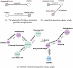
The final process is to construct a knowledge graph based on the extracted relationships, which are represented in triple form as subject, predicate, and object. It is possible for the same word to be both the subject and the object in each triple. Figure 8 shows an example of a cultural heritage knowledge graph created with the triple mapping approach.

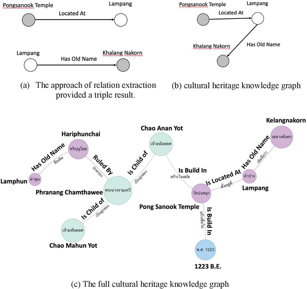
Figure 8 An example of a cultural heritage knowledge graph.

For each triple, we construct two new nodes, one for the subject entity as N1 and one for the object as N2, which are connected by the given relation r. Each triple will be compared to the knowledge graph G and combined. This method’s pseudo code is as follows:

Algorithm 2 Knowledge graph construction

Semantic Relation Triple Cultural Heritage Knowledge Graph Step 1: We define the starting point of the knowledge graph by creating the first node as a culture node and relation with four domains as place node, artifact node, event node and people node. Step 2: Define a triple of each domain as the result of relation extraction, where the “Subject” is node N1, the “Object” is node N2, and the “Predicate” is the relationship between them, replaced by R. Step 3: Choose the first triple of each domain to operate as the knowledge graph’s initial stage, denoted by G. Step 4: Each node will be assigned to G. If N1 and N2 match to nodes in G., then combine them and add the relation R. Step 5: If Ni does not match any nodes in G. We merge them with domain node.

4 Experimental Results

We present our experiments in this section. We provide an overview of the training dataset, parameter settings, and experiment results.

4.1 Parameter Settings

The parameters are tuned in a grid search to find the best combination of parameters. Table 4 lists some of the results including the top 10 F1 scores.

Table 4 Parameter-tuning results

Parameters
	Word	Word	Position	Dropout
Architecture	Size	Dimension	Dimension	Operation	P	R	F
CBOW	2	100	4	0.1	0.67	0.69	0.67
	3	100	5	0.5	0.71	0.65	0.69
	2	200	4	0.1	0.51	0.78	0.62
	3	200	5	0.5	0.65	0.66	0.65
Skip-gram	2	100	4	0.1	0.66	0.64	0.65
	3	100	5	0.5	0.73	0.78	0.75
	2	200	4	0.1	0.71	0.71	0.71
	3	200	5	0.5	0.76	0.72	0.74
	2	300	4	0.1	0.66	0.73	0.70
	3	300	5	0.5	0.68	0.67	0.68

After training models with different combinations of parameters. We utilize the Skip-gram model, which has 100 dimensions, position dimensions is 5, window size is 3, and a dropout rate of 0.5. Table 5 shows all of the parameters and their respective ranges and displays the parameter the best aspect model.

Table 5 The parameter ranges used for aspect model and the parameters of best aspect model

Parameter	Range	Best Value
Architecture	Skip-gram [7], CBOW [7]	Skip-gram
Word Size	2 to 5	3
Word Dimension	100, 200, 300	100
Positon Dimension	2 to 5	5
Dropout Operation	0.1 to 0.5	0.5

4.2 Dataset

We evaluate our model on three cultural heritage datasets from Thailand’s Ministry of Culture’s Cultural Knowledge Archive. This archive is divided into four categories: artifacts, people, places, and events. The Princess Maha Chakri Sirindhorn Anthropology Center’s archaeological archive focuses on places. The last data is taken from Wikipedia, and we use place, event, and person subjects from the cultural heritage domain. We divided the data into testing and training datasets, with 70% used for training as a relation extraction technique and 30% used for evaluation as unseen words. The total number of datasets is shown in Table 6.

Table 6 Thai cultural datasets

Data	Subject of Articles	Number of Articles
Cultural knowledge center	Places, Events, Person, Artifact	5,000
Archaeology database	Places, Artifacts	1,500
Wikipedia	Places, Events, Person	3,000

4.3 Main Results

The data for the experiment in this work was divided according to the topic type of the data: location, person, activity, and artifact. The precision (P), recall (R), and F1 (F) score measures were used to evaluate the experimental data. As shown in Table 7, two experiments were carried out with relation extraction and an experiment with unseen word mapping and ROC Curves as shown in Figure 9.

Table 7 The accuracy of our relation extraction system for each data type and unseen word prediction

		Semantic Triple			Unseen Word
		Relation Extraction			Prediction
Domain	Number of Relation	P	R	F	P	R	F
Place	1431	0.91	0.89	0.90	0.82	0.86	0.84
Artifact	240	0.87	0.89	0.88	0.81	0.87	0.84
People	776	0.89	0.90	0.89	0.77	0.87	0.82
Event	469	0.89	0.86	0.88	0.85	0.88	0.87

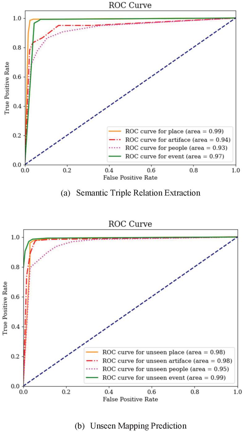
Figure 9 Roc Curves of relation extraction method and unseen mapping prediction method.

The “place” relationship was extracted with the largest and best accuracy from Table 3, with an F1 value of 0.90. We found that the greatest information can be extracted about “location,” “ownership,” and “creation time”. “Person” with an F1 value of 0.89 can extract relationships related to family relationships, such as being a child of, father of, or mother of. “Artifact” and “Event” have the same F1 value of 0.88. The “Artifact” can extract relationships related to ownership or the creator, whereas the “Event” will be related to the time of the events. “Event” prediction was the most accurate for unseen word prediction, with an F1 score of 0.87. The F1 score for “Artifact” and “Event” were both 0.84. “People” had the lowest F1 score of 0.82. Because events have unique names, “Event” has a greater accuracy than other data types. As a result, they are easier to map than other various data types, especially as Thai names are quite complicated.

To evaluate the proposed method’s overall performance, we compare it to baseline approaches for both relation extraction and unseen word prediction. The data was randomly divided into three datasets across four domains for our evaluation: place, artifact, people, and event. Tables 8 and 9 show the results of the comparison.

Table 8 The accuracy of our relation extraction method compare with baseline methods

	CBow	Skip-gram	Skip-gram with Word Feature and MIL (Proposed Method)
Datasets	P	R	F	P	R	F	P	R	F
Dataset1	0.73	0.68	0.71	0.76	0.78	0.77	0.89	0.88	0.89
Dataset2	0.72	0.65	0.69	0.71	0.78	0.75	0.89	0.88	0.88
Dataset3	0.71	0.62	0.66	0.71	0.77	0.74	0.89	0.88	0.89
Average	0.71	0.65	0.69	0.73	0.78	0.75	0.89	0.88	0.89

Table 9 The accuracy of our unseen mapping method compare with the other baseline method

				Unseen Mapping
	Fastext			(Proposed Method)
Datasets	P	R	F	P	R	F
Dataset1	0.80	0.88	0.82	0.81	0.87	0.84
Dataset2	0.79	0.75	0.77	0.81	0.86	0.83
Dataset3	0.78	0.74	0.76	0.81	0.87	0.84
Average	0.79	0.79	0.79	0.81	0.87	0.84

Our approach extracts data from three test datasets with success. The accuracy of each test data set was not significantly different, with an average precision of 0.89, recall of 0.88, and F1 of 0.89, whereas the other methods for each dataset were different, but the average accuracy was still less than our method. As a result, our method has defined word features to improve the accuracy of relationship extraction. Furthermore, utilizing multiple instance learning, meaningless relationships can be eliminated, and the quality of the relationship can be expressed more accurately.

In each of the datasets tested, our unseen mapping approach can detect the relationship of data that has never been trained before. It was found that the efficiency was not much different each time. The average precision is 0.81, recall is 0.87, and F1 is 0.84, while Fastext has variable performance across datasets, making the average efficiency less. Our method begins by removing duplicate words, which reduces the amount of data that must be examined. Our technique includes a word feature that can indicate the function of the word, allowing us to extract words and find the relationship more accurately.

5 Conclusions

This paper introduces a new model for extracting relationships between entities as semantic triples from cultural heritage archives. Word tokens and word features as part of speech tagging and word position tagging are used as inputs for our model. We use POS to understand the type of word. Using the position of a word indicates the word functions in the meaning of the sentence. Subject words often occur at the beginning of a sentence, while predicate words often occur in the middle of the sentence and object words often occur at the end of the sentence; also, the position of words in a sentence is the principal means of showing their relationship. We apply multiple instances learning (MIL) to deal with problems of words that do not express relationships. We cluster the specific words to discover the predicate word by eliminating the words that are not relevant between subject and object. Besides, the problem of using word vector is the performance of relation extraction drops when the words do not appear or unseen words in the training dataset. We relieve this problem by mapping the unseen words to trained embeddings. The unseen word mapping filters the trained words and concatenates new words to word embeddings. The correlation extraction accuracy of our model was 0.89, recall was 0.88, and F1 was 0.89, according to the test results. Pre-processing as a part of speech improves the accuracy of identifying the function of the word to discover the name entity, and word position will assist us in determining the function of the Subject, Predicate, and Object words in a relationship. Furthermore, after the relationship set is generated, the addition of multiple instance learning aids in the elimination of meaningless relationships. When compared to other correlation extraction methods, it also helps to strengthen the relationship more correctly. The accuracy of the unseen word prediction is 0.81, the recall is 0.87, and the F1 is 0.84. It is more accurate than other methods because duplicate words are deleted when new information is received and mapping similar words with the word feature attached makes the relationship more accurate. This method can reduce processing time and resources for data training versus resource.

We will develop our approach in the future to be able to use cultural information with other languages that have different grammatical structures and can be more complicated, as well as to focus on extracting more different relationships. To be able to link data that shows a broad relationship and to be more accurate in extracting correlations.

Acknowledgement

The authors would like to extend our sincere appreciation to Assoc. Prof. Dr. Suchada Sitjongsataporn for her patience, guidance, and support. We have benefited greatly from your wealth of knowledge and meticulous editing.

References

[1] What is meant by “cultural heritage” from www.unesco.org [online]. Access on December 27, 2021.

[2] Marcos Garcia: Semantic Relation Extraction.Resources, Tools and Strategies, Computational Processing of the Portuguese Language, Volume 9727, 2016.

[3] Tiezheng Nie, Derong Shen, Yue Kou, Ge Yu and Dejun Yue: An Entity Relation Extraction Model Based on Semantic Pattern Matching, Eighth Web Information Systems and Applications Conference, 2011.

[4] Huu Nguyen, T., Grishman, R.: Relation Extraction. Perspective from Convolutional Neural Networks. the 1st Workshop on Vector Space Modeling for Natural Language Processing, 2015.

[5] Khashabi, D. On the Recursive Neural Networks for Relattion Extraction and Entity Recognition, 2013.

[6] Pennington, J., Socher, R., Manning, C.: GloVe. Global Vectors for Word Representation. Conference on Empirical Methods in Natural Language Processing (EMNLP), 2014.

[7] Mikolov, T., Chen, K., Corrado, G., Dean, J. Efficient estimation of word representations in vector space. ICLR Workshop, 2013.

[8] Xia, Y., Liu, Y. Chinese Event Extraction Using DeepNeural Network with Word Embedding. ArXiv, 2016.

[9] Soni, A., Viswanathan, D., Shavlik, J., Natarajan, S. Learning Relational Dependency Networks for Relation Extraction. Inductive Logic Programming, 2017.

[10] Nguyen, D., Verspoor, K. Convolutional neural networks for chemical-disease relation extraction are improved with character-based word embeddings. In Proceedings of the 17th ACL Workshop on Biomedical Natural Language Processing (BioNLP), 2018, pages 129–136.

[11] Bouraoui, B., Jameel, S., Schockaert, S. Relation Induction in Word Embeddings Revisited. Proceedings of the 27th International Conference on Computational Linguistics, 2018.

[12] Zied Bouraoui, Shoaib Jameel, Steven Schockaert: Probabilistic Relation Induction in Vector Space Embeddings, https://arxiv.org/, 2017.

[13] Gormley, M., Yu M., Dredze, M. Improved Relation Extraction with Feature-Rich Compositional Embedding Models. Proceedings of the 2015 Conference on Empirical Methods in Natural Language Processing, 2015.

[14] Buranasing, W., Phoomvuthisarn, S. Information Extraction for Cultural Heritage Knowledge Acquisition using Word Vector Representation. International Conference on Complex, Intelligent and Software Intensive Systems, 2018.

[15] Choi, D., Choi, K. Automatic Relation Triple Extraction Dependency Parse Tree Traversing. the 16th International Conference on Knowledge Engineering and Knowledge Management Knowledge Patterns, 2008.

[16] Wikipedia from https://th.wikipedia.org/wiki [online]. Access on December 30, 2021.

[17] The Princess Maha Chakri Sirindhorn Anthropology Center’s archaeological archive from https://www.sac.or.th [online]. Access on December 30, 2021.

Biographies

Watchira Buranasing is a Ph.D. student at Mahanakorn University of Technology in Bangkok, Thailand. She works at the National Electronics and Computer Technology Center as a research assistant. Her current areas of interest in study include digital archives and semantic technology.

Woraphon Lilakiatsakun received a Ph.D. in Telecommunication Engineering from the University of New South Wales in Australia. He is an assistant professor at Mahanakorn University of Technology’s Faculty of Engineering and Technology in Bangkok, Thailand.