Video Face Detection Based on Improved SSD Model and Target Tracking Algorithm
Yilin Liu, Ruian Liu*, Shengxiong Wang, Da Yan, Bo Peng and Tong Zhang
College of Electronic and Communication Engineering, Tianjin Normal University, Tianjin, 300387, China
E-mail: 574677370@qq.com; ruianliu@sina.com; shengxiong1818@163.com; 1003143193@qq.com; pengboiu@163.com; 1450018535@qq.com
*Corresponding Author
Received 28 October 2021; Accepted 15 November 2021; Publication 19 January 2022
Abstract
Video face detection technology has a wide range of applications, such as video surveillance, image retrieval, and human-computer interaction. However, face detection always has some uncontrollable interference factors in the video sequence, such as changes in lighting, complex backgrounds, and face changes in scale and occlusion conditions, etc. Therefore, this paper introduces deep learning theory and combines the continuity characteristics of video sequences to make related research on video face detection algorithms based on deep learning. First, this algorithm uses the residual network as the basic network of the Single Shot MultiBox Detector (SSD) target detection network model and trains a Rest-SSD face detection model to detect faces. Experimental results show that the method can achieve real-time detection and improve the accuracy of video face detection, which is required for face detection in a video. Then we based on the continuity characteristics of video sequences. This paper proposes a video face detection method based on the training of the Rest-SSD face detection model. The method first uses kernel correlation filtering to track consecutive n frames according to the detection results, sets weights on the confidence of the n frames of tracking results, uses the weighted average method to calculate the best tracking result, and then sets the best tracking result confidence and the current frame sets the appropriate weights for the confidence of the detection result for fusion, thereby improving the video face detection accuracy.
Keywords: Deep neural network, SSD target detection, continuous frame target tracking, kernel correlation filtering.
1 Introduction
Face detection means to determine whether a human face is located within an image by carefully observing the image after analysis and processing. If faces are detected, the size and location information of all the faces should be recorded [1, 2] and marked within the image. However, for face detection in a video, the determination is no longer based on a still face image but a dynamic video file; therefore, face detection in a video requires real-time detection. Moreover, for many problems such as scale changes of faces within the video, variable and complex backgrounds and obscured faces, the images of a single frame cannot provide comprehensive information; therefore, researchers have paid more attention to video face detection using continuity features of video sequences.
Since the 1990s, scholars in the field of face information research have focused their research on face detection [3], and the main idea of deep learning is to build artificial neural networks and train them based on the calibrated target locations, which are eventually used for target detection. In 2013, RossGirshick et al. proposed a target detection algorithm, namely R-CNN (Region-CNN) [4], which uses convolutional neural networks for the target detection task and paves the way for some subsequent algorithms, such as Fast-RCNN [5], SPP-NET [6], and Faster-RCNN [7], etc. The Face R-CNN [8] method is based on the Faster R-CNN framework for face detection and is optimized for face detection Cascade CNN is a representative of the transition from traditional detection to deep networks [9], which uses a cascade to organize multiple classifiers, where each level of the classifier consists of a convolutional neural network and constructs an image pyramid, and sends the region to be detected into three networks for regression correction through a sliding window, and usually the first network can eliminate most negative samples, while The NMS (Non-Maximum Suppression) algorithm is used between each network to remove the regions with more overlap. The subsequent MTCNN network [10] also borrows the idea of the Cascade CNN model. In the subsequent study [11], a total loss function combining L2 loss and triadic loss was used to reduce the missed detection; in the literature [12], a two-layer cascade network was also used; in the literature [13], an image pyramid was added between the cascade networks; all these improvements achieved better detection results. In terms of accuracy, the deep learning-based face detection model is much higher than the traditional face detection model. However, in terms of detection speed, the former is slower than the latter. Even if GPU is used, it is not possible to achieve real-time in practical use.
The deep learning-based face detection method is more capable of meeting the needs of complex environments within videos, but its shortcoming is that it is computationally intensive and cannot achieve real-time face detection. At this stage, there is a lot of work to optimize the detection speed. Among these methods, the best performers include YOLO (You Only Look Once) [14] and SSD (Single ShotMulti-boxes Detector) [15] neural network target detection models. The disadvantage is that it is computationally intensive and cannot achieve real-time face detection. At this stage, there is a lot of work to optimize the detection speed, and YOLO has a more common detection accuracy compared with Faster-RCNN [16], but the detection is faster. The main content of this research paper.
In this paper, we improve the SSD target detection model and successfully introduce it to the face detection task, proposing an improved SSD face detection method. The method replaces the VGG [17] base network in the classical SSD target detection framework with a ResNet residual network structure to extract the corresponding features, and then the extracted features are fed into the prediction network for detection [18]. Second, a video face detection method that fuses the target tracking results is proposed based on the trained Rest-SSD detection model using the temporary and spatial features of video sequences. This method firstly takes the detection results as the basis, uses correlation kernel filtering for tracking n consecutive frames, sets weights for the tracking confidence of n frames, uses weighted averages to calculate the best tracking results, considers the tracking results as the prediction of face information in previous frames to face information in the current frame, and then fuses the best tracking results and the current frame detection results by setting certain weights, so as to improve the video face detection accuracy.
2 Related Work
This paper adopts a deep learning based face detection method, and within this section, it will focus on the classical SSD network structure, non-maximal value suppression and evaluation metrics for face detection.
2.1 Classical SSD Network Structure
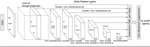
Figure 1 [19] shows the SSD network model, which is mainly divided into two parts: the base and prediction networks. The base network is a deep CNN located at the front end, which uses the image classification network VGG16 with the classification layer removed for initial feature extraction; the prediction network is a cascaded CNN located in the back end, which can extract features at different scales from the feature layers generated by the base network and perform multiple detection.
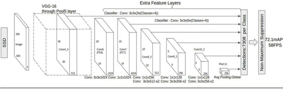
Figure 1 Classical SSD network structure.
2.2 Non-extreme Value Suppression
Searching for local maxima and suppressing non-maximal elements is known as non-maximal suppression. The goal of face detection is to find the ideal position for identifying faces by searching for and keeping the optimal frame among multiple detection frames and removing the redundant ones. The process of non-maximum suppression is described as follows.
1. The predicted frames are sorted from the highest to lowest values according to the principle of confidence;
2. The predicted frame with the highest confidence value is selected as the output frame for face detection;
3. The area of all the predicted frames is determined.
4. The intersection area of the output frame for face detection and the other predicted frames is divided by their concatenated areas to obtain the Intersection-over-Union (IoU) value.
5. Predicted borders whose IoU exceeds the set threshold value are deleted.
6. The abovementioned process is repeated until all the borders are output.
Figure 2 shows the results of face detection using non-maximal suppression. Five prediction frames are output for the faces in the figure. All the prediction boxes are sorted from the largest to smallest. The results are set as A 0.98, B 0.83, C 0.81, D 0.75 and E 0.67, and the highest score A 0.98 is selected as the output frame for face detection; the area of all the frames is calculated, and if the overlap area (IOU) with frame A is larger than the set threshold (generally 0.65), we delete the box. For example, calculate the IOU of box A and the rest of the B, C, D and E boxes, A and B, D IOU threshold, delete B, D boxes, the remaining A, C, E boxes; from the IOU less than the threshold of C, E boxes continue to select a confidence score of the highest box, repeat the process has been above, keep the C box to delete the E box; finally leaving A, C two boxes.

Figure 2 Non-maximum suppression of face detection results.
2.3 Evaluation Indexes of Face Detection
The metrics of face detection model evaluation include face accuracy, face detection rate and detection time. Among them, the face detection rate is the percentage of detected faces out of the total number of faces, also called Recall; the face accuracy rate is the proportion of the actual number of faces out of the total number of detected faces. Generally speaking, the performance of models with high accuracy and detection rates is more outstanding. The ROC curve can also be used to evaluate the model, which is a coordinate system consisting of the detection rate as the vertical coordinate and the percentage of false detections among the total number of non-faces as the horizontal coordinate, which is the “subject operating characteristic” (ROC). It is the abbreviation of the “Receiver Operating Characteristic” curve.
3 Proposed Methods
3.1 Dataset Preprocessing
The images of the WiderFace dataset [20] are selected from public places, and there are 61 images of scenes, such as traffic and party images; there are also faces with different postures, scales and numbers within the same image, among which the percentages of the validation, training and test sets are 10%, 40% and 50%, respectively. Because the real label information of the face frame is not provided within the test set, this experiment treats the validation set as the test set and verifies the experimental results. The FDDB dataset [21] is mainly used for constrained face detection research, which selects 2845 images taken in the field environment, from which 5171 face images are selected. It is a widely used and authoritative face detection platform.
3.2 Loss Function
Let denote the i-th preset frame matching the j-th real face label frame, a label frame can match more than one preset frame, so there is . The total loss function is the weighted sum of the localization loss (loc) and confidence loss (conf), and the expression is shown in Equation (1).
| (1) |
In this equation, is the total number of predefined frames that can be matched with the real face label frame is represented, and if the value is 0, the loss value is 0 and the weight factor is set to 1. The localization loss represents the loss between the real face labeled border parameter and the predicted border . The prediction frame is actually a regression of the width , center and height of the predefined border, which can be seen in Equation (2).
| (2) |
In this case, represents the offset between the predicted frame and the mth predefined frame. The reason for optimizing the localization loss function is to obtain the optimal to minimize the localization loss . represents the offset between the real labeled frame of the face and the mth predefined frame. Relying on Equations (3), (4), the parameter of the offset value can be calculated.
| (3) | |
| (4) |
In this, represents the width, height and center point coordinates of the real face label box, respectively, and represents the width height and center point coordinates of the preset box, respectively. Based on the following Equation (5), the loss can be obtained:
| (5) |
Since there are only faces and backgrounds in the face detection task, the confidence loss is the binary confidence softmax loss, as shown in Equation (6):
| (6) |
Where the value of takes 1 means that the i-th preset box matches to the j-th face real label box, means the confidence of the i-th preset box corresponding to the face, means the function of positive or negative samples, and the first half of the formula is the loss of positive samples, i.e., the loss of the face, and the second half is the loss of negative samples, i.e., the loss of the background.
3.3 Matching Strategy
During training, real label frames need to be created to correspond with the present frames. The matching strategy of the Rest-SSD face detection network is as follows.
First, the position of the present box with the most obvious IoU (overlap rate) with the real labeled box on the face is specified, and it is taken as the initial match for this labeled box. In this way, multiple face frames within the image will form multiple such matches to ensure that all face frames have a present box that can achieve a match. In general, the present box that can match the real face label box is called a positive sample, otherwise it is a negative sample. In the second step, the remaining present frames that do not achieve a match are searched for and the face real label frame whose IoU exceeds a certain threshold value is used as the matching frame. In this way, the label frame can be matched with several predefined frames. It is necessary to ensure that a face real label box can achieve matching with several preset boxes. However, if a preset box can achieve matching with several label boxes, the preset box can only achieve matching with the face real label box with the largest IoU, and the threshold value is set to 0.5 here.
3.4 Set the Scale and Aspect Ratio of the Preset Box
The required face present frame in this paper does not correspond to the actual perceptual field of each layer of the network. Assuming that m feature maps are predicted, the scale of the present frame within each layer of the feature map can be found according to the following Equation (7):
| (7) |
The values of and are taken as 0.2 and 0.9, respectively, which represent the lowest and highest prediction convolutional layers with scales of 0.2 and 0.9, respectively, and the scales of all the prediction layers in the middle have a linear increasing trend. The width-to-height ratio used should also change when the prediction frame is different. Assuming that the width-to-height ratio is , then the height of either prediction frame can be found by the formula: , and the formula for its height is . In this case, represents the actual size of the present box calculated by multiplying the image size and the scale . If the aspect ratio is 1, then a square preset box with scale is added. In this way, six present boxes are formed at each feature map position. Assume that the center of all the present boxes is in which represents the kth square feature map. In fact, to get the optimal values of the scale and aspect ratio of the present boxes, they should be carefully designed with a specific data set.
3.5 Network Structure
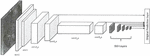
This paper replaces the base network in the original SSD network model with residual network (ResNet18) for initial extraction of face features to prevent network degradation as the layers of the deep CNN deepen; Figure 3 shows the network model. The base network is ResNet18, a residual network with a shortcut connection structure, and the prediction network is still a five-layer SSD-enhanced convolutional layer to extract different scale features and perform multiple detection tasks.
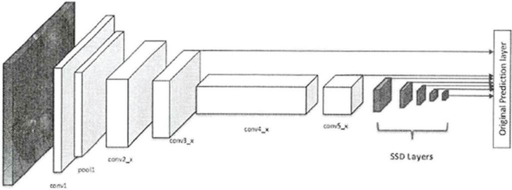
Figure 3 Improved SSD network structure.
The image input to the RestNet18 residual network passes through 7 7 64 convolutional layers, then through building blocks, each of which has 2 layers, so there are layers, and finally, there are average pooling (fc) layers for 18 layers of neural network feature units, of which the first 17 layers are used for feature extraction and the last layer is used for output. The improved SSD face detection uses the first 17 layers of ResNet18 as the base network, and its specific base network structure is shown in Table 1.
Table 1 Basic network structure table
| Layer Name | Layer Type | Core Size/Step/Fill | Output Feature Map Size |
| Input Image | RGB Pictures | – | 3 300 300 |
| Convl/relu1 | Convolution/ReLu | 64 7 7/2/3 | 64 300 300 |
| Pool | Max pooling | 64 3 3/2/1 | 64 150 150 |
| Conv2_l/relu2_1 | Convolution/ReLu | 64 3 3/1/1 | 64 150 150 |
| Conv2_2/relu2_2 | Convolution/ReLu | 64 3 3/1/1 | 64 150 150 |
| Conv3_1/relu3_1 | Convolution/ReLu | 128 3 3/2/1 | 128 75 75 |
| Conv3_2/relu3_2 | Convolution/ReLu | 128 3 3/1/1 | 128 75 75 |
| Conv4_1/relu4_1 | Convolution/ReLu | 256 3 3/2/1 | 256 38 38 |
| Conv4_2/relu4_2 | Convolution/ReLu | 256 3 3/1/1 | 256 38 38 |
| Conv5_1/relu5_1 | Convolution/ReLu | 512 3 3/2/1 | 512 19 19 |
| Conv5_2/relu5_2 | Convolution/ReLu | 512 3 3/1/1 | 512 19 19 |
Behind the basic network, the prediction network structure adds a series of multiscale convolutional feature layers, which differ in convolutional kernel size, step size and padding. Table 2 shows the multiscale feature layers of the prediction network, where conv6_2, conv7_2, conv8_2, conv9_2 and conv10_2 are connected to the convolutional detector as the feature layers to be predicted for detecting the picture of the face. Additionally, conv3_x and conv5_x of the base network are also used as the convolutional feature layers of the scale.
Table 2 Forecast network structure table
| Layer Name | Layer Type | Core Size/Step/Fill | Output Feature Map Size |
| Conv6_l/relu6_1 | Convolution/ReLu | 1024 3 3/1/6 | 1024 19 19 |
| Conv6_2/relu6_2 | Convolution/ReLu | 1024 1 1/1/0 | 1024 19 19 |
| Conv7_l/relu7_1 | Convolution/ReLu | 256 1 1/1/0 | 256 19 19 |
| Conv7_2/relu7_2 | Convolution/ReLu | 512 3 3/2/1 | 512 10 10 |
| Conv8_l/relu8_1 | Convolution/ReLu | 128 1 1/1/0 | 128 10 10 |
| Conv8_2/relu8_2 | Convolution/ReLu | 256 3 3/1/0 | 256 5 5 |
| Conv9_l/relu9_1 | Convolution/ReLu | 128 1 1/1/0 | 128 5 5 |
| Conv9_2/relu9_2 | Convolution/ReLu | 256 3 3/1/0 | 256 3 3 |
| Conv10_l/relu10_1 | Convolution/ReLu | 128 1 1/1/0 | 128 3 3 |
| Conv10_2/relu10_2 | Convolution/ReLu | 256 3 3/1/0 | 256 1 1 |
As the scale, number and aspect ratio of the preset boxes in the feature maps of different scales differ, the parameters of the preset boxes in each layer also differ, and their set parameters are presented in Table 3.
Table 3 Preset frame parameter settings
| Feature | Preset | Aspect Ratio | Number of | |
| Layer Name | Map Size | Box Size | of Preset Boxes | Preset Boxes |
| Conv3_2/relu3_2 | 75 75 | 3060 | {1,2,1/2} | 75 75 4 22500 |
| Conv5_2/relu5_2 | 19 19 | 60111 | {1,2,3,1/2,1/3} | 19 19 6 2166 |
| Conv6_2/relu6_2 | 19 19 | 111162 | {1,2,3,1/2,1/3} | 19 19 6 2166 |
| Conv7_2/relu7_2 | 10 10 | 162213 | {1,2,3,1/2,1/3} | 10 10 6 600 |
| Conv8_2/relu8_2 | 5 5 | 213264 | {1,2,3,1/2,1/3} | 5 5 6 150 |
| Conv9_2/relu9_2 | 3 5 | 264315 | {1,2,1/2} | 3 3 4 36 |
| Conv10_2/relu10_2 | 1 1 | 315366 | {1,2,1/2} | 1 1 4 4 |
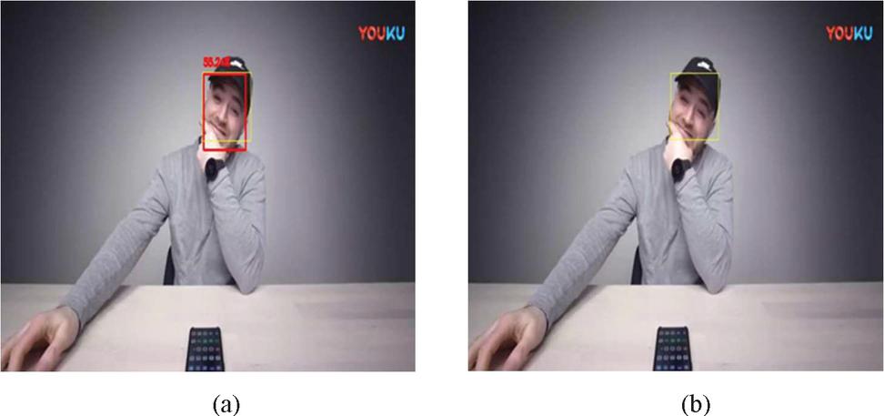
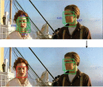
Figure 4 (a) Results of simultaneous face tracking and detection in the Tth frame; (b) Results of simultaneous face tracking and detection in the T 1th frame.
3.6 Video Face Detection Algorithm Incorporating Continuous Frame Target Tracking Results
Video face detection in the video face detection due to the special characteristics of the video sequence, the face is constantly moving, there will be missed detection due to incomplete display of the positive face or semi-obscured. Therefore, we consider the target tracking algorithm as a temporal feature to be added to the video face measurement to improve the video face detection accuracy and avoid missed detection. As shown in Figure 4(a), when face detection and tracking are performed simultaneously, both detection and tracking can be well achieved in the Tth frame of the video, but as shown in Figure 4(b), the face is not detected but the tracking result appears in the T 1th frame, so the face tracking result can predict the face position in the next frame to strengthen the detection confidence and thus improve the face detection accuracy in the video.
The tracking algorithm is used in this study to improve the accuracy of the detection algorithm. First, each detection result in each frame is the target to be tracked, and it is used as the starting point to implement the target tracking for a continuous m frames. In this way, except for the m-frames at the beginning and end of the video, each frame has the tracking results from the previous m-frames as well as the detection results generated by Rest-SSD face detection. For this purpose, it is assumed that the speed of the face in the frame remains constant and its position remains in a continuous state of change when the camera lens is moving at a constant speed or is stationary. The position of the face in the next frame is still next to the face in the previous frame, and there is always a clear overlap between the face surrounds in the previous frame and the next frame, as shown in Figure 5(a). The continuous frame tracking and detection fusion results are shown in Figure 5(b).
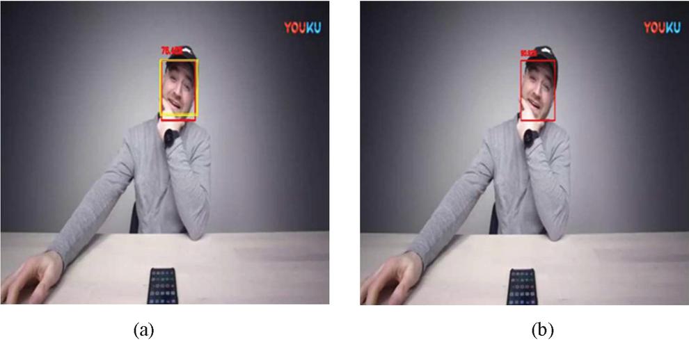
Figure 5 (a) Current frame detection result continuous frame tracking result; (b) Continuous frame tracking and detection fusion results.
According to the principle that the closer the tracking result is to the current frame, the more accurate the tracking result is in general. The confidence weight of the tracking result of the previous frame is set to a, the confidence weight of the tracking result of the first two frames is a, and so on for the tracking confidence weight of the first m frames. The best tracking position of the current frame is calculated by using the weighted average form consecutive frames, as shown in Equation (8).
| (8) |
Where is the four vertex coordinates of the tracking frame in the current frame, is the four vertex coordinates of the tracking frame in the previous i frames, and is the confidence weight of the tracking result in the previous i frames.
Finally, the confidence of the best tracking position is fused into the face detection result. The face detection confidence score is shown in Equation (9).
| (9) |
Where is the improved SSD face detection confidence of the i frame, is the calculated best tracking position confidence, and is the face detection confidence of the i frame. and are the weights of the detection and tracking results, respectively. This method can effectively reduce the missed detection due to face pose changes and occlusion.
4 Experimental Results
4.1 Datasets
In this paper, the validation set and FDDB dataset from the WiderFace dataset were used for the experiments, and the models were evaluated and analyzed using two evaluation methods: Average -Precision (AP) and ROC curve.
4.2 Experimental Configuration
This study uses PyTorch’s deep learning framework to change the SSD based network to ResNet18 to retrain the Rest-SSD face detection model. The Rest-SSD network model crops the input image to 300 300 size and initialises the network model parameters using Xavier; the initial learning rate of the network model is 0.0001, and the learning rate is 0.0001. When the number of training iterations reaches 80,000, the learning rate is modified to 0.00001. Thereafter the number of training iterations increases by 20,000, and the learning rate decreases by 1/10. The maximum number of iterations is 120,000, and the batch data size is 16.
4.3 Experimental Results
4.3.1 Average detection rate
In this paper, we use AP metrics to evaluate the trained Rest-SSD face detection model and the classical method VJ, the LDCF algorithm with better detection effect in non-deep learning, and the Faceness algorithm, MTCNN algorithm, HR algorithm, Face R-CNN algorithm, and SSH algorithm with better detection effect in current deep learning, and according to the number of faces within the picture, we can classify the WiderFace validation set into three difficulty test sets: easy, medium and hard. The empirical results are shown in Table 4.
Table 4 Experimental results comparison table
| Face | Simple Test | Medium Test | Difficult Test |
| Detection Methods | Set (AP) | Set (AP) | Set (AP) |
| VJ | 0.412 | 0.333 | 0.137 |
| LDCF | 0.797 | 0.772 | 0.564 |
| Faceness | 0.716 | 0.604 | 0.315 |
| MTCNN | 0.85 | 0.82 | 0.6 |
| HR | 0.923 | 0.910 | 0.819 |
| Face R-CNN | 0.930 | 0.918 | 0.831 |
| SSH | 0.927 | 0.915 | 0.844 |
| Rest-SSD | 0.937 | 0.921 | 0.834 |
4.3.2 Average operating efficiency
Based on the FPS metric as the object, the operational efficiency of the Rest-SSD face detection network was systematically evaluated and the results obtained are presented in Table 5. One thousand images were selected and fed into the model to be predicted, consuming a total of 21.7 s. The operational efficiency of Rest-SSD was calculated, and its value was 46 FPS, which far exceeds the values of some classical networks.
Table 5 Average operating efficiency comparison
| Face Detection Methods | Average Operating Efficiency (FPS) |
| Faceness | 20 |
| LDCF | 2.5 |
| MTCNN | 16 |
| Faster-RCNN | 3 |
| Face R-CNN | 7 |
| Face-Boxes | 20 |
| SFD | 36 |
| Rest-SSD | 46 |
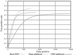
4.3.3 Comparative analysis of FDDB datasets
In this paper, the trained Rest-SSD face detection model and the AdaBoost algorithm, which has the best binary classification effect among the traditional face detection algorithms, are experimentally compared in the FDDB dataset and evaluated by plotting ROC curves. The experimental results are shown in Figure 6. As shown in this figure, the classification performance of the face detection algorithm of Rest-SSD is better than that of the traditional AdaBoost algorithm.
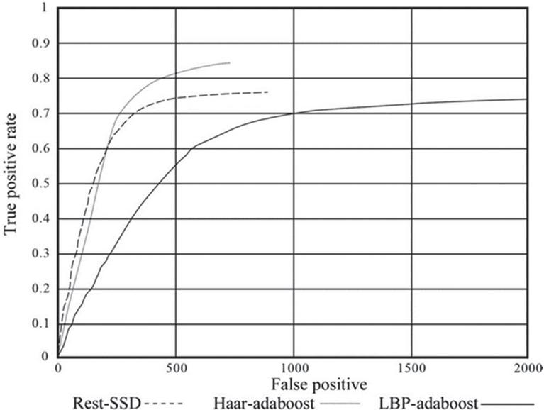
Figure 6 ROC comparison curve.
4.4 Face Detection Results of Fused Tracking Results
There are two kinds of target tracking algorithms: discriminant model tracking algorithm and generative model tracking algorithm. Among them, the latter refers to the establishment of a correlation model for the target region based on the current frame and the search for the region most similar to the model in the next frame, such as Kalman filtering, particle filtering and other tracking algorithms. The former is to extract the target and background information to train the classifier, separate the target from the background, and use the idea of classification to find the position most similar to the target. The biggest difference between them is that the classifier in discriminant tracking algorithm adopts machine learning and background information for training process, so the classifier can distinguish the target and background more accurately, so the discriminant method is generally better. In this study, the discriminant class tracking algorithm – Kernel Correlation Filter (KCF) tracking algorithm was used.
In the experiment, in order to avoid the tracking algorithm having errors causing too high confidence in the region without faces, the weights of the tracking results should be set reasonably. Through several tests, it is found that the weight k of the tracking algorithm and the weight k of the detection algorithm in the experiment are 0.5 and 1. In the experiment, because the tracking results of more than 5 consecutive frames have errors, this paper uses 5 consecutive frames for tracking, and the confidence weight of the previous frame tracking is set to 0.5, the confidence weight of the previous frame tracking is (0.5), and so on.
The experimental results are shown in Figure 7. Figure 7(a) shows the detection and tracking before the fusion tracking result, and only the tracking result, and Figure 7(b) shows the detection result after the fusion tracking, which effectively solves the situation that faces are not detected in the video due to pose change and semi-occlusion.
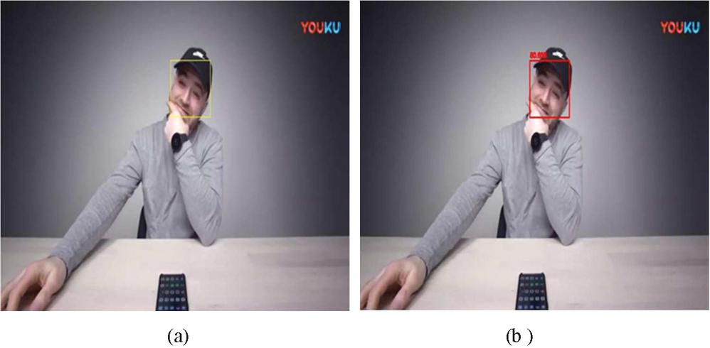
Figure 7 (a) Before fusion tracking Detection results; (b) Detection results after fusion tracking.
In this paper, the video face detection performance comparison test of RestNet-SSD face detection and fusion tracking results of video face detection is conducted using the video part video about face in aloveface video dataset, and the experimental results are shown in Table 6.
Table 6 Comparison table of experimental results
| Video | Video Frames | Rest-SSD Video | Fusion Tracking Results of Rest-SSD |
| Serial Number | with Faces | Face Detection | Video Face Detection |
| 1 | 294 frames | 182 frames | 193 frames |
| 2 | 230 frames | 114 frames | 189 frames |
| 3 | 699 frames | 335 frames | 405 frames |
| 4 | 496 frames | 296 frames | 367 frames |
| 5 | 465 frames | 407 frames | 431 frames |
| 6 | 525 frames | 453 frames | 483 frames |
| 7 | 1629 frames | 1356 frames | 1369 frames |
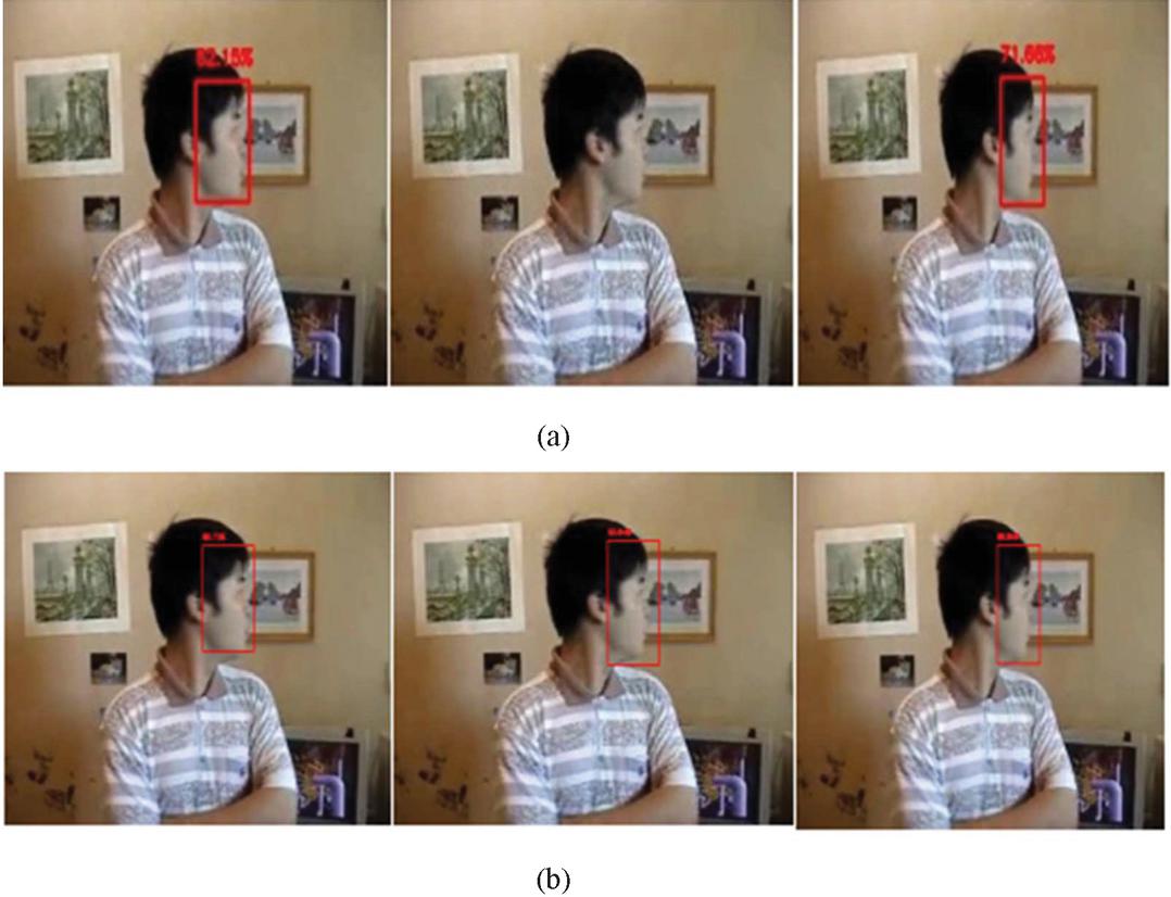
Figure 8 (a) Rest-SSD face detection results; (b) Face detection results with fused tracking results.
From experimental results, it can be learned that video face detection with fused tracking results increases the detection accuracy of Rest-SSD face detection to some extent. This is because when the confidence level of the face detection result is low, it will determine that no face is detected; however, when the tracking result occupies a certain weight, it will increase the confidence level of the face detection result, which will lead to a certain improvement in the accuracy of the detected face.
Figure 8 shows the results of face detection in the aloveface video dataset. Group (a) images are the results detected when target tracking is not introduced into the set. The face miss detection problem often occurs due to a variety of factors, where faces that can be detected in some frames are, however, given low confidence by the detection algorithm in other frames due to a variety of factors. The introduction of the target tracking algorithm yields the results shown in the images of groups (b). In this study, by introducing the target tracking algorithm, the connection between the front and back frames is enhanced, and the confidence level of the detection results is substantially improved, reducing the probability of missing detection problems.
5 Conclusions
In this paper, we study methods such as video face detection with deep learning related theories as the research background, and the work done is summarized as follows: an improved SSD face detection method is proposed, which uses ResNet residual network as the base network of SSD network model to train a Rest-SSD detection model for face detection. The base network in the neural network extracts features input to the prediction network for detection at different scales, while the network generates a score for each face in the prediction stage for each preset box, and finally a non-maximal suppression method is used to generate detection results. The experimental results show that the method improves the video face detection accuracy and is suitable for face detection in videos.
In addition, this paper illustrates the association between face detection and target tracking, and views the prediction generated by the target tracking algorithm as a temporal feature, and fuses the tracking results within the Rest-SSD face detection results to reduce the probability of the occurrence of the missed detection problem caused by face occlusion and pose change. Finally, an experimental approach is taken to verify whether target tracking can improve face detection accuracy. Experimental results show that by introducing the target tracking algorithm, the connection between the front and back frames is enhanced, the confidence of detection results is greatly improved, and the probability of missing detection is reduced.
References
[1] Ming-Hsuan, Y.; Kriegman, D.J.; Ahuja, N. Detecting faces in images: a survey. IEEE Transactions on Pattern Analysis and Machine Intelligence 2002, 24, 34–58, doi:10.1109/34.982883.
[2] Kuo, W.; Hariharan, B.; Malik, J. DeepBox: Learning Objectness with Convolutional Networks. In Proceedings of the 2015 IEEE International Conference on Computer Vision (ICCV), 7–13 Dec. 2015, 2015; pp. 2479–2487.
[3] Shi, Y.; Yu, X.; Sohn, K.; Chandraker, M.; Jain, A.K. Towards Universal Representation Learning for Deep Face Recognition. In Proceedings of the 2020 IEEE/CVF Conference on Computer Vision and Pattern Recognition (CVPR), 13–19 June 2020, 2020; pp. 6816–6825.
[4] Girshick, R.; Donahue, J.; Darrell, T.; Malik, J. Rich Feature Hierarchies for Accurate Object Detection and Semantic Segmentation. In Proceedings of the 2014 IEEE Conference on Computer Vision and Pattern Recognition, 23–28 June 2014, 2014; pp. 580–587.
[5] He, K.; Zhang, X.; Ren, S.; Sun, J. Spatial Pyramid Pooling in Deep Convolutional Networks for Visual Recognition. IEEE Transactions on Pattern Analysis and Machine Intelligence 2015, 37, 1904–1916, doi:10.1109/TPAMI.2015.2389824.
[6] Tang, J.; Mao, Y.; Wang, J.; Wang, L. Multi-task Enhanced Dam Crack Image Detection Based on Faster R-CNN. In Proceedings of the 2019 IEEE 4th International Conference on Image, Vision and Computing (ICIVC), 5–7 July 2019, 2019; pp. 336–340.
[7] Ren, S.; He, K.; Girshick, R.; Sun, J. Faster R-CNN: Towards Real-Time Object Detection with Region Proposal Networks. IEEE Transactions on Pattern Analysis and Machine Intelligence 2017, 39, 1137–1149, doi:10.1109/TPAMI.2016.2577031.
[8] Wu, W.; Yin, Y.; Wang, X.; Xu, D. Face Detection With Different Scales Based on Faster R-CNN. IEEE Transactions on Cybernetics 2019, 49, 4017–4028, doi:10.1109/TCYB.2018.2859482.
[9] Jing, S.; Hu, C.; Wang, C.; Zhou, G.; Yu, J. Vehicle Face Detection Based on Cascaded Convolutional Neural Networks. In Proceedings of the 2019 Chinese Automation Congress (CAC), 22–24 Nov. 2019, 2019; pp. 5149–5152.
[10] Zhang, K.; Zhang, Z.; Li, Z.; Qiao, Y. Joint Face Detection and Alignment Using Multitask Cascaded Convolutional Networks. IEEE Signal Processing Letters 2016, 23, 1499–1503, doi:10.1109/LSP.2016.2603342.
[11] Dang, K.; Sharma, S. Review and comparison of face detection algorithms. In Proceedings of the 2017 7th International Conference on Cloud Computing, Data Science & Engineering – Confluence, 12–13 Jan. 2017, 2017; pp. 629–633.
[12] Ranjan, R.; Sankaranarayanan, S.; Bansal, A.; Bodla, N.; Chen, J.; Patel, V.M.; Castillo, C.D.; Chellappa, R. Deep Learning for Understanding Faces: Machines May Be Just as Good, or Better, than Humans. IEEE Signal Processing Magazine 2018, 35, 66–83, doi:10.1109/MSP.2017.2764116.
[13] Jiao, L.; Zhang, R.; Liu, F.; Yang, S.; Hou, B.; Li, L.; Tang, X. New Generation Deep Learning for Video Object Detection: A Survey. IEEE Transactions on Neural Networks and Learning Systems 2021, 1–21, doi:10.1109/TNNLS.2021.3053249.
[14] Redmon, J.; Divvala, S.; Girshick, R.; Farhadi, A. You Only Look Once: Unified, Real-Time Object Detection. In Proceedings of the 2016 IEEE Conference on Computer Vision and Pattern Recognition (CVPR), 27–30 June 2016, 2016; pp. 779–788.
[15] Chengcheng, N.; Huajun, Z.; Yan, S.; Jinhui, T. Inception Single Shot MultiBox Detector for object detection. In Proceedings of the 2017 IEEE International Conference on Multimedia & Expo Workshops (ICMEW), 10–14 July 2017, 2017; pp. 549–554.
[16] Hua, W.; Tong, Q. Research on Face Expression Detection Based on Improved Faster R-CNN. In Proceedings of the 2020 IEEE International Conference on Artificial Intelligence and Computer Applications (ICAICA), 27–29 June 2020, 2020; pp. 1189–1193.
[17] Lavinia, Y.; Vo, H.H.; Verma, A. Fusion Based Deep CNN for Improved Large-Scale Image Action Recognition. In Proceedings of the 2016 IEEE International Symposium on Multimedia (ISM), 11–13 Dec. 2016, 2016; pp. 609–614.
[18] Kuo, W.; Hariharan, B.; Malik, J. DeepBox: Learning Objectness with Convolutional Networks. In Proceedings of the 2015 IEEE International Conference on Computer Vision (ICCV), 7–13 Dec. 2015, 2015; pp. 2479–2487.
[19] Liu W, Anguelov D, Erhan D, et al. Ssd: Single shot multibox detector[C]. European conference on computer vision. Springer, Cham, 2016: 21–37.
[20] Yang, S.; Luo, P.; Loy, C.C.; Tang, X. WIDER FACE: A Face Detection Benchmark. In Proceedings of the 2016 IEEE Conference on Computer Vision and Pattern Recognition (CVPR), 27–30 June 2016, 2016; pp. 5525–5533.
[21] Fu, J.; Alvar, S.R.; Bajic, I.; Vaughan, R. FDDB-360: Face Detection in 360-Degree Fisheye Images. In Proceedings of the 2019 IEEE Conference on Multimedia Information Processing and Retrieval (MIPR), 28–30 March 2019, 2019; pp. 15–19.
Biographies

Yilin Liu received her bachelor’s degree in Electronic information Engineering from Huaiyin Institute of Technology in 2018. She is currently studying intelligent science and technology at Tianjin Normal University and will receive her master’s degree in 2022. Her research interests include face recognition, facial expression recognition and target detection.

Ruian Liu, Professor, received a Ph.D. degree in Precision Instrument and Opto-electronics Engineering from Tianjin University. He is currently Head of School of Electronics in the College of Electronic and Communication Engineering at Tianjin Normal University. His current research interests include image processing, deep learning and artificial intelligence, etc.

Shengxiong Wang received his bachelor’s degree of Electronic Information Engineering from Tianjin University of Science and Technology in 2020. He is currently studying for a master’s degree of Information and Communication Engineering in Tianjin Normal University and will receive his master’s degree in 2023. His research interests are computer vision, object detection and image processing.
Da Yan received a Bachelor of engineering degree from Yantai University, Yantai City, Shandong Province, majoring in communication engineering. Now studying in Tianjin Normal University, majoring in intelligent science and technology. His research fields include the solution of occlusion in pedestrian re recognition and pedestrian re recognition based on local features.

Bo Peng received her bachelor’s degree in Communication Engineering from Tianjin University of Commerce in 2019. She is currently studying Electronic Message at Tianjin Normal University and will receive her master’s degree in 2022. Her research interests include image enhancement and image denoising.

Tong Zhang is studying for a master’s degree in electronic information from Tianjin Normal University in China. His research fields include face recognition and small target high-precision detection in complex environment.
Journal of Web Engineering, Vol. 21_2, 545–568.
doi: 10.13052/jwe1540-9589.21218
© 2022 River Publishers