Two-stage Detection of Semantic Redundancies in RDF Data
Yiming Chen, Daiyi Li†, Li Yan and Zongmin Ma*
Nanjing University of Aeronautics and Astronautics, China
E-mail: zongminma@nuaa.edu.cn
*Corresponding Author
†Co-first Author
Received 20 March 2022; Accepted 11 January 2023; Publication 13 March 2023
Abstract
With the enrichment of the RDF (resource description framework), integrating diverse data sources may result in RDF data duplication. Failure to effectively detect the duplicates brings redundancies into the integrated RDF datasets. This not only increases unnecessarily the size of the datasets, but also reduces the dataset quality. Traditionally a similarity calculation is applied to detect if a pair of candidates contains duplicates. For massive RDF data, a simple similarity calculation may lead to extremely low efficiency. To detect duplicates in the massive RDF data, in this paper we propose a detection approach based on RDF data clustering and similarity measurements. We first propose a clustering method based on locality sensitive hashing (LSH), which can efficiently select candidate pairs in RDF data. Then, a similarity calculation is performed on the selected candidate pairs. We finally obtain the duplicate candidates. We show through experiments that our approach can quickly extract the duplicate candidates in RDF datasets. Our approach had the highest F score and time performance in the OAEI (Ontology Alignment Evaluation Initiative) 2019 competition.
Keywords: RDF redundancy, duplicate data, RDF similarity, candidate selection.
1 Introduction
The development and standardization of the Semantic Web have resulted in an unprecedented volume of data being published on the Web as linked data [1]. Linked data are used for publishing structured data using vocabularies like schema.org, which can be connected and interpreted by machines. Linked data uses URIs and an RDF to connect pieces of data, information, and knowledge on the Web.
The resource description framework (RDF) is a logical model that describes data in the form of triples. Each triple contains a subject, a predicate, and an object. The subject corresponds to the resource being described, the predicate corresponds to the attribute of the resource, and the object corresponds to the value of the attribute. A set of RDF triples can be regarded as a directed graph, in which subjects and objects are the nodes, and predicates label the edges from the subject nodes to the object nodes.
However, it should be noted that due to the diversity of data sources, linked data that cover different domains are usually generated independently, distributed in many locations, and are heterogeneous. There are likely duplicates in the linked data. That is, in the link data, different URIs may point to the same entity in the real world. For example, a person may have different URIs in many database systems, but such URIs represent the same person. It means that if RDF data are generated from such datasets, the same entities may occur multiple times. Here the repeatedly introduced information are used to describe this entity.
The duplicate data may lead to many duplicate search results or incorrect statistical information about Web entities [2]. After storing these duplicates, data redundancies are introduced, and this increases unnecessarily the data set size. In particular, RDF data redundancies affect a wide range of applications, including query, data publishing, and ontology reasoning. Low data quality will not only increase the overhead cost of downstream applications, but also affect performance and cause more complex problems. A better understanding of data redundancies in linked data can help us know more and facilitate more effective and efficient exploitations on the linked data [3].
The traditional methods to solve the problem of data duplication are to calculate similarities of resources. By calculating the similarity score of two resources, duplication can be judged. In the context of link data, current methods for detecting link data duplication face two major problems. The first one is the issue of their scalability and the second one is the issue of their coverage. The current approaches for detecting RDF replication can only handle such a task for small data volume and have low precision. A single dataset of linked data may have millions of instances (e.g., DBpedia and Freebase). It is clear that expensive matching for one-to-one comparisons is time-consuming and not effective [15], and such brute-force approaches that compare every pair of instances cannot scale well [17]. In addition, many existing methods of link data duplication detection are proposed for one of the application fields with the expert experience. Their accuracy may be higher than some common approaches, but their development requires a lot of manpower and they cannot be performed well in multi-domain datasets.
With the rapid development and wide applications of linked data, we are faced with how to find duplicates in large and multi-domain RDF datasets effectively and efficiently, which is a challenging task. In this paper, we concentrate on finding duplicates in large and multi-domain RDF datasets. The main contributions of this paper are as follows:
(1) We propose a candidate selection approach for screening candidates. Our approach is based on local sensitive hashing (LSH) to select approximately similar candidates in RDF dataset. It can effectively solve the problem of the large time complexity caused by the linear search of massive RDF data and has excellent time performance. The experimental results show that our approach has the improved accuracy and F score.
(2) We propose an approach called RDFsim to calculate the similarity of RDF resources. Our approach is domain-independent and applies the pruning technology to improve the speed of calculating the resource similarities. The experimental results show that our approach can well calculate the similarity of RDF data in different fields.
The rest of the paper is organized as follows. In Section 2, we discuss the related work. In Section 3, we investigate the candidate selection algorithm. In Section 4, we propose the similarity algorithm of RDF resources. We show our evaluation results in Section 5 and conclude and describe future work in Section 6.
2 Related Work
2.1 RDF Redundancy
Data redundancy traditionally means that the same piece of data is stored in multiple places in a database [3]. In terms of RDF data, RDF data redundancy is identified into three categories, which are syntactic redundancy, semantic redundancy, and symbolic redundancy [4].
Symbol redundancy involves unnecessary repetition of symbols in RDF datasets. The basic idea of redundancy elimination is to encode each element (e.g., URI, blank node, and text) of the RDF graph with the corresponding integer identifier (ID), where the identifiers are stored in the dictionary. Syntactic redundancy depends both on the serialization of RDF graph and the underlying graph structure. With NTriples, the simplest RDF syntax, all triples are written line by line to serialize the RDF subgraph. Suppose that we have n RDF triples with the same subject. Then, the same subject repeatedly appears n times in the generated file. Semantic redundancy means that, if certain RDF triples can be deleted without any change in their semantics, the redundancy generated by these triples is semantic redundancy.
The above three categories of RDF data redundancy are summarized in [3], where symbolic redundancy and syntactic redundancy are classified as serialization level of redundancy, and semantic redundancy is classified as data model level of redundancy. At the serialization level of redundancy, redundant data is represented as a sequence of bits. Given a fix set of triples, one serialization is said to be more redundant than the other if it uses more bits than its counterpart. It is a major research issue in the compression field and is beyond the scope of this article. At the data model level of redundancy, the size of data can be calculated by the number of triples. Hence, at this level, the data redundancy exists if less triples can be used to represent the same semantic meanings of the original data. The focus of this paper is on the semantic redundancy. Determining and eliminating semantic redundancy is more conducive to data cleaning.
There have been some efforts in eliminating RDF semantic redundancy based on rule-based reasoning [6–8]. The core idea of these methods is to make reasoning with the existing rules, and then the semantic information inferred can be regarded as redundant information, which hereby need to be eliminatedAs stated in [6], for example, there is a rule in OWL2RL: if (?p, rdfs:domain, ?c) (?x, ?p, ?y), then (?x, rdf:type, ?c). Again, in the FOAF ontology, we have: (foaf:lastName, rdfs:domain, foaf:person). Then, for any subject s with foaf:lastName attribute, (s, rdf:type, foaf:person) is regarded as redundant. The elimination of such semantic redundancies can indeed reduce the number of triples without missing semantics, but this may not be conducive to practical applications. These redundancies are often helpful for our applications. The semantic information deleted by this method may lead to a large number of query rewrites, which is not conducive to the use of data. Suppose that, for example, we would query all triples that have the rdf:type attribute and the attribute value is foaf:person. At this point, removing the semantic redundancy triples in the above example must cause a lot of query rewriting. And the query processing has to write the deleted triples back to the RDF dataset first. This actually increases the burden on the query processing.
We argue that the main source of RDF semantic redundancy should be some duplicate resources or the semantic information carried by these duplicate resources. In the Semantic Web, owl:sameas is used to describe two equivalent entities. These two entities may have different URIs but point to the same real-world entity. The process of producing links (e.g., owl:sameAs) or interlinking has been studied in the community of natural language processing as the entity coreference and entity resolution problems as well as in the community of databases as the deduplication and record linkage problems [17].
2.2 Similarity of Duplicate RDF Resources
Detecting duplicate RDF resources is the process of identifying the resources with the same semantics and different identifiers. The typical approach for detecting duplicate resource depends on measuring a degree of “similarity” between pairs of objects using certain metrics. With such a similarity degree, we can decide if a pair or groups of pairs are mutually duplicate. This is often done by using the strategies based on similarity threshold, classification, or clustering methods [9].
It is a common way to use a similarity measure in identifying duplicate resources. Its core is to construct the context of all resources, compare this context in the dataset, and finally find if there are resource pairs with similar contexts. If the similarity is higher than the given threshold, one of the resources in the resource pair is considered redundant. At present, many approaches for RDF data similarity measure have been proposed. Among them, some of similarity measure approaches (e.g., [10–12]) are mostly used in isomorphic datasets and mainly applied for approximate search, QA (question–answer) systems and so on, rather than duplicate resource identification.
K-Radius subgraph comparison [2] performs a similarity calculation by constructing k-order subgraphs, but it does not consider the discriminability of triples (i.e., the weight of similarity measures in different contexts) and its accuracy is low. In [15], RDF datasets are detected by using Hadoop and MapReduce. Compared with other methods, the method proposed in [15] is fast in time, but it is too simple and may lead to low accuracy. The similarity approach RiMOM in [14], by manually assigning attribute weights, can effectively solve the problem of the weight of triples in the similarity calculation, but in the context of big data, the time cost of this method is too high to implement it. In [13], a domain-independent entity co-referencing algorithm is proposed, which can better solve this problem by analyzing the classification capabilities of triples to set weights, but the structure of the context representation is too complicated, and the time cost is high also. In addition, this method does not perform very well in terms of scalability.
Candidate selection is a key part of the time efficiency and scalability of redundant detection algorithms. The goal of candidate selection is to identify the entities that are worth making comparison. In [16], a supervised learning method is proposed to learn a candidate selection technique. However, the supervised methods require sufficient training data, which may not always be available. In [17], an unsupervised learning method is used to learn the key value to build an index, which is suitable for multiple types of data. However, the space cost and time cost of its indexing method are too large, and the number of candidate pairs that can be reduced is also limited.
To find redundant RDF data, we propose a two-step approach. In the first step, we deal with the issue of scalability, which is not handled well for massive RDF data in most current work. We only select the same RDF resource pairs as candidates. This can greatly narrow the range of redundant detection. In the second step, we introduce a metric for specifying redundant resources.
3 Candidate Selection
Calculating the similarities of all resources in massive datasets is time-consuming due to many meaningless calculations. For example, some resource pairs are obviously different, and they can be filtered out in advance through simple and low-cost methods to avoid the complex similarity calculation. Candidate selection is the process of efficiently selecting instance pairs that possibly match each other by comparing the part of their context information only [17]. When the dimensions of users and items are in the tens of millions or even higher, the similarities are directly calculated, and the computational cost is extremely high even if it is possible to use large-scale computing clusters. To this end, it is necessary to use an approximate method, which can improve the calculation efficiency by sacrificing the precision. MinHashing and locality sensitive hashing (LSH) can be used to improve the computational efficiency. In this paper, our candidate selection is based on the local sensitive hash algorithm. We first select a set of keys with the best discrimination in the dataset, and then construct the text information of each resource based on these keys. Finally, a local sensitive hash algorithm is used to cluster resources with similar text information to generate several sets of candidates.
3.1 RDF Resource Representation
Traditionally the LSH is mainly used for document clustering, where document contents are divided and regarded as the features of document. In the context of RDF data, however, RDF resources are composed of graph data. We have to express RDF data in a form that can be used by the LSH algorithm. In the RDF graph, the node that is directly connected to the resource node has the closest relationship to the resource node. We choose the triplet with subject or object of resource as resource information. However, for large-scale RDF data, the number of resource features is too large, and a large part of the features does not actually contribute to the similarity calculation. Therefor we need to filter out these useless features.
A stronger classification ability of the triplet means a greater contribution to the similarity calculation. Here the classification ability of the triplet depends on the classification ability of the predicate in the triplet. For this reason, we use an unsupervised method to learn a set of predicates (candidate selection keys), which has a great contribution to similarity and big coverage in building the features of RDF resources. Our goal is to learn a set of predicates (i.e., candidate selection keys) that are sufficiently distinguishable so that most instances in a given dataset use at least one learned predicate. Algorithm 1 presents the process for learning the candidate selection key.
Algorithm 1 LearnKey(G, C, , )
1: RDF graph G, classes C in G, and parameters and for the lower limits of discrimination and coverage.
2: key_set.
3: key_set all predicates G
4: Ic {, rdf:type, C}
5: satisfied false
6: if not satisfied: then
7: for key in key_set do
8: dis discriminability(key, Ic, G)
9: if dis then
10: key_set key_set key
11: else
12: cov coverage(key, Ic, g)
13: FL (2*dis*cov) / (dis cov)
14: if FL then
15: satisfied True
16: learn_key[key] FL
17: if not satisfied then
18: print(‘ and values are set too high’)
19: return key_set
This algorithm is to obtain the predicates that satisfy the parameters \alpha and \beta under a certain categories C. The algorithm first constructs a set of all instances of type C, denoted IC, then searches for all predicates in the RDF dataset G, and also selects the predicates with the subject from IC, where the discriminability is greater than \beta and the F score is greater than \alpha, and finally adds them in to the result set. Here sufficient discriminability and coverage can efficiently select similar pairs and reduce election of non-matching pairs. We define discriminability and coverage in Equations (1) and (2), respectively.
| (1) | ||
| (2) |
Here i and o represent the subject and object of the triple, respectively.
With the candidate selection keys, we can build the resource features. First, we build the feature triple set of resource with Equation (3).
| (3) |
Here G is an RDF graph, r is the resource, and K is candidate selection keys. We use the k-shingles method proposed in [18], which is an effective way to represent document as sets, to represent the object in every feature triple. In addition, for the k-shingles set formed by each triplet, we also need to add a predicate before the elements in the k-shingles set. Let us look at an example.
Example 1. For Feature(K, G, r) {r, dblp:fullname, Chris Bosh}, let k 5. Then we have the features of the resource: {dblp:fullname/Chris, db lp:fullname/hrisB, dblp:fullname/risBo, dblp:fullname/isBos, dblp:fullname/ eBosh}.
3.2 Locality-sensitive Hashing for RDF Data
The locality sensitive hashing (LSH) algorithm is one of the most popular algorithms of approximate nearest neighbor search. LSH has a solid theoretical foundation and can perform well in high-dimensional data spaces. Its main function is to dig out similar data from a massive dataset and can be specifically applied to text similarity detection, Web search, and so on.
With the feature representation of RDF resources, we now use the LSH algorithm to obtain RDF data clusters, where each cluster has a similar feature. First, we obtain the feature sets of all resources and then establish the characteristic matrix representation of these feature sets. Finally, we use the “MinHash” algorithm in [18] to reduce the dimensionality of the characteristic matrix and build the signature matrix. The so-called “MinHash” refers to randomly shuffling the rows of the characteristic matrix, taking the row number of the first non-zero element in each column as the “MinHash Value” of the resource, and performing n times Scrambling to generate n “MinHash Value”, which constitutes the “MinHash Signature” vector of the resource. The dimension of the signature vector is usually much lower than the number of elements in the feature set, and it is equivalent to dimensionality reduction. We apply the dimensionality reduction feature vectors to measure the similarity between users.
It should be noted that MinHash can reduces the complexity of document similarity comparison, but the number of comparisons may still be quite large even if the number of documents is small. For our goal of calculating the similarity between any two resources, we can use a cluster to calculate the similarity. But, in general, we only want to know “the similarity of some very similar pairs”. So, we only need to pay attention to those “more likely similar pairs” and ignore the remaining pairs. This is the core idea of LSH. LSH divides the Signature matrix into b bands, which consist of r rows and each is based on the signature matrix obtained by MinHashing, as shown in Figure 1.
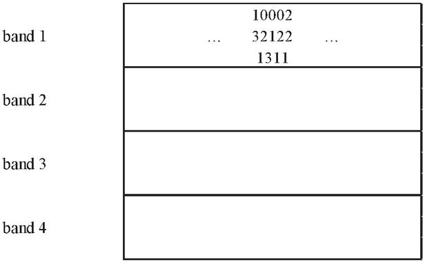
Figure 1 Dividing a signature matrix into four bands of three rows per band.
Our basic idea here is: if one or more bands of two vectors are the same, the resources represented by these two vectors may have a higher similarity; if there are more of the same bands, the likelihood of their similarity is higher. Therefore, the method of LSH is to hash the signature vector of each resource on each band separately, and the resources that are allocated to the same bucket on any band should be the candidates for similar resources. In this way, we only need to calculate the similarity of all candidate resources to find the similar resource group of each resource.
Suppose that we use b bands of r rows and also suppose that a particular pair of documents have Jaccard similarity s. The probability that the signatures agree in all the rows of at least one band and thereby become a candidate pair is . As long as we control the size of b and r, we can set the similarity as a candidate pair as much as possible.
We summarize our processing with LSH as three main steps: looking for a candidate pair as candidate similar resources, calculating the similarity between them, and determining the true similar resources. We present our processing in detail as follows.
• Perform word segmentation or k-shingles on the resource feature set to construct the characteristic matrix (rows are words and columns are resources).
• Choose a dimension n (the number of hash functions), calculating n rows of MinHash on the characteristic matrix, and constructing a MinHash signature matrix.
• Selecting the number of blocks b and the number of block rows r (b*r n), and setting a threshold t\approx(1/b)/1/r.
• Using LSH for the signature matrix, dividing the resources into buckets, and constructing a candidate pair.
• Examining each candidate pair’s signatures and determining if the fraction of components is at least t.
• For the candidate pairs with similar signatures, checking their similarity to prove if they are duplicate resources.
4 RDF Resource Similarity Calculation
For the selected candidates, in this section we propose an approach named RDFSim, which is used to calculate the similarity between RDF resources. When the similarity value of two RDF resources is higher than the given threshold, two resources are regarded as a pair of duplicate resources.
4.1 Context Representation for RDF Resources
RDF data model with triples can be regarded as directed graphs, in which subjects and objects are the vertices and predicates are the edges from subject vertices to object vertices. Therefore, RDF datasets are usually represented as labelled directed graphs. Then the similarity of RDF resources is calculated based on the context of the resources. Here the context refers to the graph that is formed with the nodes and edges connected to the target node. The context contains the adjacency graph linked to the resource and it is so an important basis of describing the resources in the datasets.
Definition 1 (Path): In an RDF graph, predicates are represented by edges, and subjects and objects are represented by vertices. Then a path in the RDF graph is represented as a sequence as follows.
| (4) |
Here i is an instance, node[i] (i 0) is any other expanded node from the RDF graph, and predicate[i] is a predicate that connects two nodes in a path.
The depth of a path is the number of predicates in this path. The path direction represents the positive and negative of a predicate in the path. For a predicate, if its connected left and right are respectively a subject and an object, we say the direction of this predicate is positive and have (subject, predicate, object); if its connected left and right are respectively an object and a subject, we say the direction of this predicate is negative and have (object, predicate, subject).
The idea of obtaining the context information of a target RDF resource is to find a subgraph with this resource as the center and a specified distance as the radius. This subgraph represents the context of the target node. For the purpose of using such a subgraph to calculate the similarity, we construct a set of paths to represent the subgraph. We treat the subgraph as an undirected graph and then construct a set of paths from the target node to other nodes with a length of a specified distance. After the construction is completed, the direction of edge in the subgraph is added to the path.
Starting from the target node, we search in the graph for the nodes, which are directly linked to the target node and each linked node forms a path. The last node of each path is treated as a new target node. We continue to expand the path according to the expansion method of the previous step until the last node type is a Literal or a required depth of the path is reached. We describe the context representation of RDF resource in Algorithm 2.
Algorithm 2 GetContext(i, G, limit_depth)
1: RDF graph G, the upper limit limit_depth of path depth, and resource i in G.
2: path.
3: path i
4: expansion_set {path}
5: paths { }
6: for path in expansion_set do
7: last path[1]
8: pre_p path[2]
9: if type(last) == Literal or depth(path) == limit_depth then
10: paths union(paths, path)
11: else if depth(path) limit_depth then
12: for all t = last, p, o in G do
13: if not (p.v == pre_p.v and p.dirct != pre_p.dirct) then
14: new_path path.append(p,o)
15: expansion_set.add(new_path)
16: for all t s, p, last in G do
17: if not (p.v == pre_p.v and p.dirct != pre_p.dirct) then
18: new_path path.append(p-,s)
19: expansion_set.add(new_path)
20: expansion_set.remove(path)
21: return path
The path constructed with this algorithm can represent the context of the given target node very well. More importantly, with the constructed path, the comparison calculation between two paths replaces the complicated comparison between two graphs. We present an example to illustrate our idea.
Example 2. Suppose that we have an URI node i and its context representation is given in Figure 2. We set that the expansion depth is 2. Then the semantic information of i should be composed of 5 paths: (node, p, node), (node, p, node), (node, p, node, p, node), (node, p, node, p, node), and (node, p, node, p, node).
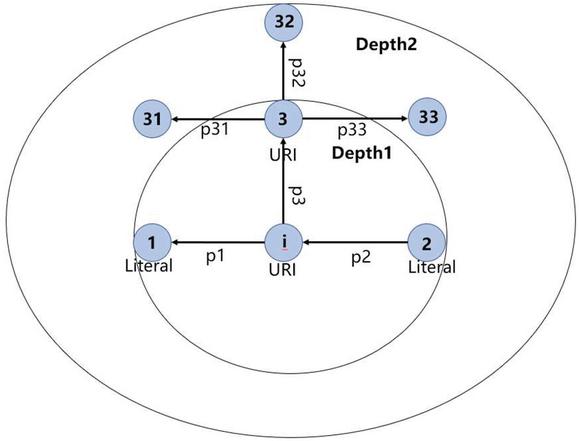
Figure 2 Semantic information for node i.
With the context representation of RDF resources, we can further calculate the similarities among RDF resources and then find out possible data redundancies.
4.2 Weight of Path in RDF Graph
It was shown in Section 4.1 that, for a resource node, its set of paths constitutes its context information. To calculate the similarity, it is necessary to know the weight of each path in the similarity calculation. Before we discuss the weight of path, we first analyze the weight of the triples contained in the given path.
As we may know, triples with strong classification ability should have greater weight, which can distinguish similar nodes well. Therefore, triple weights should be positively related to the classification ability of predicates. We calculate the triple weights mainly through the classification ability of triple predicates. As for a predicate, the more diverse value set it has, the stronger classification it is. The classification ability of triple predicates can be calculated with Equations (5) and (6) as follows.
| (5) |
Here Per represents a percentage for predicate .
We know that a predicate in the path has a direction. While we calculate the classification ability of the predicate in the path, different direction should use different calculation. Let the direction of predicate p be positive. Then the classification ability of p is calculated by dividing the size of p’s distinct object value set by p’s number of occurrences in the entire dataset. If the direction of p is negative, the classification ability of p is calculated by dividing the size of p’s distinct subject value set by p’s number of occurrences in the entire dataset.
Per is used to denote the largest percentage value over all predicates. On this basis, we normalize such values with Equation (3) so that the most discriminating predicate has a classification ability of 1.
| (6) |
Here “CS” represents the classification ability of the predicate.
For each node, we introduce a parameter, called factor, to indicate how important a node is with respect to its father node. After generating the context information of the target node, we believe that the nodes with a large distance from the target node should be less important to the target node; the nodes with a small distance from the target node should be important to the target node. Therefore, we evaluate the importance of a node based on its distance from the target node. At the same time, we also consider the number of branches of nodes in the RDF graph. The importance of a node can be calculated with Equation (7) as follows.
| (7) |
Here Im represents the node importance. For node node, its importance is calculated by dividing the importance of node’s parent node by the number of branches of node’s parent node. For the root node, its Im is equal to 1.
Example 3. We use the nodes given in Figure 2 to illustrate the calculation process of Im. We have the following calculation process.
Based on the analysis above, the triple weights are positively related to the classification ability of triple predicates. In addition, the triple importance for the context information of the target node should be equivalent to the importance of the node pointed to by the direction of the predicate in the triple. For example, if the predicate direction in the triple is positive, the importance of the triple is equivalent to the importance of the object in the triple, and vice versa is equivalent to the importance of the subject in the triple. We define Equation (8) to calculate the weight of triples.
| (8) |
Here W represents the triple weight. When the predicate direction is positive, we use Equation (8) to calculate the triple weight. If the predicate direction is negative, we use Equation (9) to calculate the triple weight.
As shown in Section 4.1, the context information of a node is composed of a set of paths. With the weights of the triples contained in the path, now we can calculate the path weight with Equation (9) as follows.
| (9) |
Here triple represents the triple formed by predicate.
Example 4. Suppose that we calculate the weight of path (node, p, node, p, node) in Figure 2. We have
The weight of the path is discussed in this section. In the next section, we use the path weight to calculate the semantic similarity between two resources in RDF graph.
4.3 Similarity Calculation
With the context of the RDF resource node and the weight of the path contained in the context information, we can calculate the similarity of resources to detect possible redundant RDF data. We present Algorithm 3 to complete this processing. Let uri1 and uri2 be two resources for the calculation of similarity. We first obtain their context information representation, which are represented by paths1 and paths2, respectively. Then, for each path (say, path1) in paths1, we further identify the following situations.
(1) The last element of path1 has the type of literal. At this point, we search in paths2 for all possible paths (say, such a path path2) that can be compared with path1. We calculate the similarity between path1 and path2, which is carried out by calculating the text similarity between their last elements. From all the similarities, we finally select one with the highest similarity, where the corresponding path2 is regarded as a match with path1. We add the similarity score of the matching item to path_score and calculate the weight of the two matched paths, which are added to path_weight.
(2) The last element of path1 has the type of URI. Then we search in paths2 for a possible path (say, path2) that can be compared with path1. We compare if the last element of path2 is the same as the last element of path1. If they are the same, path2 with the same last element is regarded as a match for path1. We add the similarity score of the matching item to path_score and calculate the weight of the two matched paths, which are added to path_weight. Finally, total_score is equal to the sum of the similarities of all matching pairs multiplied by the corresponding weights.
Algorithm 3 GetSim(uri1, uri2, G, limit_depth)
1: G is an RDF garph. limit_depth is the upper limit of path depth, uri1 and uri2 are two resources in G.
2: total_score 0
3: total_weight 0
4: paths1 Get_context(G, limit_depth, uri1)
5: paths2 Get_context(G, limit_depth, uri2)
6: for path1 in paths1 do
7: path_score 0
8: path_weight 0
9: if type(path1[1]) == Literal then
10: for path2 in paths2 do
11: if PathComparable(path1, path2) then
12: if Sim(path1[1], path2[1]) path_score then
13: path_score Sim(path1[1], path2[1])
14: path_weight (W(path1) W(path2))/2
15: if type(path1[-1]) == URI then
16: for path2 in paths2 do
17: if PathComparable(path1, path2) then
18: if path1[1] == path2[1] then
19: path_score 1
20: path_weight (W(path1) W(path2))/2
21: total_score total_score path_score * path_weight
22: total_weight total_weight path_weight
23: sim total_score / total_weight
24: return sim
In Algorithm 3, the PathCompareable function is used to mean if two paths can be compared and calculated for similarity. Two paths are considered to be comparable only when these two paths have the same depth and the predicates at the corresponding positions in the paths are comparable. The comparability of predicates means that two predicates have the same value and the same direction. If two predicates have different values, but one predicate is the ancestor of other predicate in the ontology model, the two predicates are also considered to be comparable. In Algorithm 3, the Sim function is used to calculate a text similarity. Here we use character-level n-gram similarity measure in calculating text similarity.
5 Performance Evaluation
This section evaluates our approach with several RDF datasets that are from several different fields and have different sizes. We compare our approach with several existing approaches to prove that our approach performs better over these RDF datasets.
5.1 Experimental Setting
We collected RDF data from the instance matching (IM) under the ontology alignment evaluation initiative (OAEI) platform. The OAEI is a coordinated international initiative to forge this consensus. The goals of the OAEI are to assess strengths and weaknesses of alignment/matching systems and help improving the work on ontology alignment/matching. The instance matching track aims at evaluating the performance of matching tools when the goal is to detect the degree of similarity between pairs of instances expressed in the form of OWL ABox. The task goal is to produce a set of mappings between the pairs of matching instances that are found to refer to the same real-world entity.
We constructed four datasets from IM@OAEI (2010) and IM@OAEI (2019), which have three types: Person, Restaurant and Creative Work. For the type of Creative Work, we collected two datasets with a small size and large size, respectively. We describe the details of these four RDF datasets in Table 1.
Dataset Person is a synthetic dataset, where the records with coreference are generated by modifying the original records. Dataset Restaurant is a real-world dataset, which is applied to match the instances describing restaurants from Fodors (331 instances) to Zagat (533 instances) with 112 duplicates. Dataset Creative Work contains ontology instances described through 22 classes, 31 DatatypeProperty and 85 ObjectProperty properties.
Table 1 Details of four RDF datasets
| Dataset | Number of Triples | Number of Instances | Number of Duplicates |
| Person | 16001 | 1000 | 500 |
| Restaurant | 10380 | 865 | 112 |
| Creative Work(small) | 22427 | 699 | 299 |
| Creative Work(large) | 97457 | 3519 | 1511 |
5.2 Evaluation Measures
To evaluate the performance of our proposed approach, we use three standard measures, which are precision, recall, and F score, and are computed in Equations (10), (11) and (12), respectively.
| (10) | ||
| (11) | ||
| (12) |
We downloaded the groundtruth of each dataset from the OAEI platform. The groundtruth can provide us with all duplicates in the datasets through owl:sameas. The correct matching duplicates in the above equations are obtained by searching groundtruth. Our experiments were implemented on Python 3.6 and used the rdflib package to process RDF data. All experiments were performed on a Window10 system running 2.90 GHz Intel i-7 processor and 8GB of memory.
5.3 Evaluation on OAEI@2019
To further demonstrate the capability of our approach in duplicates detection, we compared our approach with several approaches that are participated in the OAEI@2019 Campaign (Ontology Alignment Evaluation Initiative 2019) on the SPIMBENCH benchmark. This benchmark was designed for ontology instance matching, which consists of two tasks: SANDBOX and MAINBOX. The descriptions of these two tasks are similar, in which the SANDBOX contains a small dataset and the MAINBOX contains a large dataset.
The approaches participated in the competition mainly include AML [19], Lily [20], FTRL-IM [21], and LogMap [22]. Our approach is composed of LSH-based Candidates Selection and RDFSim algorithm for computing resource pair similarity. To form a comparison, we also selected the Candidates Selection Histsim [18] and matched it with RDFsim for our experiment. Histsim is a key reference in our research process and has been performed well in comparison with many other approaches.
Table 2 SANDBOX results in OAEI@2019
| SANDBOX (about 380 instances and about 20000 triples) | ||||||
| AML | Lily | FTRL-IM | LogMap | HistSimRDFsim | LSHRDFSim | |
| Fmeasure | 0.8645161 | 0.9185868 | 0.9214176 | 0.8413284 | 0.9424920 | 0.9566724 |
| Precision | 0.8348910 | 0.8494318 | 0.8542857 | 0.9382716 | 0.9021407 | 0.9928058 |
| Recall | 0.8963211 | 1.0000000 | 1.0000000 | 0.7625418 | 0.9866221 | 0.9230769 |
| Time performance | 6223 | 2032 | 1474 | 6919 | 249 | 110 |
The experimental results in Tables 2 and 3 show that our approach has excellent performance both in the SANDBOX and MAINBOX datasets. Our approach has the highest F score, precision and time performance in the experiments over both datasets.
Table 3 Results of MAINBOX in OAEI@2019
| MAINBOX (about 1800 instances and about 100000 triples) | ||||||
| AML | Lily | FTRL-IM | LogMap | HistSimRDFsim | LSHRDFSim | |
| Fmeasure | 0.8604576 | 0.9216225 | 0.9214788 | 0.7905605 | 0.9237233 | 0.9315938 |
| Precision | 0.8385678 | 0.8546380 | 0.8558456 | 0.8925895 | 0.9027164 | 0.9969811 |
| Recall | 0.8835209 | 1.0000000 | 0.9980146 | 0.7094639 | 0.9457313 | 0.8742555 |
| Time performance | 39515 | 3667 | 2155 | 26920 | 4925 | 1852 |
Especially in terms of precision and time performance, our approach is far ahead of other systems. In the term of precision, our approach in the SANDBOX data is 6% higher than the second highest precision in the competition approaches, and it is 10% higher in the MAINBOX data. The improvement in the precision comes from our candidate selection algorithm. The LSH-based candidate selection algorithm only selects sufficiently similar resource pairs as the candidates while establishing candidate pairs, and the resource pairs that are not sufficiently similar are not hashed to the same bucket. In addition, our improvement in the precision has minimal impact on the recall. As a result, although our recall is decreased, we can get the highest F score. In the term of time performance, the efficiency of our approach in the SANDBOX data is 92% higher than the second-highest time performance in the competition approaches, and it is 14% higher in the MAINBOX data. The improvement of time efficiency mainly depends on the time complexity of our LSH algorithm being small enough, and the MinHash method is used in the LSH algorithm to reduce the dimensionality of data. This greatly improves the efficiency of our algorithm and we can get the best time performance without sacrificing F score.
It is also shown in Tables 2 and 3 that the combination of HistSim and RDFsim algorithms can obtain the second highest F score in the experiments, and the precision and recall of the approach are relatively balanced. This is similar to our LSH+RDFsim approach. It is shown that our RDFsim algorithm has better performance in discriminating approximately duplicate resources.
5.4 Evaluation on OAEI@2010
We now verify the pros and cons between our candidate selection algorithm and the HistSim algorithm on two real datasets Restaurant and Person. It is shown in Table 4 that, on the datasets of Restaurant and Person, our approach achieves the best F score, precision, recall, and time performance. From the experimental results in Table 4, we can find that our LSH-based candidates selection algorithm has a significant improvement in the precision and, more importantly, this improvement does not have effect on the recall. First, in the Restaurant dataset, our approach improves the accuracy by 7% and the F score by 5% while the recall remains unchanged. Second, in the Person dataset, our approach improves the accuracy rate by 8% and the F score by 5% while the recall remains unchanged. Such experimental results demonstrate that our LSH algorithm is more rigorous in screening unsimilar candidate pairs and can filter out some unsimilar resource pairs in advance so that the precision can be improved.
It should be noted that the LSH algorithm can also construct the candidate pairs for some similar resource pairs as much as possible, and this can ensure that it has the same recall as other approaches. Also, it should be noted that the LSH has good time performance, compared with other approaches. Our approach has the highest F score and meanwhile requires the least number of comparisons in constructing a candidate pair. Compared with the HistSim approach, it is shown in Table 4 that our comparison times are reduced by 63% in the Restaurant dataset and our comparison times are reduced by 90% in the Person dataset. The substantial reduction in the number of candidate pair comparisons greatly improves the time performance of our approach.
Table 4 Results of Person and Restaurant in OAEI@2010
| Restaurant | Person | |||
| HistSimRDFsim | LSHRDFsim | HistSimRDFsim | LSHRDFsim | |
| Fmeasure | 0.7864078 | 0.8307692 | 0.9541109 | 0.9980000 |
| Precision | 0.6923077 | 0.7641509 | 0.9139194 | 0.9980000 |
| Recall | 0.9101124 | 0.9101124 | 0.9980000 | 0.9980000 |
| Time performance | 102 | 75 | 988 | 102 |
| Number of comparisons | 404 | 148 | 5392 | 549 |
6 Conclusion and Future Work
With the RDF format gaining widespread acceptance and the explosive growth of RDF data which are becoming available, it is inevitable that RDF data will introduce duplicate resources and resource-related triples. The existence of duplicate data must affect data quality and lead to data redundancy. In this paper, we propose an approach for detecting RDF data redundancy. Our approach is based on the candidate selection of the LSH algorithm and clusters the RDF data with the repeated resources to generate a candidate set. We propose a context-based similarity algorithm to measure if there are duplicate resources in the candidate set. Compared with the existing similarity algorithms, our similarity algorithm has a complete and reasonable weight setting, in which the weight setting is automatic and independent of the domain. Our candidate selection algorithm can filter out the RDF data that are not sufficiently similar in advance well. We verify our approach over OAEI@2010 and OAEI@2019. The experiments in multiple fields and multiple scales of RDF datasets show that our approach has higher accuracy as well as the best F score and time performance.
Our future work will further improve our approach proposed in the paper so that it can detect more types of RDF data redundancy. In addition, our current similarity algorithm does not penalize some mismatched paths and this may lead to a decrease in accuracy. We plan to optimize our RDF similarity algorithm.
Acknowledgments
The work was supported in part by the National Natural Science Foundation of China (62176121).
References
[1] A. Zaveri, A. Rula, A. Maurino, “Quality assessment for linked data: a survey.” Semantic Web, vol. 7, no. 1, pp. 63–93, 2015.
[2] H. Jin, L. Huang, P. Yuan “K-Radius subgraph comparison for RDF data cleansing, In: Proceedings of the 2010 International Conference on Web-age Information Management. pp. 309–320, 2010.
[3] H. Wu, B. Villazon-Terrazas, P. Z. Pan, “How redundant is it?: An empirical analysis on linked datasets.” In: Proceedings of the 5th International Workshop on Consuming Linked Data. pp. 97–108, 2014.
[4] J. Z. Pan, J. M. G. Pérez, Y. Ren, “SSP: Compressing RDF data by summarisation, serialization and predictive encoding.” Technical report, 2014. Available at http://www.kdrive-project.eu/wp-content/uploads/2014/06/WP3-TR2-2014SSP.pdf.
[5] A. Hernández-Illera, M. A. Martínez-Prieto, J. D. Fernández “RDF-TR: Exploiting structural redundancies to boost RDF compression.” Information Sciences, vol. 508, no. 2, pp. 234–259, 2019.
[6] G. Tao, J. Gu, H. Li, “Detect redundant RDF data by rules.” In: Proceedings of the 2016 International Conference on Database Systems for Advanced Applications. Springer, pp. 362–368, 2016.
[7] M. Meier, “Towards rule-based minimization of RDF graphs under constraints.” In: Proceedings of the 2008 International Conference on Web Reasoning and Rule Systems. Springer, pp. 89–103, 2008.
[8] R. Pichler, A. Polleres, A. Skritek, “Redundancy elimination on RDF graphs in the presence of rules, Constraints, and Queries.” In: Proceedings of the 2010 International Conference on Web Reasoning and Rule Systems. Springer, pp. 133–148, 2010.
[9] Z. Zhang Z, A. G. Nuzzolese, A. L. Gentile, “Entity deduplication on scholarly data.” In: Proceedings of the 2017 European Semantic Web Conference. Springer, pp. 85–100, 2017.
[10] L. Yan, R. Ma, D. Li, “RDF approximate queries based on semantic similarity.” Computing, vol. 99, no. 5, pp. 481–491, 2017.
[11] R. Meymandpour, J. G. Davis, “A semantic similarity measure for linked data: An information content-based approach.@ Knowledge-Based Systems, vol. 109, pp. 276–293, 2016.
[12] G. Piao, S. S. Ara, J. G. Breslin, “Computing the semantic similarity of resources in DBpedia for recommendation purposes.” In: Proceedings of the 2016 Joint International Semantic Technology Conference, Springer, pp. 185–200, 2016.
[13] D. Song, J. Heflin, “Domain-independent entity coreference for linking ontology instances.” Journal of Data and Information Quality, vol. 4, no. 2, pp. 1–29, 2013.
[14] Z. Wang, Z. Xiao, H. Lei, “RiMOM results for OAEI 2010.” In: Proceedings of the 5th International Workshop on Ontology Matching, pp. 195–202, 2010.
[15] K. Sharma, U. Marjit, U. Biswas, “Duplicate resource detection in RDF datasets using Hadoop and MapReduce.” Advances in Electronics, Communication and Computing. Springer, pp. 253–261, 2018.
[16] M. Michelson, C. A. Knoblock, “Creating relational data from unstructured and ungrammatical data sources.” Journal of Artificial Intelligence Research, vol. 31, pp. 543–590, 2008.
[17] D. Song, Y. Luo, J. Heflin, “Linking heterogeneous data in the semantic web using scalable and domain-independent candidate selection.” IEEE Transactions on Knowledge and Data Engineering, vol. 29, no. 1, pp. 143–156, 2016.
[18] A. Rajaraman, J. D. Ullman, “Mining of massive datasets: Finding similar items.” Mining of Massive Datasets, Cambridge University Press, pp. 78–137, 2014.
[19] D. Faria, C. Pesquita, E. Santos, “The agreement maker light ontology matching system.” In: OTM Confederated International Conferences on the Move to Meaningful Internet Systems. Springer, pp. 527–541, 2013.
[20] J. Wu, Z. Pan, C. Zhang, P. Wang, “Lily results for OAEI 2019.” In: Proceedings of the 14th International Workshop on Ontology Matching co-located with the 18th International Semantic Web Conference. pp. 153–159, 2019.
[21] Xiaowen Wang, Yizhi Jiang, Yi Luo, “FTRLIM results for OAEI 2019.” In: Proceedings of the 14th International Workshop on Ontology Matching co-located with the 18th International Semantic Web Conference. pp. 146–152, 2019.
[22] E. Jimenez-Ruiz, “LogMap family participation in the OAEI 2019.” In: Proceedings of the 18th International Semantic Web Conference. pp. 160–163, 2019.
Biographies

Yiming Chen received his M.Sc. degree in computer science and technology from Nanjing University of Aeronautics and Astronautics, China. His research interests include RDF data management and knowledge graphs.

Daiyi Li is currently working toward a Ph.D. degree in the School of Computer Science and Technology at Nanjing University of Aeronautics and Astronautics, China. His research fields are knowledge graphs and natural language processing.

Li Yan is currently a full professor at Nanjing University of Aeronautics and Astronautics, China. Her research interests mainly include big data processing, knowledge graphs, spatiotemporal data management, and fuzzy data modelling. She has published more than fifty papers on these topics.

Zongmin Ma is currently a full professor at Nanjing University of Aeronautics and Astronautics, China. His research interests include big data and knowledge engineering, the Semantic Web, temporal/spatial information modeling and processing, deep learning, and knowledge representation and reasoning with a special focus on information uncertainty. He has published more than two hundred papers in international journals and conferences on these topics. He is a Fellow of the IFSA.
Journal of Web Engineering, Vol. 21_8, 2313–2338.
doi: 10.13052/jwe1540-9589.2184
© 2023 River Publishers