Improving Phishing Website Detection Using a Hybrid Two-level Framework for Feature Selection and XGBoost Tuning
Luka Jovanovic1, Dijana Jovanovic2, Milos Antonijevic1, Bosko Nikolic3, Nebojsa Bacanin1,*, Miodrag Zivkovic1 and Ivana Strumberger1
1Singidunum University, Danijelova 32, 11000, Belgrade, Serbia
2College of academic studies “Dositej”, Bulevar Vojvode Putnika 7, 11000 Belgrade, Serbia
3School of Electrical Engineering, Belgrade, 11000, Serbia
E-mail: luka.jovanovic.191@singimail.rs; dijana.jovanovic@akademijadositej.edu.rs; mantonijevic@singidunum.ac.rs; nbosko@etf.bg.ac.rs; nbacanin@singidunum.ac.rs; mzivkovic@singidunum.ac.rs; istrumberger@singidunum.ac.rs
*Corresponding Author
Received 27 September 2022; Accepted 18 April 2023; Publication 04 July 2023
Abstract
In the last few decades, the World Wide Web has become a necessity that offers numerous services to end users. The number of online transactions increases daily, as well as that of malicious actors. Machine learning plays a vital role in the majority of modern solutions. To further improve Web security, this paper proposes a hybrid approach based on the eXtreme Gradient Boosting (XGBoost) machine learning model optimized by an improved version of the well-known metaheuristics algorithm. In this research, the improved firefly algorithm is employed in the two-tier framework, which was also developed as part of the research, to perform both the feature selection and adjustment of the XGBoost hyper-parameters. The performance of the introduced hybrid model is evaluated against three instances of well-known publicly available phishing website datasets. The performance of novel introduced algorithms is additionally compared against cutting-edge metaheuristics that are utilized in the same framework. The first two datasets were provided by Mendeley Data, while the third was acquired from the University of California, Irvine machine learning repository. Additionally, the best performing models have been subjected to SHapley Additive exPlanations (SHAP) analysis to determine the impact of each feature on model decisions. The obtained results suggest that the proposed hybrid solution achieves a superior performance level in comparison to other approaches, and that it represents a perspective solution in the domain of web security.
Keywords: XGBoost, artificial intelligence, web security, swarm intelligence, metaheuristics optimization, firefly algorithm.
1 Introduction
There was a steady stream of breakthroughs in network research that paved the way for the World Wide Web in earlier decades. The Web has become a necessity, with numerous services transitioning to online models. However, malicious actors employ a wide range of strategies and equipment to compromise security. Recent years have seen significant advancements in the field of artificial intelligence (AI) as a result of the widespread adoption of computers.
The XGBoost approach shows great promise; however the potential for handling specific task not yet being fully explored the evaluation of the potential of XGBoost for this task is the primary focus of this research. Choosing appropriate XGBoost hyper-parameters is a further problem in optimization because according to the no free lunch theorem (NFL), a universal method for tackling all datasets does not exist. A promising algorithm for addressing optimization problems is the firefly algorithm (FA), a powerful optimizer, introduced by [21], which mimics the social behavior of fireflies. Despite the admirable performance, extensive testing of the FA suggests that there is room for further improvement. Accordingly, this paper puts forth an improved version of the FA, named the diversity oriented FA (DOFA), that accounts for the shortcomings of the original.
The goal of this research is to address web security by using the cutting-edge DOFA algorithm for feature selection and XGBoost hyper-parameter tuning. Therefore, a two-tier framework has been created that does the feature selection first (level 1), then XGBoost hyper-parameter tuning (level 2), by proposed DOFA metaheuristics.
The introduced hybrid method has been evaluated against three well-known phishing website datasets. Phishing websites represent one of the major challenges in the web security domain and addressing this issue can be improved by using machine learning approaches. Three experiments have been conducted. The first two datasets utilized the Manderley Phishing website dataset [20] guided by an objective error function as a minimization problem. The third dataset used a UCI dataset [5] that was evaluated and relied only on level 2 of the framework. Additionally, the third dataset utilized Cohen’s kappa coefficient [19] as an objective function and has therefore been formulated as a maximization problem.
The rest of this manuscript is organized as follows: Section 2 presents methods proposed in this research along with a detailed description of the introduced two-level framework for feature selection and XGBoost tuning. Section 3 provides an overview of the datasets used in simulations, experimental setup and discussion of the attained results as well as statistical validations of said results followed by SHAP interpretation of the best promising model from the final experiment. Finally, future works in the field and a conclusion to the paper are given in Section 4.
2 Methods
This section first gives a brief overview of the original FA algorithm, followed by its observed deficiencies and proposed improved approach. Finally, this section concludes with the inner workings details of introduced two-tier framework for feature selection and XGBoost tuning.
2.1 Basic Firefly Algorithm (FA)
Originally proposed in 2009 [22], the FA bases its approach on the mating rituals of fireflies. Basically, all fireflies are attracted to each other, attraction is based on perceived light, and brightness is based on an objective function.
The basic search equation used by the algorithm can be formulated as Equation (1), which describes the movement of agent attracted to a brighter agent .
| (1) |
in which the second term depends on attraction mechanisms, and the third term introduces an element of randomization, representing the randomization parameter, represents a random number selected from a uniform distribution between . Additionally, represents attractiveness at agent distance , defined the light propagation coefficient of the media, and defines the Cartesian distance between two fireflies calculated according to Equation (2).
| (2) |
A complete comprehensive mathematical model for the original FA is available in the paper that initially proposed the algorithm [22].
2.2 Deficiencies Observed in the Original Firefly Algorithm
Despite the admirable performance provided by the basic FA, it lacks a mechanism for emphasizing diversification. Likely due to the exploration–exploitation being balanced by a single randomized parameter itself a component in Equation (1).
Based on previous research [10] and experimentation, among the most significant shortcomings of the original FA is the lack of a specialized exploration principle and inadequate intensification–diversification balance.
2.3 Diversity Oriented Firefly Algorithm (DOFA)
This work proposes an enhancement by defining a proper population diversity mechanism in the initialization stage. It also attempts to manage population diversity throughout the entire execution by introducing two novel systems.
• A novel mechanism of initialization to ensure the best possible start
• A system for maintaining population diversity control for the whole execution.
2.3.1 New initialization scheme
The initialization process for creating starting solution population for this research is shown in Equation (3)
| (3) |
in which defines the th variable of -th agent, and define upper and lower bounds for variable , respectively. Furthermore represents a pseudo-random number selected from normal distribution between .
Previous research [15] has observed that vast regions within the search space may be covered, should the quasi-reflection-based learning (QRL) procedure be applied to the initialized solutions according to Equation (3). Accordingly, for every solution’s parameter (), quasi-reflexive-opposite component () is determined as follows:
| (4) |
where the mechanism selects pseudo-random values from the interval .
The introduced initialization scheme does not impose additional overhead in terms of fitness function evaluations (FFEs) because it initializes at the beginning only solutions, where denotes the total number of individuals in the population. The introduced scheme augments diversification in the initial stages boosting the search process early on. This scheme is shown in Algorithm 1.
Algorithm 1 Initialization scheme based on QRL pseudo-code
Step 1: Create population of solutions by using expression (3)
Step 2: Generate QRL population from the by utilizing Equation (4)
Step 3: Create starting population by merging and ()
Step 4: Calculate fitness for each solution in
Step 5: Sort all solutions in based on fitness
2.3.2 Mechanism for maintaining population diversity
The population diversification mechanism can be applied to monitor the convergence/divergence rate during the search process as stated in [3], by using a population diversity metric norm [3], which incorporates diversities elements (solutions) and problem dimensions. As suggested [3] the dimension-wise metric of the norm holds valuable data about the search process.
Given defines the number of agents in the population and dictates the number of dimensions, the norm formulation is described in Equations (5)–(7):
| (5) | |
| (6) | |
| (7) |
whereby denotes the vector mean position, defines fireflies position diversity vector as the norm, and represents the diversity value, in a scalar form, for the complete population.
At the start of each execution, agents are initialized according to Equation (3) and population diversity and reduced in later iterations. The metric is used to govern the diversity of the population alongside the dynamic threshold parameter .
The novel diversity-oriented approach initially determined the starting values of (). In following executions if is met, determined according to Equation (8), the population diversity quota would not satisfy of the least qualified solutions that are reinitialized as random agents. This makes the an additional control parameter.
| (8) |
The equation assumes most solutions will be generated around the mean of the upper and lower parameters’ bounds, according to Equation (3). In iterations where the population is moving towards promising regions away from the initial value of , decreases as follows:
| (9) |
whereby and represent the current and subsequent iterations, respectively, and defines the maximum iterations. Each subsequent iteration, the value of is dynamically reduced through iterations, regardless of .
2.3.3 Inner workings and complexity of the proposed method
The proposed novel algorithm is named the diversity-oriented FA (DOFA) with higher complexity compared to the original algorithm, a worst-case scenario can be viewed as [24]: .
The pseudo-code for the proposed DOFA is shown in Algorithm 2.
Algorithm 2 The DOFA pseudo-code
Set objective function as ,
Create starting firefly population of solutions according to Algorithm 1
Determine values of and
Light brightness (fitness) at is calculated by
Set light absorption coefficient
while {() do
for each firefly in population do
for each firefly in population do
if ( ¿ ) then
Move firefly towards firefly in -dimensions
Attraction depends on distance according to
Asses latest solutions and update light brightness
end if
end for
end for
Calculate
if () then
Replace worst with solutions created as in (3)
end if
Asses firefly population
Find the current best
Increment
Update by expression (9)
end while
Return best result
Pos-process results and visualization
2.4 Encoding Scheme and Hybrid Machine Learning Swarm Intelligence Framework
The devised framework consists of two independent levels, developed using Python with popular ML libraries including: Scikit-learn, Scipy, Numpy and Pandas. Level 1 (L1), deals with feature selection and level 2 (L2), performs XGBoost tuning. However, L1 can execute in cooperative performing feature selection independently and is used as inputs for L2 with all metaheuristics performing XGBoost tuning by using the selected feature set. Conversely, in individual mode, all metaheuristics use their own best set of selected features as an input to L2, regardless of the classifier performance with the chosen set of features. To better illustrate the workflow, a visual representation of the framework structure executed in cooperative mode is provided in Figure 1.
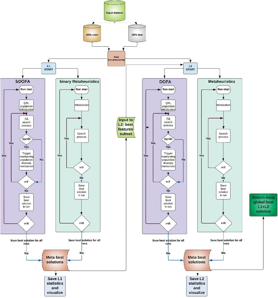
Figure 1 Visual representation of the devised two-level framework.
Metaheuristics are encoded by using a flat encoding scheme. The length of the solution depends on framework level. In L1 agents are represented as a vector with length , where represents the total number of features.
For L2, one individual represents a set of six XGBoost hyper-parameters that are tuned (). The list with respective boundaries is shown in Table 1.
Table 1 Optimized XGBoost hyper-parameters
| Parameter | Boundaries | Type |
| () | continuous | |
| continuous | ||
| continuous | ||
| continuous | ||
| integer | ||
| continuous |
The search space encompasses binary, discrete, and continuous variables making this problem a mixed optimization task. A combination of the binary (bDOFA) and standard continuous DOFA is utilized. The L1 framework uses bDOFA, while L2 employs standard DOFA. Following extensive testing, it has been observed that the sigmoid obtained the best results, therefore it is utilized for this research. All discrete parameters have been rounded up to the closest whole value. The equation used for the search function has not been adapted to work with a discrete space.
The objective function that is subjected to the minimization process in the L1 accounts for classification error rate () and the number of features (), given as:
| (10) |
where and are used to determine relative importance of to , where . The employed objective function is commonly used in feature selection challenges [1].
The L2 part of the framework uses as the objective function.
3 Experimental Setup and Results
3.1 Datasets
This work makes use of three publicly available datasets to evaluate the proposed framework. The first two datasts come from the Mendeley Phishing Websites Dataset [20] available at https://data.mendeley.com/datasets/72ptz43s9v/, comprised of a full and small variant. With 111 features it is computationally expensive. Therefore, 20% of the smaller and full variant are used. The features list remains the same, but the number of instances is reduced to 11728 and 17729 entries in the small and full versions respectfully, and the same ratio of legitimate to phishing website examples is maintained. The second dataset is the UCI Phishing Websites Data Set provided by the University of California, Irvine (UCI) in their Machine Learning Repository and can be acquired from https://archive.ics.uci.edu/ml/datasets/phishing+websites. It consists of 6157 phishing URLs, and 4898 legitimate ones.
The small version of the Mendeley dataset is a relatively balanced dataset. While a second full Mendeley dataset is without about of the data representing phishing instances. The UCI dataset is also imbalanced as of the data represents legitimate instances. The distributions of legitimate to phishing data in all three dataset can be seen in Figure 2.

Figure 2 Phishing website datasets class distribution.
3.2 Experimental Setup
The behavior of the proposed DOFA algorithm has been verified on feature selection and XGBoost tuning problems using the described dataset. A comparative assessment has been carried out with other cutting-edge metaheuristics including: the original FA [21], BA [23]), ABC [11], HHO [9], SCA [14] and SNS [18]. All competitor algorithms were developed independently by the authors as part of this research, with the values of control parameters as proposed in their corresponding publications.
For the feature selection simulations (level 1), all metaheuristics were given the FS prefix, while the XGBoost prefix was added for XGBoost optimizing experiments (level 2). In all simulations, all metaheuristics were employed with the population of eight individuals (), with maximum 10 iterations () in one run, while the total number of runs was set to 30. However, since the FA in average case utilizes in each iteration, to generate objective comparative analysis, FA and DOFA were tested with only four individuals in the population. The third experiment unidentified identical settings, while using the Cohen’s kappa coefficient as an objective function and formulated as a maximization problem.
Additionally, for the L1 part of the framework, the k-nearest neighbor (KNN) with is chosen as the classifier with its default parameters from scikit-learn library. Values for and for the objective function (Equation (10)) were set to 0.95 and 0.05, respectively.
3.3 Results and Comparative Analysis
To show the introduced performance improvements, this paper presents a comparative analysis of the new method to other state-of-the-art algorithms tasked with the same task. The simulations were conducted in three sessions, described in the following.
3.3.1 Experiment I – Level 1 and level 2 of the framework
The best feature set determined within level 1 that is performing the feature selection, is further given as the input to level 2 that drives the XGBoost optimization. Table 2 shows the overall metrics for the feature selection problem on the level one of the proposed framework. Clearly, the suggested FS-DOFA achieved superior level of the performances on both small and full datasets in terms of best, worst, mean and median metrics, outperforming the FS-FA approach.
Table 2 Overall metrics for L1 results (feature selection)
| Method | FS-DOFA | FS-FA | FS-BA | FS-ABC | FS-HHO | FS-SCA | FS-SNS |
| small dataset | |||||||
| Best | 0.097246 | 0.101923 | 0.105527 | 0.105036 | 0.120615 | 0.101022 | 0.102642 |
| Worst | 0.103275 | 0.108362 | 0.135133 | 0.117148 | 0.127990 | 0.111064 | 0.113990 |
| Mean | 0.100060 | 0.105109 | 0.115597 | 0.112723 | 0.123717 | 0.106110 | 0.106876 |
| Median | 0.099860 | 0.105076 | 0.110864 | 0.114354 | 0.123131 | 0.106178 | 0.105436 |
| Std | 0.002262 | 0.002970 | 0.011497 | 0.004873 | 0.002895 | 0.003643 | 0.004270 |
| Var | 0.000005 | 0.000009 | 0.000132 | 0.000024 | 0.000008 | 0.000013 | 0.000018 |
| Best error | 0.089088 | 0.095908 | 0.095908 | 0.092072 | 0.098039 | 0.095908 | 0.097613 |
| Best no. feat. | 28 | 24 | 32 | 39 | 61 | 22 | 22 |
| full dataset | |||||||
| Best | 0.068387 | 0.072892 | 0.077811 | 0.081000 | 0.082754 | 0.073745 | 0.074803 |
| Worst | 0.071785 | 0.081453 | 0.078650 | 0.089317 | 0.095137 | 0.074499 | 0.087966 |
| Mean | 0.069580 | 0.077523 | 0.078210 | 0.084035 | 0.088571 | 0.073991 | 0.080962 |
| Median | 0.069075 | 0.077873 | 0.078190 | 0.082911 | 0.088197 | 0.073860 | 0.080539 |
| Std | 0.001304 | 0.003548 | 0.000315 | 0.003151 | 0.004394 | 0.000301 | 0.004681 |
| Var | 0.000002 | 0.000013 | 0.000000 | 0.000010 | 0.000019 | 0.000000 | 0.000022 |
| Best error | 0.063452 | 0.063452 | 0.067682 | 0.063452 | 0.069092 | 0.069092 | 0.061196 |
| Best no. feat. | 18 | 28 | 30 | 46 | 38 | 18 | 37 |
Table 3 shows the overall metrics for the XGBoost optimization task (level two of the observed framework). On the small dataset, the suggested XGBoost-DOFA obtained the best result, while XGBoost-FA achieved the first place in terms of worst, mean and median values. The best set of XGBoost parameters was obtained by XGBoost-DOFA, with the following values: . When dealing with the full dataset, XGBoost-FA obtained the best result, while the proposed XGBoost-DOFA was superior in terms of worst, mean and median values. The best set of the parameters was obtained by XGBoost-FA, with values , while the proposed XGBoost-DOFA determined the following parameter values: .
Table 3 Overall metrics for L1 + L2 results
| Method | XGBoost-DOFA | XGBoost-FA | XGBoost-BA | XGBoost-ABC | XGBoost-HHO | XGBoost-SCA | XGBoost-SNS |
| small dataset | |||||||
| Best | 0.066496 | 0.066922 | 0.067349 | 0.068627 | 0.069480 | 0.068627 | 0.067349 |
| Worst | 0.070759 | 0.070332 | 0.072890 | 0.075021 | 0.072464 | 0.072890 | 0.073316 |
| Mean | 0.069480 | 0.068841 | 0.069835 | 0.070759 | 0.070972 | 0.070404 | 0.070332 |
| Median | 0.070119 | 0.069054 | 0.069906 | 0.070332 | 0.070972 | 0.070119 | 0.070546 |
| Std | 0.001435 | 0.001094 | 0.001799 | 0.002029 | 0.001224 | 0.001505 | 0.001938 |
| Var | 0.000002 | 0.000001 | 0.000003 | 0.000004 | 0.000001 | 0.000002 | 0.000004 |
| Best no. feat. | 28 | 28 | 28 | 28 | 28 | 28 | 28 |
| full dataset | |||||||
| Best | 0.044557 | 0.045403 | 0.046249 | 0.045403 | 0.045403 | 0.044557 | 0.044839 |
| Worst | 0.047941 | 0.049069 | 0.050479 | 0.049915 | 0.051607 | 0.049069 | 0.049069 |
| Mean | 0.045544 | 0.046860 | 0.048176 | 0.046907 | 0.047706 | 0.046625 | 0.046249 |
| Median | 0.045262 | 0.046672 | 0.047659 | 0.045826 | 0.047377 | 0.046813 | 0.045826 |
| Std | 0.001113 | 0.001121 | 0.001640 | 0.001854 | 0.002305 | 0.001426 | 0.001382 |
| Var | 0.000001 | 0.000001 | 0.000003 | 0.000003 | 0.000005 | 0.000002 | 0.000002 |
| Best no. feat. | 18 | 18 | 18 | 18 | 18 | 18 | 18 |
Table 4 shows the detailed metrics on the small dataset, considering the best solutions after the execution of the entire framework (both levels, L1 + L2). In the case of a small dataset, the proposed XGBoost-DOFA method achieved the best accuracy of 94.46%. Table 5 depicts detailed metrics over the full dataset. In this scenario, the proposed XGBoost-DOFA obtained the accuracy of 94.54%, and shared the first place with XGBoost-SCA
Table 4 Detailed metrics for the best solutions with feature selection (L1+L2) on the small dataset
| XGBoost-DOFA | XGBoost-FA | XGBoost-BA | XGBoost-ABC | XGBoost-HHO | XGBoost-SCA | XGBoost-SNS | |
| Accuracy (%) | 93.3504 | 93.3078 | 93.2651 | 93.1373 | 93.0520 | 93.1373 | 93.2651 |
| Precision 0 | 0.930357 | 0.929527 | 0.931777 | 0.928508 | 0.925333 | 0.925466 | 0.931777 |
| Precision 1 | 0.936378 | 0.936327 | 0.933442 | 0.933985 | 0.935299 | 0.936833 | 0.933442 |
| M.Avg. Precision | 0.933504 | 0.933080 | 0.932647 | 0.931370 | 0.930541 | 0.931406 | 0.932647 |
| Recall 0 | 0.930357 | 0.930357 | 0.926786 | 0.927679 | 0.929464 | 0.931250 | 0.926786 |
| Recall 1 | 0.936378 | 0.935563 | 0.938010 | 0.934747 | 0.931485 | 0.931485 | 0.938010 |
| M.Avg. Recall | 0.933504 | 0.933078 | 0.932651 | 0.931373 | 0.930520 | 0.931373 | 0.932651 |
| F1 score 0 | 0.930357 | 0.929942 | 0.929275 | 0.928093 | 0.927394 | 0.928349 | 0.929275 |
| F1 score 1 | 0.936378 | 0.935945 | 0.935720 | 0.934366 | 0.933388 | 0.934151 | 0.935720 |
| M.Avg. F1 score | 0.933504 | 0.933079 | 0.932643 | 0.931371 | 0.930526 | 0.931381 | 0.932643 |
Table 5 Detailed metrics for the best solutions with feature selection (L1+L2) on the full dataset
| XGBoost-DOFA | XGBoost-FA | XGBoost-BA | XGBoost-ABC | XGBoost-HHO | XGBoost-SCA | XGBoost-SNS | |
| Accuracy (%) | 95.5443 | 95.4597 | 95.3751 | 95.4597 | 95.4597 | 95.5443 | 95.5161 |
| Precision 0 | 0.967561 | 0.969961 | 0.967071 | 0.969961 | 0.969961 | 0.970819 | 0.971628 |
| Precision 1 | 0.932739 | 0.926341 | 0.928918 | 0.926341 | 0.926341 | 0.927200 | 0.925100 |
| M.Avg. Precision | 0.955521 | 0.954880 | 0.953880 | 0.954880 | 0.954880 | 0.955738 | 0.955541 |
| Recall 0 | 0.964224 | 0.960345 | 0.962069 | 0.960345 | 0.960345 | 0.960776 | 0.959483 |
| Recall 1 | 0.938825 | 0.943719 | 0.938010 | 0.943719 | 0.943719 | 0.945351 | 0.946982 |
| M.Avg. Recall | 0.955443 | 0.954597 | 0.953751 | 0.954597 | 0.954597 | 0.955443 | 0.955161 |
| F1 Score 0 | 0.965889 | 0.965129 | 0.964564 | 0.965129 | 0.965129 | 0.965771 | 0.965517 |
| F1 Score 1 | 0.935772 | 0.934949 | 0.933442 | 0.934949 | 0.934949 | 0.936187 | 0.935913 |
| M.Avg. F1 Score | 0.955477 | 0.954695 | 0.953803 | 0.954695 | 0.954695 | 0.955543 | 0.955282 |
Convergence graphs of the objective function (L1), error (L2), and error (both L1 and L2) of all algorithms over both utilized datasets, are depicted in Figure 3. Box plots showing the dispersing of the objective function (L1), error (L2), and error (both L1 and L2), are presented in Figure 4.
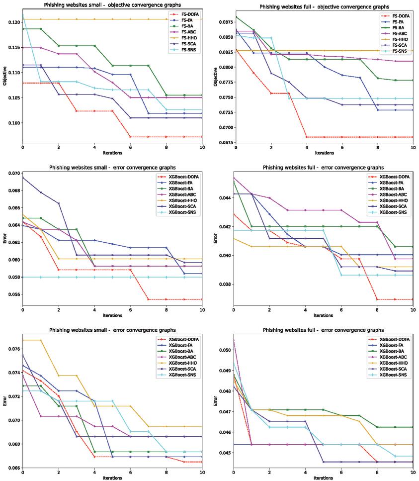
Figure 3 Convergence graphs of the objective function for L1 framework (first row), error for L2 framework (second row), and error for L1+L2 (third row), for all algorithms and both Manderley datasets.
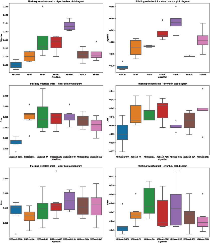
Figure 4 Box plots of the objective function for L1 (first row), error for L2 (second row) and error for L1 + L2 (third row), for all algorithms and both Manderley datasets.
PR curves of the outcomes of the L1 + L2 framework (output of level 2), for individual metaheuristics and both utilized datasets are shown in Figure 5. The ROC AUC micro-macro curves for the L1 + L2 framework are given in Figure 6.
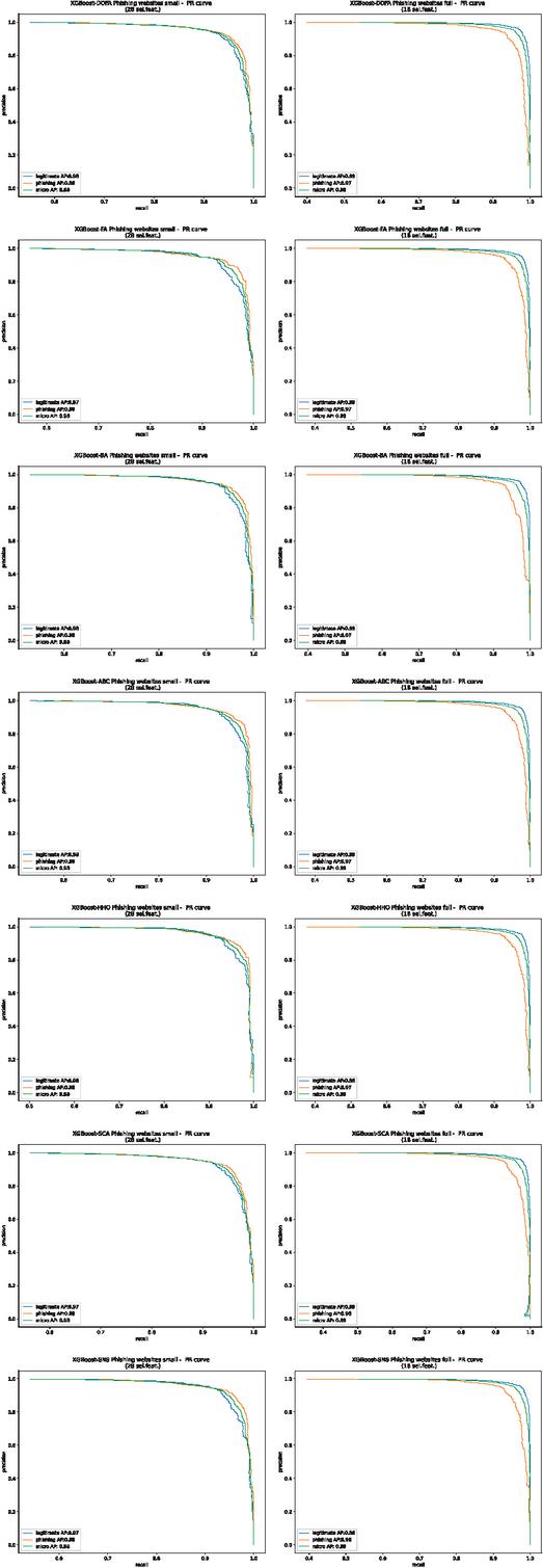
Figure 5 PR curves for L2 output (L1 + L2) for all algorithms and both Manderley datasets.
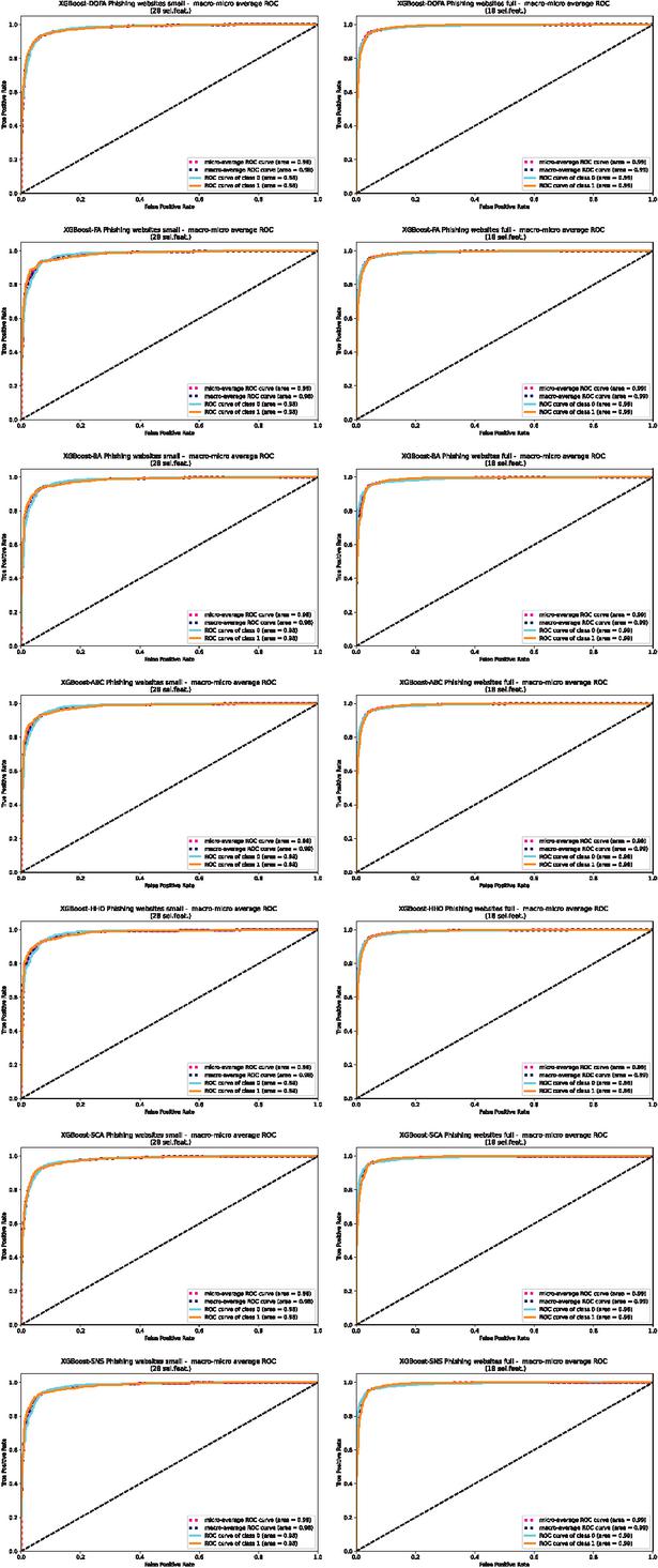
Figure 6 ROC AUC micro-macro curves for L2 output (L1 + L2), for all algorithms and both both Manderley datasets.
3.3.2 Experiment II – Level 2 of the framework
The second session of simulations focused on testing all algorithms for the XGBoost optimization problem, without feature selection. These experiments used only level 2 of the framework, and overall metrics are given in Table 6. Here, it is obvious that the proposed XGBoost-DOFA achieved superior results on both Manderley datasets.The best obtained set of XGBoost parameters on small dataset was determined by XGBoost-DOFA, and the values were . Concerning the full dataset, the best obtained set of XGBoost parameters was also determined by XGBoost-DOFA, with values .
When comparing, Table 3 gives the results of the XGBoost optimization with feature selection employed, and Table 6 exhibits the results of XGBoost tuning without feature selection (all features employed), the results are better in case feature selection was not utilized. This is expected, as the error rate is smaller if all features were used, but at the cost of higher computational complexity.
Table 6 Overall metrics for L2 results (no feature selection)
| Method | XGBoost-DOFA | XGBoost-FA | XGBoost-BA | XGBoost-ABC | XGBoost-HHO | XGBoost-SCA | XGBoost-SNS |
| small dataset | |||||||
| Best | 0.055413 | 0.058397 | 0.059250 | 0.059250 | 0.060102 | 0.059676 | 0.057971 |
| Worst | 0.058397 | 0.064365 | 0.067349 | 0.062660 | 0.064365 | 0.063086 | 0.062234 |
| Mean | 0.057190 | 0.061949 | 0.062305 | 0.061523 | 0.062020 | 0.061381 | 0.060315 |
| Median | 0.057545 | 0.062447 | 0.061594 | 0.062020 | 0.061807 | 0.061594 | 0.060529 |
| Std | 0.000934 | 0.001820 | 0.002864 | 0.001294 | 0.001320 | 0.001180 | 0.001471 |
| Var | 0.000001 | 0.000003 | 0.000008 | 0.000002 | 0.000002 | 0.000001 | 0.000002 |
| Best no. feat. | 111 | 111 | 111 | 111 | 111 | 111 | 111 |
| full dataset | |||||||
| Best | 0.036943 | 0.040045 | 0.040609 | 0.039763 | 0.039199 | 0.038917 | 0.038635 |
| Worst | 0.041173 | 0.043429 | 0.043429 | 0.043147 | 0.040609 | 0.041737 | 0.044275 |
| Mean | 0.039086 | 0.041342 | 0.041455 | 0.041737 | 0.039876 | 0.040496 | 0.041737 |
| Median | 0.038917 | 0.040609 | 0.040891 | 0.042301 | 0.039763 | 0.040609 | 0.042019 |
| Std | 0.001445 | 0.001306 | 0.001070 | 0.001236 | 0.000458 | 0.001049 | 0.001801 |
| Var | 0.000002 | 0.000002 | 0.000001 | 0.000002 | 0.000000 | 0.000001 | 0.000003 |
| Best no. feat. | 111 | 111 | 111 | 111 | 111 | 111 | 111 |
Tables 7 and 8 show the detailed metrics on the small and full datasets, for the best solutions without feature selection. The proposed XGBoost-DOFA has established superior performance in both scenarios, with the best accuracy of 93.35% on the small, and 96.31% on the full dataset.
Table 7 Detailed metrics for the best solutions without feature selection (L2) on the small dataset
| XGBoost-DOFA | XGBoost-FA | XGBoost-BA | XGBoost-ABC | XGBoost-HHO | XGBoost-SCA | XGBoost-SNS | |
| Accuracy (%) | 93.3504 | 93.3078 | 93.2651 | 93.1373 | 93.0520 | 93.1373 | 93.2651 |
| Precision 0 | 0.930357 | 0.929527 | 0.931777 | 0.928508 | 0.925333 | 0.925466 | 0.931777 |
| Precision 1 | 0.936378 | 0.936327 | 0.933442 | 0.933985 | 0.935299 | 0.936833 | 0.933442 |
| M.Avg. Precision | 0.933504 | 0.933080 | 0.932647 | 0.931370 | 0.930541 | 0.931406 | 0.932647 |
| Recall 0 | 0.930357 | 0.930357 | 0.926786 | 0.927679 | 0.929464 | 0.931250 | 0.926786 |
| Recall 1 | 0.936378 | 0.935563 | 0.93801 | 0.934747 | 0.931485 | 0.931485 | 0.938010 |
| M.Avg. Recall | 0.933504 | 0.933078 | 0.932651 | 0.931373 | 0.930520 | 0.931373 | 0.932651 |
| F1 Score 0 | 0.930357 | 0.929942 | 0.929275 | 0.928093 | 0.927394 | 0.928349 | 0.929275 |
| F1 Score 1 | 0.936378 | 0.935945 | 0.935720 | 0.934366 | 0.933388 | 0.934151 | 0.935720 |
| M.Avg. F1 Score | 0.933504 | 0.933079 | 0.932643 | 0.931371 | 0.930526 | 0.931381 | 0.932643 |
Table 8 Detailed metrics for the best solutions without feature selection (L2) on the full dataset
| XGBoost-DOFA | XGBoost-FA | XGBoost-BA | XGBoost-ABC | XGBoost-HHO | XGBoost-SCA | XGBoost-SNS | |
| Accuracy (%) | 96.3057 | 95.9955 | 95.9391 | 96.0237 | 96.0801 | 96.1083 | 96.1365 |
| Precision 0 | 0.970348 | 0.969802 | 0.968966 | 0.970626 | 0.970246 | 0.968643 | 0.970677 |
| Precision 1 | 0.949139 | 0.941368 | 0.941272 | 0.940699 | 0.942950 | 0.946634 | 0.943765 |
| M.Avg. Precision | 0.963015 | 0.959971 | 0.959391 | 0.960279 | 0.960809 | 0.961033 | 0.961373 |
| Recall 0 | 0.973276 | 0.968966 | 0.968966 | 0.968534 | 0.969828 | 0.971983 | 0.970259 |
| Recall 1 | 0.943719 | 0.942904 | 0.941272 | 0.944535 | 0.943719 | 0.940457 | 0.944535 |
| M.Avg. Recall | 0.963057 | 0.959955 | 0.959391 | 0.960237 | 0.960801 | 0.961083 | 0.961365 |
| F1 Score 0 | 0.971810 | 0.969383 | 0.968966 | 0.969579 | 0.970037 | 0.970310 | 0.970468 |
| F1 Score 1 | 0.946421 | 0.942135 | 0.941272 | 0.942613 | 0.943335 | 0.943535 | 0.944150 |
| M.Avg. F1 Score | 0.963032 | 0.959963 | 0.959391 | 0.960256 | 0.960805 | 0.961053 | 0.961369 |
One vs. One (OvO) ROC curves for full dataset, and One vs. Rest (OvR) ROC curves for the small dataset are presented in Figures 7 and 8 respectively. The relation of each class to other classes, together with their distribution, can be seen on histograms that are also provided in Figure 8.
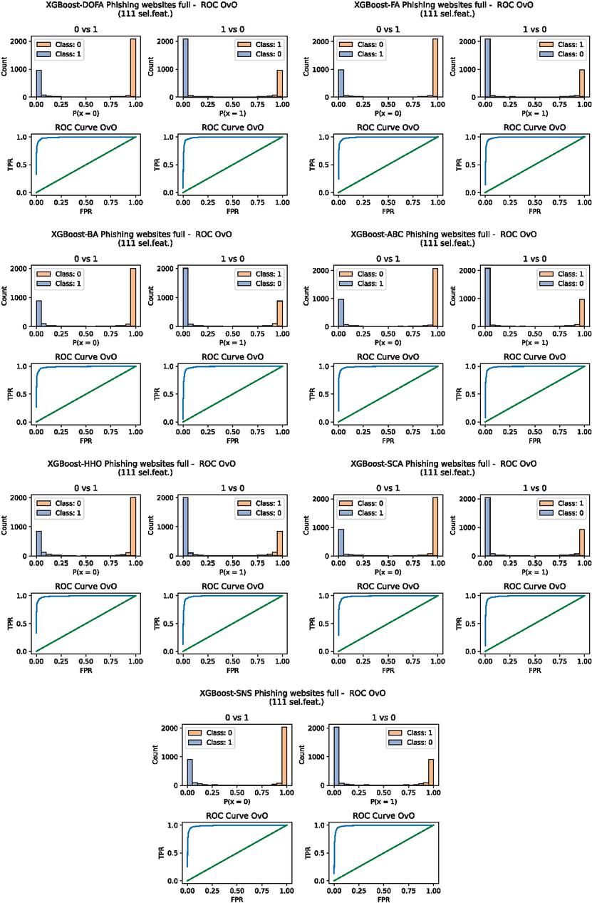
Figure 7 One vs. One (OvO) ROC curves for the best solutions (smallest error) of L2 without feature selection on the full dataset.
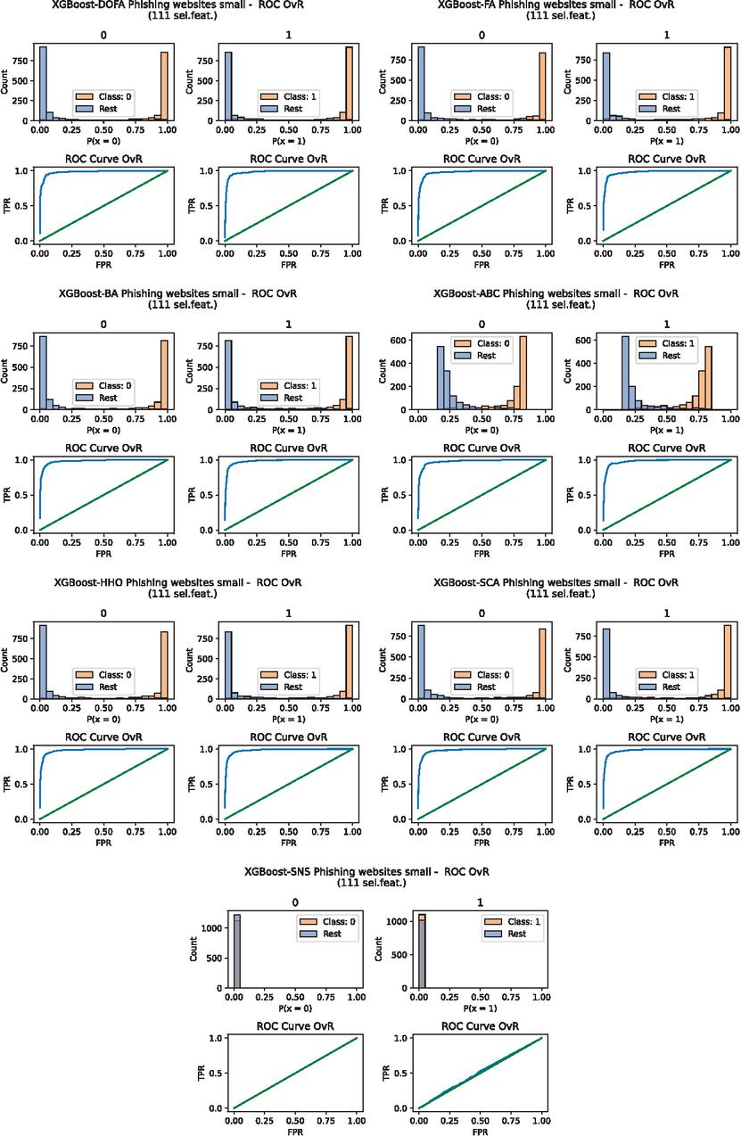
Figure 8 One vs. Rest (OvR) ROC curves for the best solutions (smallest error) of L2 without feature selection for the small dataset.
3.3.3 Experiment III – Level 2 of the framework on the UCI dataset
The third experimental simulations on evaluation several metaheuristics performance for tuning XGboost, without feature selection. These experiments relied only on level 2 of the framework. The objective function used to guide the optimization is Cohen’s kappa [19], as it demonstrated better evaluations when assessing performance on unbalanced data. The overall metrics are shown in Table 9, while Table 10 shows detailed metrics for each tested metaheuristic on the UCI dataset.
Finally to better demonstrate the improvements made by the implemented modification in the novel proposed algorithm, error and objective function convergence graphs are shown in Figure 9, followed by violin plots for both. The results shown suggest that the improvements made show an increased convergence rate compared to the original metaheuristic. Additionally, more consistent grouping is demonstrated for both objective function and error rates over 10 independent runs indicating more reliable performance.
Further improvements demonstrated on the novel metaheuristics are presented in Figure 10, where diversity swarm plots for the final iteration of each run are presented. As indicated by the results a much higher population diversity is achieved by the introduced metaheuristic.
Table 9 Overall metrics for L2 tests with the UCI dataset
| Method | XGBoost-DOFA | XGBoost-FA | XGBoost-BA | XGBoost-ABC | XGBoost-HHO | XGBoost-SCA | XGBoost-SNS |
| Best | 0.951315 | 0.950423 | 0.950485 | 0.946761 | 0.950485 | 0.947685 | 0.947728 |
| Worst | 0.943114 | 0.930370 | 0.930370 | 0.930370 | 0.930370 | 0.930370 | 0.930370 |
| Mean | 0.947144 | 0.942659 | 0.945043 | 0.940205 | 0.944142 | 0.942113 | 0.943580 |
| Median | 0.947701 | 0.946761 | 0.947234 | 0.946761 | 0.946761 | 0.946761 | 0.946761 |
| Std | 0.002650 | 0.007759 | 0.007290 | 0.008030 | 0.006979 | 0.007325 | 0.006611 |
| Var | 0.000007 | 0.000060 | 0.000053 | 0.000064 | 0.000049 | 0.000054 | 0.000044 |
| Best error | 0.023971 | 0.024423 | 0.024423 | 0.026232 | 0.024423 | 0.025780 | 0.025780 |
| Best no. feat. | 30 | 30 | 30 | 30 | 30 | 30 | 30 |
Table 10 Detail metrics for L2 tests with the UCI dataset
| XGBoost-DOFA | XGBoost-FA | XGBoost-BA | XGBoost-ABC | XGBoost-HHO | XGBoost-SCA | XGBoost-SNS | |
| Accuracy (%) | 97.6029 | 97.5577 | 97.5577 | 97.3768 | 97.5577 | 97.4220 | 97.4220 |
| Precision 0 | 0.984326 | 0.981289 | 0.975359 | 0.978216 | 0.975359 | 0.978238 | 0.974306 |
| Precision 1 | 0.969697 | 0.971177 | 0.975748 | 0.970329 | 0.975748 | 0.971108 | 0.974152 |
| M.Avg. Precision | 0.976181 | 0.975659 | 0.975576 | 0.973825 | 0.975576 | 0.974268 | 0.974220 |
| Recall 0 | 0.961224 | 0.963265 | 0.969388 | 0.962245 | 0.969388 | 0.963265 | 0.967347 |
| Recall 1 | 0.987815 | 0.985378 | 0.980504 | 0.982941 | 0.980504 | 0.982941 | 0.979691 |
| M.Avg. Recall | 0.976029 | 0.975577 | 0.975577 | 0.973768 | 0.975577 | 0.974220 | 0.974220 |
| F1 score 0 | 0.972638 | 0.972194 | 0.972364 | 0.970165 | 0.972364 | 0.970694 | 0.970814 |
| F1 score 1 | 0.978672 | 0.978226 | 0.978120 | 0.976594 | 0.978120 | 0.976988 | 0.976914 |
| M.Avg. F1 score | 0.975998 | 0.975552 | 0.975569 | 0.973744 | 0.975569 | 0.974198 | 0.974210 |
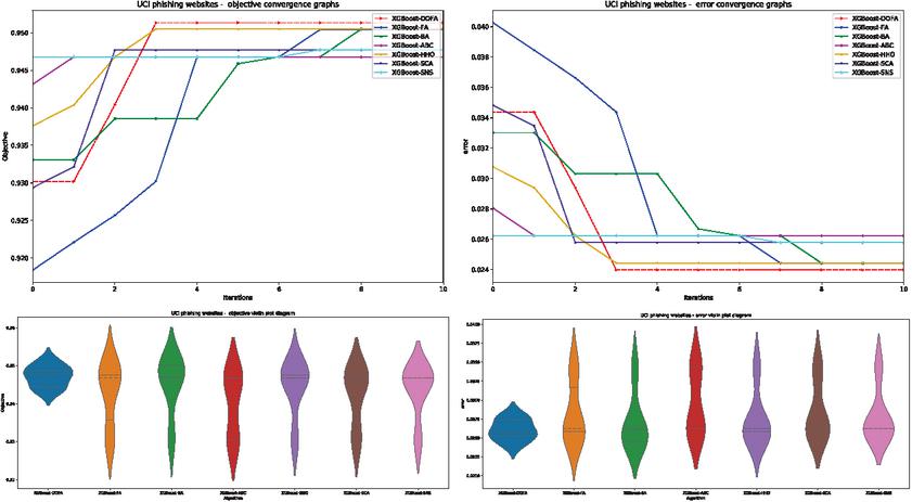
Figure 9 Objective function and error convergence grate graphs on the UCI dataset (above) objective function and error violin plots (below).
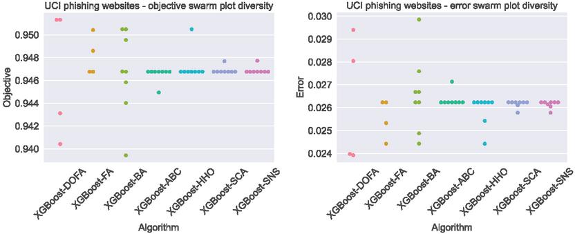
Figure 10 Objective function and error swarm plots of individuals in the final iteration of the best run for UCI dataset.
3.4 Validation of Achieved Results and SHAP Model Interpretation
Judging algorithms based on experimental results is not always sufficient to define improvements. The seven methods used in this research have all been put to statistical comparison to determine the improvements made.
Following recommendations for previous works tackling similar subjects [4, 6], the sample results of each method are taken based on the average values of measured objectives. This research uses objective function classification error rates that have been used for testing, averaged following 50 independent runs. The decision to do so has been made following several conducted Shapiro–Wilk [16] tests for single-problem analysis [6].
The justification for the use of parametric test conditions is so that the independence, normality, and homoscedasticity of the variances of the data has been assessed [12]. Each execution was conducted separately. Conditions are evaluated with the Shapiro–Wilk test [16], with results given in Table 11.
Table 11 Shapiro multiple statistical test results
| DOFA | FA | BA | ABC | HHO | SCA | SNS |
| 0.0113 | 0.0132 | 0.01346 | 0.0234 | 0.0338 | 0.0113 | 0.0305 |
To evaluate homoscedasticity based on mean values, Levene’s test [8] is used, with the resulting -value being 0.64, meaning that the homoscedasticity criteria are met.
It is important to note that the Shapiro–Wilk test resulting in -values for all methods is less than the criteria as shown in Table 11. Therefore, parametric test criteria is not satisfied. For non-parametric testing, the proposed DOFA has been established as the control method.
To determine how significant the performance improvement of the proposed algorithm is when compared to other methods, the Friedman test [7] and two-way variance analysis by ranks were constructed, as per recommendations in [4]. The results of the Friedman test are shown in Table 12.
Table 12 Friedman statistical test results
| Functions | DOFA | FA | BA | ABC | HHO | SCA | SNS |
| l1 small | 1 | 5 | 6 | 4 | 7 | 2 | 3 |
| l1+l2 small | 1 | 3 | 2 | 6 | 7 | 5 | 4 |
| l2 small | 1 | 5 | 7 | 4 | 6 | 3 | 2 |
| l1 full | 1 | 3 | 4 | 6 | 7 | 2 | 5 |
| l1+l2 full | 1 | 4 | 7 | 5 | 6 | 3 | 2 |
| l2 full | 1 | 4 | 5 | 6.5 | 2 | 3 | 6.5 |
| l2 UCI | 1 | 4 | 3 | 7 | 2 | 6 | 5 |
| Average ranking | 1 | 4 | 4.8571 | 5.50 | 5.2857 | 3.4285 | 3.9256 |
| Rank | 1 | 4 | 5 | 7 | 6 | 2 | 3 |
Based on the statistical indications of the results from Table 12 the proposed DOFA approach presents improved performance compared to other algorithms, with the average attaining the rank of 1. The Friedman statistics criteria are fulfilled, rejecting the null hypothesis (), signifying that the novel DOFA algorithm attained notably improved performance as opposed to other competitors.
As [17] suggests, the Iman and Davenport’s is used with a result , notably higher than the threshold value of the -distribution (), and the -value is . Accordingly, this test also rejects .
Due to both tests rejecting the null hypothesis, the non-parametric post-hoc Holm’s step-down procedure was applied. The results are shown in Table 13. The results are sorted with respect to values, evaluated to , where and represent the degrees of freedom ( for this research). Algorithms are sorted in ascending order according to the value. Values used for are 0.05 and 0.1 in the conducted experiment. The results shown in Table 13 clearly indicate the proposed algorithm drastically outperforms other contemporary algorithms at both significance levels.
Table 13 Holm’s step-down procedure statistical test results
| Comparison | p_values | Ranking | alpha = 0.05 | alpha = 0.1 | H1 | H2 |
| DOFA vs HHO | 5.32E-05 | 0 | 0.0083 | 0.0167 | 1 | 1 |
| DOFA vs ABC | 3.28E-04 | 1 | 0.0100 | 0.0200 | 1 | 1 |
| DOFA vs BA | 4.18E-04 | 2 | 0.0125 | 0.0250 | 1 | 1 |
| DOFA vs FA | 8.08E-03 | 3 | 0.0167 | 0.0333 | 1 | 1 |
| DOFA vs SNS | 1.37E-02 | 4 | 0.0250 | 0.0500 | 1 | 1 |
| DOFA vs SCA | 5.44E-02 | 5 | 0.0500 | 0.1000 | 0 | 1 |
The best performing model from experiment 3 was additionally interpreted using via SHapley Additive exPlanations (SHAP) [13]. Feature impacts can be observed in Figure 11. Additionally, by observing Figure 12 feature impacts of all 30 features per class can be observed.

Figure 11 SHAP analysis summary plot for all features for UCI dataset.
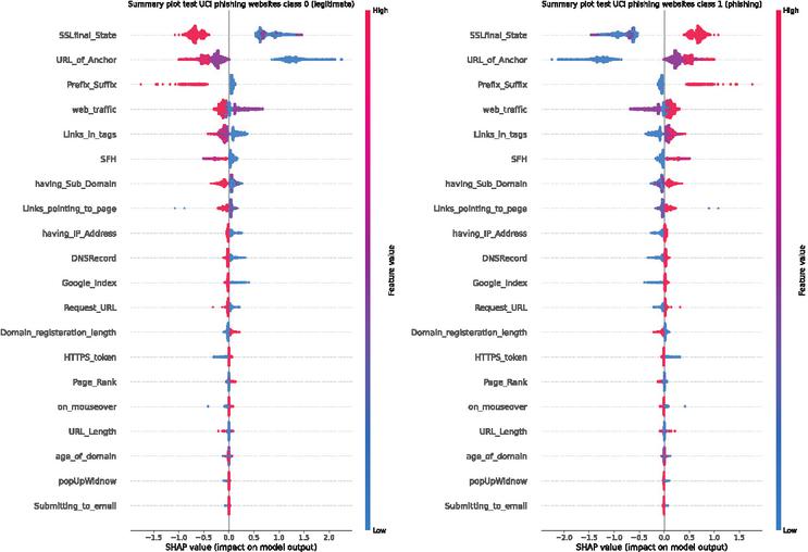
Figure 12 SHAP analysis plot per class for all features for UCI dataset.
As indicated by SHAP analysis SSL certificates play an important role when identifying phishing websites. Anchor URLs play a close second, followed by prefixes and suffix data as well as traffic data.
4 Conclusion
This research proposed a novel variant of the FA algorithm, developed to overcome known shortcomings of the basic FA implementation. The algorithm was named diversity oriented firefly algorithm – DOFA, and employed in a framework to tune the XGBoost machine learning model. The proposed DOFA was used for both a feature selection task (L1 of the framework) and hyper-parameter tuning (L2 of the framework). This model was evaluated on a three known phishing benchmark dataset.
The results obtained by the proposed XGBoost-DOFA model were evaluated and compared with six other cutting-edge metaheuristics, which were employed in the same experimental setup. The obtained experimental results, as well as the conducted statistical tests, clearly indicate the superior performance of the proposed model and demonstrate the effectiveness of the proposed framework.
The future work in this area will include further testing of other machine learning models in the two layer framework to additionally explore the potential of the framework. In addition, the proposed model will be evaluated on other datasets, in order to establish even more confidence in the performance, before employing it in real-world systems.
References
[1] Benyamin Abdollahzadeh and Farhad Soleimanian Gharehchopogh. A multi-objective optimization algorithm for feature selection problems. Engineering with Computers, pages 1–19, 2021.
[2] Nadheera AlHosni, Luka Jovanovic, Milos Antonijevic, Milos Bukumira, Miodrag Zivkovic, Ivana Strumberger, Joseph P Mani, and Nebojsa Bacanin. The xgboost model for network intrusion detection boosted by enhanced sine cosine algorithm. In International Conference on Image Processing and Capsule Networks, pages 213–228. Springer, 2022.
[3] Shi Cheng and Yuhui Shi. Diversity control in particle swarm optimization. In 2011 IEEE Symposium on Swarm Intelligence, pages 1–9. IEEE, 2011.
[4] Joaquín Derrac, Salvador García, Daniel Molina, and Francisco Herrera. A practical tutorial on the use of nonparametric statistical tests as a methodology for comparing evolutionary and swarm intelligence algorithms. Swarm and Evolutionary Computation, 1(1):3–18, 2011.
[5] Dheeru Dua and Casey Graff. UCI machine learning repository, 2017.
[6] Tome Eftimov, Peter Korošec, and B Koroušic Seljak. Disadvantages of statistical comparison of stochastic optimization algorithms. Proceedings of the Bioinspired Optimizaiton Methods and their Applications, BIOMA, pages 105–118, 2016.
[7] Milton Friedman. The use of ranks to avoid the assumption of normality implicit in the analysis of variance. Journal of the american statistical association, 32(200):675–701, 1937.
[8] Gene V Glass. Testing homogeneity of variances. American Educational Research Journal, 3(3):187–190, 1966.
[9] Ali Asghar Heidari, Seyedali Mirjalili, Hossam Faris, Ibrahim Aljarah, Majdi Mafarja, and Huiling Chen. Harris hawks optimization: Algorithm and applications. Future generation computer systems, 97:849–872, 2019.
[10] Dijana Jovanovic, Milos Antonijevic, Milos Stankovic, Miodrag Zivkovic, Marko Tanaskovic, and Nebojsa Bacanin. Tuning machine learning models using a group search firefly algorithm for credit card fraud detection. Mathematics, 10(13):2272, 2022.
[11] Dervis Karaboga. Artificial bee colony algorithm. scholarpedia, 5(3):6915, 2010.
[12] Antonio LaTorre, Daniel Molina, Eneko Osaba, Javier Poyatos, Javier Del Ser, and Francisco Herrera. A prescription of methodological guidelines for comparing bio-inspired optimization algorithms. Swarm and Evolutionary Computation, 67:100973, 2021.
[13] Scott M Lundberg and Su-In Lee. A unified approach to interpreting model predictions. In I. Guyon, U. V. Luxburg, S. Bengio, H. Wallach, R. Fergus, S. Vishwanathan, and R. Garnett, editors, Advances in Neural Information Processing Systems 30, pages 4765–4774. Curran Associates, Inc., 2017.
[14] Seyedali Mirjalili. Sca: a sine cosine algorithm for solving optimization problems. Knowledge-based systems, 96:120–133, 2016.
[15] S. Rahnamayan, H. R. Tizhoosh, and M. M. A. Salama. Quasi-oppositional differential evolution. In 2007 IEEE Congress on Evolutionary Computation, pages 2229–2236, 2007.
[16] Samuel S Shapiro and RS Francia. An approximate analysis of variance test for normality. Journal of the American statistical Association, 67(337):215–216, 1972.
[17] David J Sheskin. Handbook of parametric and nonparametric statistical procedures. Chapman and Hall/CRC, 2020.
[18] Siamak Talatahari, Hadi Bayzidi, and Meysam Saraee. Social network search for global optimization. IEEE Access, 9:92815–92863, 2021.
[19] Susana M Vieira, Uzay Kaymak, and João MC Sousa. Cohen’s kappa coefficient as a performance measure for feature selection. In International conference on fuzzy systems, pages 1–8. IEEE, 2010.
[20] G Vrbancic. Phishing websites dataset. Mendeley Data, 1, 2020.
[21] Xin-She Yang. Firefly algorithms for multimodal optimization. In International symposium on stochastic algorithms, pages 169–178. Springer, 2009.
[22] Xin-She Yang. Firefly algorithms for multimodal optimization. In Osamu Watanabe and Thomas Zeugmann, editors, Stochastic Algorithms: Foundations and Applications, pages 169–178, Berlin, Heidelberg, 2009. Springer Berlin Heidelberg.
[23] Xin-She Yang. Bat algorithm for multi-objective optimisation. International Journal of Bio-Inspired Computation, 3(5):267–274, 2011.
[24] Xin-She Yang and He Xingshi. Firefly algorithm: Recent advances and applications. International Journal of Swarm Intelligence, 1(1):36–50, 2013.
[25] Miodrag Zivkovic, Luka Jovanovic, Milica Ivanovic, Nebojsa Bacanin, Ivana Strumberger, and P Mani Joseph. Xgboost hyperparameters tuning by fitness-dependent optimizer for network intrusion detection. In Communication and Intelligent Systems, pages 947–962. Springer, 2022.
Biographies

Luka Jovanovic is a junior researcher at Singidunum University. He is presently pursuing a bachelors degree in software engineering. His current research interests include areas of hardware security, artificial intelligence, machine learning and metaheuristics optimization.

Dijana Jovanovic received B.Sc. and M.Sc. degrees from the Department of Informatics at the College of Academic Studies “Dositej” in 2018 and 2019, respectively. She received her Ph.D. degree from Faculty of Computer Science, Megatrend University of Belgrade, Serbia. She is currently working as a research assistant at the College of Academic Studies “Dositej”.

Milos Antonijevic has a Ph.D. in computer sciences (study program Advanced security systems) from Singidunum University and a Masters degree of Engineer of Organizational Sciences from Faculty of Organizational sciences, University of Belgrade. He currently works as an Assistant professor at Singidunum University, Belgrade, Serbia and as a certified ISO 27001 Auditor for various accreditation authorities.

Bosko Nikolic is a Full Professor at the University of Belgrade, School of Electrical Engineering, Department for Computer Science and Information Technology. He received his Ph.D. degree in electrical and computer engineering from the University of Belgrade, School of Electrical Engineering, Belgrade, Serbia. His current research interests include the areas of artificial intelligence, web programming, visual simulation, natural language processing (NLP) and engineering education.

Nebojsa Bacanin received his Ph.D. degree from Faculty of Mathematics, University of Belgrade in 2015. He started his university career in Serbia 16 years ago at Graduate School of Computer Science in Belgrade. He currently works as a full professor and as a vice-rector for scientific research at Singidunum University, Belgrade, Serbia. He has also been included in the prestigious Stanford University list of the best 2% world researchers for the years 2020 and 2021.

Miodrag Zivkovic received his Ph.D. degree from School of Electrical Engineering, University of Belgrade in 2014. He started his university career in Serbia in 2016 at Singidunum University in Belgrade. He currently works as an associate professor at Faculty of Informatics and Computing, Singidunum University, Belgrade, Serbia. His current research interests include the areas of artificial intelligence, swarm intelligence, and optimization metaheuristics.

Ivana Strumberger started her University career in 2013 as a teaching assistant at Faculty of Computer Science in Belgrade. She received her P.h.D. degree from Singidunum University in 2020 from the domain of Computer Science. She has published around 50 scientific papers in high quality journals and international conferences. She has also published 10 book chapters in the Springer Lecture Notes in Computer Science series. She is regular reviewer of many international state-of-the-art journals. She has been included in the prestigious Stanford University list of the best 2% world scientists for the year 2021.
Journal of Web Engineering, Vol. 22_3, 543–574.
doi: 10.13052/jwe1540-9589.2237
© 2023 River Publishers