How to Retrieve Music using Mood Tags in a Folksonomy
Chang Bae Moon1, Jong Yeol Lee2 and Byeong Man Kim2,*
1ICT-Convergence Research Center, Kumoh National Institute of Technology, Korea
2Computer and Software Engineering, Kumoh National Institute of Technology, Korea
E-mail: cb.moon@kumoh.ac.kr; soyeum@kumoh.ac.kr; bmkim@kumoh.ac.kr
*Corresponding Author
Received 18 March 2021; Accepted 27 July 2021; Publication 06 November 2021
Abstract
A folksonomy is a classification system in which volunteers collaboratively create and manage tags to annotate and categorize content. The folksonomy has several problems in retrieving music using tags, including problems related to synonyms, different tagging levels, and neologisms. To solve the problem posed by synonyms, we introduced a mood vector with 12 possible moods, each represented by a numeric value, as an internal tag. This allows moods in music pieces and mood tags to be represented internally by numeric values, which can be used to retrieve music pieces. To determine the mood vector of a music piece, 12 regressors predicting the possibility of each mood based on acoustic features were built using Support Vector Regression. To map a tag to its mood vector, the relationship between moods in a piece of music and mood tags was investigated based on tagging data retrieved from Last.fm, a website that allows users to search for and stream music. To evaluate retrieval performance, music pieces on Last.fm annotated with at least one mood tag were used as a test set. When calculating precision and recall, music pieces annotated with synonyms of a given query tag were treated as relevant. These experiments on a real-world data set illustrate the utility of the internal tagging of music. Our approach offers a practical solution to the problem caused by synonyms.
Keywords: Music mood, folksonomy, mood tag, Last.fm, mood vector, relationship between mood and tag.
1 Introduction
Music retrieval can currently be categorized into five general types: query-by-text, query-by-humming, query-by-part, query-by-example, and query-by-class. A query-by-text system searches music pieces by bibliographical information (e.g., author, music title, and genre) saved in the music information database, operating in the same way as a text-based information retrieval system. In query-by-humming, the user input of humming is the query, and the system searches for pieces with similar melodies. A query-by-part system can be used, for example, by users who liked music that was playing in a restaurant; in this type of query, users input a clip of the music as a query, but may not know the title or even the main melody. A query-by-example system finds similar music pieces to a specific piece provider by a user; such a system differs from the query-by-part system only in that the entire piece, as opposed to a clip, is given as input. Further, users can also supply the music title as a query instead of actual music in a query-by-example system, while actual music must be provided when searching via query-by-part. In a query-by-class search, pieces must be classified in advance by genre or mood, and are later searched using an existing taxonomy.
Among the five retrieval methods, query-by-humming, query-by-part, and query-by-example are not general, but are only usable in specific situations (i.e., when the user can provide the music itself, or at least its central melody); query-by-text and query-by-class are more general methods. However, both of these methods require the intervention of experts or operators who process and tag each piece of music. Each time a new piece of music is added to the database, someone must input bibliographical information or classify it based on an established taxonomy. As new music is constantly being released, such a method is problematic. One possible solution to staying abreast of new music is to use automatic tagging based on an established taxonomy. Such systems automatically supply bibliographical information, as well as codes classifying musical features, genre, etc. However, such a method requires a manager (e.g., librarian, operator) to manually classify items based on an established taxonomy. Expanding this taxonomy to accommodate new categories and codes may be difficult, as it requires an in-depth knowledge of the structure of the taxonomy. Further, although one specific meaning may be intended per designated category, tabs may, in fact, have multiple meanings, decreasing the utility of the classification system.
Folksonomies have recently appeared as an alternative type of taxonomy. A folksonomy is a classification system in which volunteers collaboratively create and manage tags to annotate and categorize content. The problems of expanding taxonomies and ensuring exclusive meanings for tags can be partially addressed by the use of folksonomies. However, folksonomies do tend to have problems relating to tags. The first problem is that different users may use different words to express identical meanings; for example, a soothing piece of music may be tagged by two different users as “placid” and “calm,” respectively. The second problem is one of tagging level; i.e., the same root word may be used with modifiers to express different degrees of meaning (e.g., “placid” as opposed to “very placid.”). The final problem is that users may choose labels that have multiple meanings; for example, music described as “edgy” could be interpreted as being “avant-garde,” “experimental,” or “intense.” It may also have a personal meaning for a specific volunteer or musical subculture, introducing the problem of neologisms, which are common in slang and youth culture. In this paper, our goal is to solve the problems associated with synonyms when retrieving music. To do this, the mood vector (12 values representing different moods according to Thayer’s two-dimensional mood model) is introduced as an internal tag. Using this method, moods of music pieces and mood tags are all represented internally by numeric values; pieces identified as having moods similar to the mood tags of a query can then be retrieved based on the similarity of their mood vectors, even if their tags do not exactly match the query.
In the present paper, the relationship between folksonomy mood tags are mapped, their mood vectors are defined, and their correlations are analysed. Further, we suggest a music retrieval method based on this mapping information and perform a range of experiments using a test set made up of Last.fm mood tags and their synonyms.
2 Related Studies
Existing emotion models include the Russell model [1] (Figure 1a), the Hevner Model [2] (Figure 1b), and the Thayer model [3] (Figure 1c). Since both the Russell and Hevner models use adjectives to describe emotions, ambiguity arises if adjectives have multiple meanings. For this reason, the Thayer’s two-dimensional model is used, in which each mood or emotion is expressed by two values, arousal and valence. Arousal refers to the strength of stimulation that listeners feel (i.e., weak or powerful) and valence refers to the intrinsic attractiveness (positive valence) or aversiveness (negative valence). Figure 1c [12, 18] shows the relationships among 12 adjectives of mood and emotion in Thayer’s two-dimensional model.
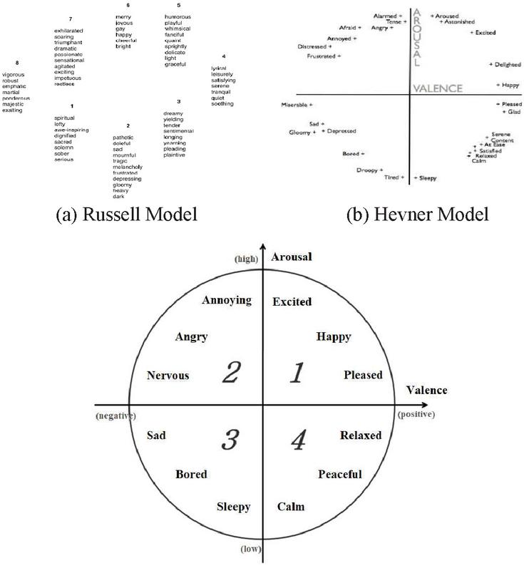
Figure 1 Music mood models.
Liu [4] has presented a music mood recognition system that uses a fuzzy classifier to categorize a waltz by Johann Strauss into five classes using the features including tempo, strength, pitch change, note density, and timbre. Katayose [5] has proposed a sentiment extraction system for pop music whereby sound data of monody are first converted into music code, from which melody, rhythm, harmony, and form are extracted. These two systems are useful in themselves, but they use Musical Instrument Digital Interface (MIDI; i.e., symbolic) expression, as it is difficult to extract useful features from sound data. However, much of the sound present in the real world cannot be expressed through symbols; no system exists that can correctly translate such sound data into symbolic expressions [22]. This limitation necessitates a system that can directly detect mood from sound data.
Feng et al. [6] have proposed a method of classifying moods into four groups—happiness, sadness, anger, and fear using tempo and articulation features. Li et al. [7] have proposed a method of detecting mood using timbre, texture, rhythm, and pitch features, using 13 adjective groups based on checklists by Hevner [8] and Farnsworth [9] as mood classes. Yang et al. [10] used a fuzzy-based method to solve the ambiguity of expression that can occur when only a single mood is allowed; they expressed musical mood as a mix of several moods, denoted as separate numerical values. However, Yang et al. noted that this method might fail to take into account subjective individual preferences, which would be necessary for personalized service [11, 12]. To solve this, rather than using a single mood class, they used AV (Arousal–Valence) values composed of two real number values between 1 and 1 on each axis of Thayer’s two-dimensional mood model. They used two regressors to model AV values collected from subjects and suggested a personalized detection method that characterizes users into “professional” or “non-professional” groups depending on their degree of musical understanding.
A number of studies have explored music folksonomy tags [15–17, 25]. In Laurier et al.’s and Kim et al.’s studies [16, 17, 25], music mood tags from the well-known folksonomy site Last.fm were treated as categories, upon which these authors constructed classification models. These classification models first determine the category of each piece of music, and then the folksonomy tag corresponding to the category is applied. In Steven et al.’s study [15], music was subdivided into sub-units and features were extracted. Then, these features were learned using a Support Vector Machine (SVM). When a new music piece is inputted, a mood tag is assigned based on the classification model.
3 Music Mood Retrieval Based on Folksonomy Tags
The object of the present paper is composed of three phases (Figure 2). The first phase is to create a prediction model for each mood; once the mood vector of the music piece is obtained, it is attached as an internal tag. The second phase is to define the mapping relationship between folksonomy tags on Last.fm and their mood vectors. The last phase is to retrieve music using mood vectors and tag-mood mapping information.
3.1 Creating Music Mood Vectors
Last.fm, a prominent online example of music folksonomy in action, boasts more than 1,000 music pieces that have at least one music mood tag. These pieces can be collected using API (Application Programming Interface). However, users provide mood tags in the form of words, not in the form of a mood vector. In order to accurately translate these tags and reflect users’ individual intended meanings for terms with multiple possible meanings, we would need to obtain individual mood vectors from all users. However, such an approach is impractical, and would be both time-consuming and prohibitively expensive. For this reason, models to predict the mood vector of a given music piece using existing music mood data [14] are built.
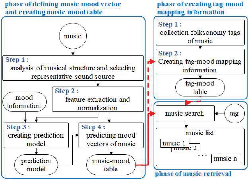
Figure 2 Overview of music retrieval system.
3.1.1 Analysis of musical structure
In prior studies, music pieces were separated into segments through musical structural analysis [13, 14, 18]. After obtaining these segments, each segment is separated into 12-second chunks according to the method developed by Kim et al. [23]. All segments of less than 12 seconds were discarded. Three music segments were chosen for each piece: one from the “Intro” section, one from the “Outro” section, and the one with the highest energy. The three selected music segments were then used to represent the entire music piece. For some music pieces, only two music segments were selected, as the music segment with the highest energy coincided with the Intro or Outro.
3.1.2 Feature extraction and normalization
In this paper, the 391 features are extracted using Lartillot’s MIR toolbox [19] (see Figure 3). However, when features are extracted using MIR toolbox, NaNs—values that cannot be expressed numerically—may occur. Features with at least one NaN were removed, as well as features whose value was the same for all segments; for this reason, the final number of features used in our experiments was 330. While the difference between minimum and maximum values exceeded 3,000 for some features, it was below 0.07 for others. The feature values may also be positive or negative. Thus, in our experiments, feature values were normalized between 1 and 1 by use of Equation (1), where is the ’th feature value of the ’th data in the class c and is its normalized value.
| (1) | |
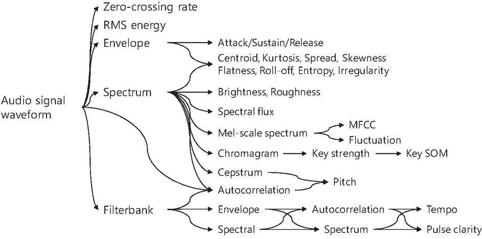
Figure 3 Overview of the features extraction in MIR Tollbox.
3.1.3 Building prediction models
As shown in Figure 2, the process of creating music mood vectors consisted of four steps. During Steps 1–3, a regressor for each of the 12 moods was created using mood information; during Steps 1, 2, and 4, music mood vectors were predicted using these regressors. As shown in Figure 3, regressors were built using Support Vector Regression (SVR) with integrated software for support vector classification, Library for Support Vector Machines (LIBSVM) [13, 20, 21], which has recently become more common for regression analysis. The input value of the regressors is the normalized feature vector of a music segment, which is extracted as described above.
The data from Moon et al.’s study [14] were used to create predictors of mood vectors. The data were collected using 189 participants who were asked to identify the moods evoked by music segments. A total of 281 music segments were extracted from 101 songs; 47 of these segments were randomly selected and provided to volunteers. As shown in Table 1, volunteers were asked to rate each segment for several moods with totally maximum 5 points. As volunteers might differ in ratings assigned to segments, the representative mood vector was calculated for each segment and was used as the target value of the regressors in the present paper. The representative vector for a given music segment is defined by Equation (2).
| (2) | ||
where, is the number of volunteers, is the rating value assigned by the volunteer for mood , and 12 is the number of moods. Accordingly, is sum of all volunteer ratings for mood and is the sum of all ratings. This yields as the normalized value of , between 1 and 1.
Table 1 Mood ratings from volunteers for given music segments
| Volunteer | Annoying | Angry | Nervous | … | Pleased | Happy | Excited |
| 1 | 0 | 0 | 2 | … | 0 | 0 | 3 |
| 5 | 0 | 0 | 0 | … | 0 | 0 | 4 |
| 13 | 1 | 0 | 2 | … | 0 | 0 | 2 |
| 189 | 3 | 2 | 0 | … | 0 | 0 | 0 |
3.1.4 Prediction of mood vectors and construction of mood table
The 1,243 music pieces on Last.fm with at least one mood tag are used as our sample and their mood vectors are predicted. Using the method described in “Analysis of musical structure”, three segments were selected per piece; a music vector was then created for each segment (2 or 3 per piece). The mood vector of each segment was predicted using the mood vector predictor depicted in Figure 4 and displayed in a table (Table 2 gives a partial list), which is henceforth referred to as a mood table of music, music-mood table, or music–mood mapping table.
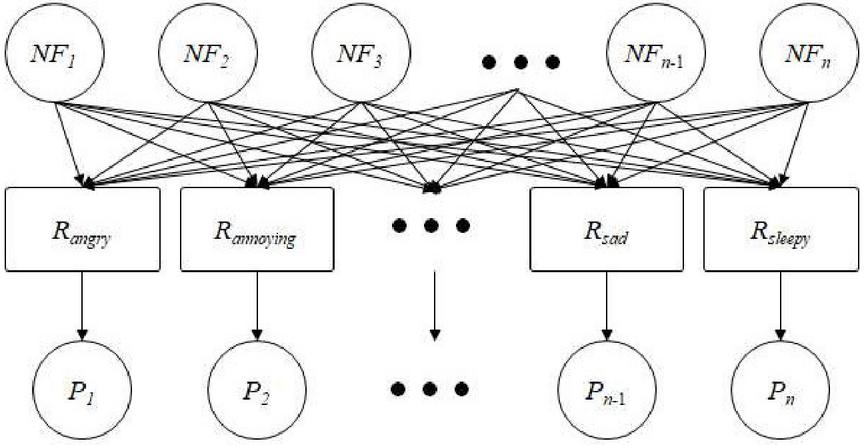
Figure 4 Structure of mood vector predictor (: the th normalized feature, : the regressor for mood , : the prediction value of mood ).
Table 2 Music–mood mapping table
| Music | Annoying | Excited | Annoying | Excited | Annoying | Excited | |||
| No. | (Intro) | (Intro) | (Representative) | (Representative) | (Outro) | (Outro) | |||
| 1 | 0.042997 | 0.14028 | 0.116106 | 0.198199 | 0.105702 | 0.112124 | |||
| 2 | -0.00057 | 0.03049 | 0.000381 | 0.125954 | 0.000381 | 0.125954 | |||
| 3 | 0.018757 | 0.107508 | 0.013017 | 0.010034 | 0.000466 | 0.057462 | |||
| 4 | 0.026859 | 0.125084 | 0.026859 | 0.125084 | 0.026908 | 0.031851 | |||
| 5 | 0.008591 | 0.046659 | 0.04826 | 0.075249 | -0.0413 | 0.009971 | |||
| 1240 | 0.134233 | 0.03463 | 0.162571 | 0.279995 | 0.065163 | 0.170485 | |||
| 1241 | -0.00236 | 0.260966 | -0.00314 | 0.151166 | 0.042663 | 0.273496 | |||
| 1242 | 0.069794 | 0.442856 | 0.054855 | 0.36362 | 0.057138 | 0.389087 | |||
| 1243 | 0.114337 | 0.412559 | 0.116601 | 0.443066 | 0.017833 | 0.380032 | |||
3.2 Creating Music Mood Vectors
To obtain the mapping information for mood tags and vectors, mood tag data for all of the music pieces used in our analysis are needed to collect. On Last.fm, listeners can check the relevant tags of a music piece (Figure 5a) or retrieve music pieces by selecting a tag. The associated music tags of a music piece are obtained automatically through API (Application Program Interface) which requires the name of the artist and the track (Figure 5b). Figure 5c gives the example of the result of the input of “Sally Shapiro” as Artist and “I’ll be by your side” as track.
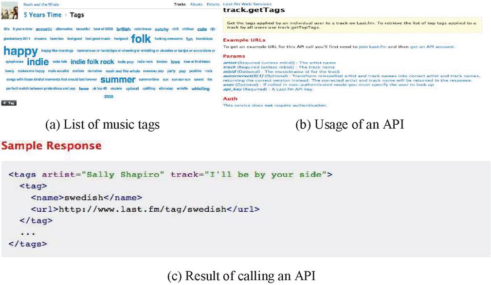
Figure 5 List of music tags on Last.fm and Usage of API.
The number of music pieces associated with each tag is shown in Table 3. As multiple tags are assigned to each piece, this number is greater than the total number of music pieces.
Table 3 Number of music pieces associated with each mood tag
| Tag | Number of Music Pieces | Tag | Number of Music Pieces |
| aggravated | 1 | calm down | 8 |
| agitated | 2 | care | 80 |
| agog | 2 | chill out | 61 |
| amused | 4 | comfort | 30 |
| angered | 1 | composed | 19 |
| Angry | 98 | console | 1 |
| Annoying | 37 | cool it | 6 |
| mellow | 440 | sad | 564 |
| mournful | 3 | Happy | 337 |
| Nervous | 33 | satisfy | 8 |
| Peaceful | 67 | settle down | 6 |
| pensive | 9 | simmer down | 3 |
| pitiful | 16 | sleepy | 43 |
Tag data and the music–mood table were used to connect mood tags and mood vectors. Only 50% 70% of tag data were used to create maps; the remaining portion was used for performance evaluation. As there are many tags for each music piece (Figure 6a), redundant tags were removed; Figure 6b depicts the outcome of this process.
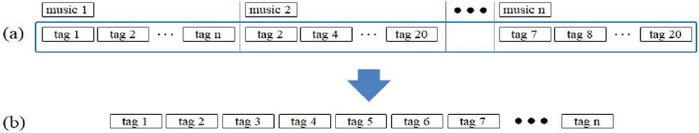
Figure 6 Removal of redundant mood tags.
Mood tables were then created (left-hand side of Figure 7), where means the mood vector of music piece with . Different numbers of music pieces were associated with each tag. Therefore, the representative mood vector of each tag needs to be defined. We did this by averaging the mood vectors for music pieces with the same tag. As each music piece has three music segments, the left-hand side of Figure 7 can be further refined into the right of Figure 7, where , and refer to the intro, representative, and outro sections, respectively, of the mood vectors of .
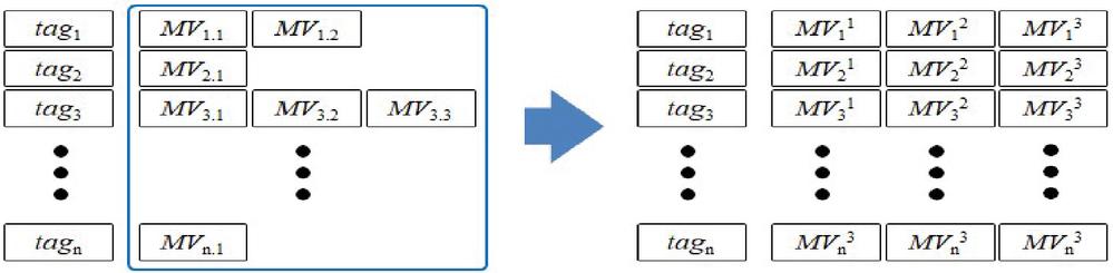
Figure 7 Creating the tag mood table of tags.
In the mood table of tags obtained from music pieces, all tags are treated as independent unless they are identical: for example, “happy” and “get happy” are treated as different tags (Table 4). But, when the retrieval performance is measured, synonyms among tags were treated as relevant (see Section 4.3).
Table 4 Tag–mood mapping table
| Annoying | Excited | Annoying | Excited | Annoying | Excited | |||||
| No. | Tag | (Intro) | (Intro) | (Representative) | (Representative) | (Outro) | (Outro) | |||
| 10 | sad | 0.036 | 0.110 | 0.054 | 0.157 | 0.053 | 0.109 | |||
| 11 | Smooth Soul | -0.024 | 0.064 | -0.003 | 0.170 | 0.001 | 0.080 | |||
| 12 | sadness | 0.073 | 0.120 | 0.035 | 0.113 | 0.050 | 0.060 | |||
| 45 | happy | 0.044 | 0.223 | 0.056 | 0.242 | 0.065 | 0.224 | |||
| 46 | get happy | 0.018 | -0.026 | 0.014 | 0.039 | 0.021 | 0.069 | |||
| 47 | always makes me happy | 0.192 | 0.268 | 0.108 | 0.229 | 0.112 | 0.204 | |||
| 419 | angry | 0.084 | 0.216 | 0.113 | 0.323 | 0.103 | 0.279 | |||
| 420 | angry hate music | 0.064 | 0.346 | 0.124 | 0.290 | 0.124 | 0.290 | |||
| 421 | angry grrrr | 0.038 | 0.263 | 0.020 | 0.257 | 0.061 | 0.254 | |||
| 424 | angry songs | 0.064 | 0.239 | 0.124 | 0.394 | 0.148 | 0.323 |
3.3 Music Retrieval Using Folksonomy Tags
The method used to retrieve music using folksonomy tags is depicted in Figure 8. First, the user inputs the tag to be retrieved (query in Figure 8). The mood vector of the query tag is then searched in the tag–mood mapping table. Then, music pieces with mood vectors similar to the mood vector of the query tag are retrieved.
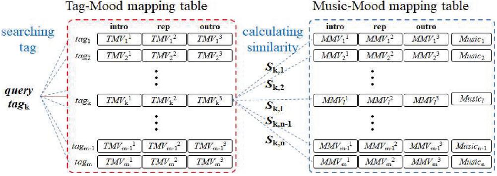
Figure 8 Music retrieval using folksonomy tags.
A calculation of cosine similarity was used to measure the similarity between two mood vectors (See Equation (3)); retrieval performance can vary depending on which mood vectors are selected. As there are three mood vectors for the three segments of each music piece, there are six possible combinations: Intro, Representative, Outro, All, 3:3 Max, and 3:1 Max. Intro searches for similarities between the first mood vector of the tag and the first mood vector of a music piece; Representative searches for similarities between the second mood vector of the tag and the second mood vector of a music piece; Outro searches for similarities between the third mood vector of the tag and the third mood vector of a music piece; All searches for similarities between all mood vectors of the tag and all mood vectors of the music piece (i.e., the tag and the music piece are both treated as 36-dimensional vectors); 3:3 MAX searches for the maximum similarities between the first, second, or third mood vectors of the tag and the first, second, or third mood vectors of a music piece; and 1:3 MAX searches for the maximum similarity between the second mood vector of the tag and all three mood vectors of a music piece. The experimental results are given in Section 4.3.
| (3) | ||
where, and mean the mood vectors of tag and music, respectively.
4 Experiments and Analysis
This section discusses three types of analysis: first, an analysis of the tag-mood table; second, a performance analysis of the prediction model used to build the music-mood table; and third, a performance analysis of music retrieval using folksonomy tags.
4.1 Analysis of the Tag-mood Table
To grasp the relationship between tags and their mood vectors in the tag-mood table, an analysis was done based on the 12 words from Thayer’s two-dimensional mood model. To this end, the 424 tags in the tag-mood table were classified into 12 groups; each group corresponds to one of Thayer’s 12 words (Table 5). For example, the tag “always makes me happy” is classified as happy and the tag “Elton john, sad songs” is classified as sad. Tags containing two moods like “happy sad” are classified as both groups.
Table 5 Grouping of tags into Thayer’s 12 mood categories
| Annoying | Angry | Nervous |
| “all things annoying in the world put together into one”, “annoying”, “not annoying”, and 1 other | “8 angry”, “a bit angry”, “aaaangry”, “angry”, “angry afternoon”, and 32 others | “nervous”, “nervousbreakdown” |
| sad | bored | sleep |
| “a sad weightlessness”, “alkiviadis sadness”, “Angst and Sadness”, “another sad love song”, and 186 others | “bored”, “bored to death”, “boredom”, “get bored”, and 6 others | “makes you sleepy without being boring”, “sleepy”, “sleepy baby”, “sleepy music”, “sleepy song”, and 8 others |
| calm | peaceful | relaxed |
| “Beth Orton verde si calm”, “calm”, “calm and nice”, “calm country”, “calm down”, and 27 others | “Peaceful Sounds”, “Peacefulspot”, “calm-peaceful”, “peaceful” | “relaxed”, “relaxed not bored”, “relaxed piano”, “relaxed rock”, “warm soft relaxed” |
| pleased | happy | excite |
| “pleased” | “always makes me happy”, “be happy dammit”, “becks happy songs”, “bright and happy”, “catchy happy”, and 117 others | “Shivering Excitement”, “excite”, “excite me”, “the word excite” |
One-way analysis of variance (ANOVA) testing was performed to check if the mood distributions of the 12 categories were mutually independent. The independent variables for the ANOVA test were Thayer’s 12 mood tags (happy, sad, annoying, pleased, excited, nervous, bored, sleepy, calm, peaceful, relaxed, angry) and the dependent variables were the mood vectors. Results are shown in Table 6; all p-values are 0.000. This means that the null hypothesis () can be rejected and the alternative hypothesis () supported, thus indicating that the distributions of mood vectors are affected by mood tags.
Table 6 One-way analysis of variance testing to prove mutual independence of Thayer’s 12 mood categories
| Mood | Annoying | Angry | Nervous | Sad | ||||||||
| Section | I | R | O | I | R | O | I | R | O | I | R | O |
| DF | 11 | 11 | 11 | 11 | 11 | 11 | 11 | 11 | 11 | 11 | 11 | 11 |
| F | 12.95 | 18.19 | 13.09 | 11.31 | 15.7 | 12.68 | 6.56 | 8.81 | 7.62 | 7.64 | 9.87 | 7.29 |
| P | 0.000 | 0.000 | 0.000 | 0.000 | 0.000 | 0.000 | 0.000 | 0.000 | 0.000 | 0.000 | 0.000 | 0.000 |
| Mood | Bored | Sleepy | Calm | Peaceful | ||||||||
| DF | 11 | 11 | 11 | 11 | 11 | 11 | 11 | 11 | 11 | 11 | 11 | 11 |
| F | 13.95 | 14.31 | 12.91 | 15.77 | 16.04 | 17.15 | 14.17 | 16.22 | 17.15 | 8.33 | 14.73 | 13.74 |
| P | 0.000 | 0.000 | 0.000 | 0.000 | 0.000 | 0.000 | 0.000 | 0.000 | 0.000 | 0.000 | 0.000 | 0.000 |
| mood | Relaxed | Pleased | Happy | Excited | ||||||||
| DF | 11 | 11 | 11 | 11 | 11 | 11 | 11 | 11 | 11 | 11 | 11 | 11 |
| F | 9.67 | 16.02 | 12.17 | 10.13 | 6.72 | 6.66 | 7.81 | 5.13 | 3.95 | 10.17 | 12.4 | 12.76 |
| P | 0.000 | 0.000 | 0.000 | 0.000 | 0.000 | 0.000 | 0.000 | 0.000 | 0.000 | 0.000 | 0.000 | 0.000 |
| Note. I Intro, R Representative, O Outro, DF Degrees of Freedom, F F-value, P P-value. | ||||||||||||
4.2 Analysis of SVR Performance
To select the parameters of the predictors in Figure 3 with the best performance, 281 music segments from Moon et al.’s dataset [14] were grouped into 10 groups for 10-fold Cross Validation, in which nine groups were used for training and one group for testing. The parameter C was increased from 1 to 100 by increments of 5, and the parameter was increased from 0.1 to 1.0 by increments of 0.1. For all moods, the performance of nu-SVR was better than epsilon-SVR [24]. The performance of the RBF kernel was better than other kernels for annoying, excited, and nervous; the sigmoid kernel was better than the other kernels for relaxed; and the polynomial kernel was better than the other kernels for all other moods (Table 7).
Table 7 Single vector regression performance for Thayer’s 12 moods
| Mood Value | SVR | Kernel | nu | C | Squared Correlation |
| annoying | nu | radial basis function | 0.6 | 1 | 0.53 |
| angry | polynomial | 0.1 | 22 | 0.54 | |
| nervous | radial basis function | 0.4 | 1 | 0.37 | |
| sad | polynomial | 0.9 | 19 | 0.37 | |
| bored | polynomial | 0.7 | 2 | 0.30 | |
| sleepy | polynomial | 0.3 | 3 | 0.51 | |
| calm | polynomial | 0.8 | 6 | 0.71 | |
| peaceful | polynomial | 0.1 | 19 | 0.76 | |
| relaxed | sigmoid | 0.3 | 1 | 0.52 | |
| pleased | polynomial | 1 | 5 | 0.32 | |
| happy | polynomial | 0.2 | 17 | 0.38 | |
| excited | radial basis function | 0.2 | 2 | 0.67 |
4.3 Analysis of Retrieval Performance by Folksonomy Tags
Although all mood words could be used as query tags to measure the retrieval performance of the suggested method, only the 12 words from Thayer’s two-dimensional mood model were considered due to the limitations on processing such a vast data set. Synonyms (provided by www.synonym.com) were used to build the answer set for the 12 mood words (Table 8); For example, the tag “peaceable” was grouped with “peaceful,” as “peaceable” is a synonym of the basic mood adjective “peaceful.” The answer built in this method is given in Table 9 where No. refers to the numerical identifier of each of the 1,375 music pieces used in the analysis. Scores are given as “0” if the mood is not present or “1” if the mood is present for a given music piece. Each music piece had at least one mood tag; the number of music pieces associated with each mood are calm (501), pleased (241), sad (527), excited (304), nervous (151), peaceful (90), relaxed (527), happy (290), bored (190), sleepy (79), angry (205), and annoying (242) (Table 9).
Table 8 Example synonyms for Thayer’s 12 moods
| Mood | Annoying | Angry | Nervous | Sad |
| verb | annoy, rag, get to, bother, and 10 others | – | – | – |
| adj | bothersome, galling, irritating, and 10 others | aggravated, provoked, angered, enraged, and 25 others | tense, anxious, queasy, uneasy, unquiet, and 6 others | bittersweet, doleful, mournful, heavyhearted, and 15 others |
| mood | bored | sleepy | calm | peaceful |
| verb | bore, tire, drill, cut | – | calm down, tranquilize, tranquillise, quieten, lull, and 15 others | – |
| adj | world-weary, tired, blase, uninterested | sleepy-eyed, sleepyheaded, asleep(predicate) | unagitated, serene, tranquil, composed, placid, and 6 others | peaceable, irenic, nonbelligerent, pacific, and 4 others |
| mood | relaxed | pleased | happy | excited |
| verb | relax, loosen, loosen up, unbend, and 17 others | please, delight, satisfy, gratify, wish, and 2 others | – | excite, arouse, elicit, enkindle, kindle, evoke, fire, and 28 others |
| adj | degage, laid-back, mellow, unstrained | amused, diverted, entertained, encouraged, and 6 others | blessed, blissful, bright, golden, riant, felicitous, and 6 others | aroused, emotional, worked up, agitated, and 18 others |
| Note. Synonyms obtained from www.synonym.com | ||||
Table 9 Measuring retrieval performance using Thayer’s 12 mood tags
| No. | Calm | Pleased | Sad | Excited | Nervous | Peaceful | Relaxed | Happy | Bored | Sleepy | Angry | Annoying |
| 1 | 0 | 1 | 0 | 0 | 0 | 0 | 1 | 0 | 0 | 1 | 0 | 0 |
| 2 | 0 | 0 | 0 | 0 | 0 | 1 | 0 | 0 | 0 | 0 | 0 | 0 |
| 3 | 0 | 0 | 0 | 1 | 0 | 0 | 0 | 0 | 0 | 0 | 1 | 0 |
| 4 | 1 | 0 | 0 | 0 | 0 | 0 | 0 | 0 | 0 | 1 | 0 | 0 |
| 5 | 0 | 0 | 0 | 0 | 0 | 0 | 0 | 1 | 0 | 0 | 0 | 0 |
| 6 | 0 | 0 | 0 | 0 | 0 | 0 | 1 | 0 | 0 | 0 | 0 | 0 |
| 7 | 0 | 0 | 1 | 0 | 0 | 0 | 0 | 0 | 0 | 0 | 0 | 0 |
| 8 | 0 | 0 | 0 | 0 | 0 | 0 | 1 | 0 | 1 | 0 | 1 | 0 |
| 9 | 0 | 0 | 1 | 0 | 0 | 0 | 0 | 0 | 0 | 0 | 0 | 0 |
| 10 | 0 | 0 | 0 | 1 | 0 | 0 | 0 | 0 | 0 | 0 | 0 | 0 |
| 1371 | 0 | 0 | 0 | 0 | 0 | 1 | 0 | 0 | 0 | 0 | 0 | 0 |
| 1372 | 0 | 0 | 0 | 0 | 0 | 1 | 1 | 0 | 0 | 0 | 0 | 0 |
| 1373 | 0 | 0 | 0 | 0 | 0 | 1 | 0 | 0 | 0 | 0 | 0 | 0 |
| 1374 | 0 | 0 | 0 | 0 | 0 | 1 | 0 | 0 | 0 | 0 | 0 | 1 |
| 1375 | 0 | 0 | 0 | 1 | 0 | 1 | 0 | 0 | 0 | 0 | 0 | 0 |
| Total | 501 | 241 | 527 | 304 | 151 | 90 | 527 | 290 | 190 | 79 | 205 | 242 |
The retrieval performance for the six combinations of mood vectors is given in Figure 8. The results in Figure 9 come from using 50% of the music pieces in Table 9 to build the tag-mood table, and using the other 50% of the music pieces in Table 9 for testing. The best performance at recall level 0.1 was 0.49 for Intro, 0.59 for Representative, 0.50 for Outro, 0.54 for All, 0.51 for 3:3 MAX, and 0.56 for 1:3 MAX; Representative performed the best at most recall levels (Figure 9).
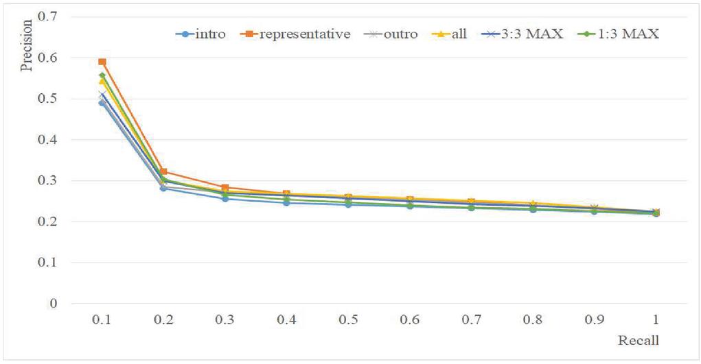
Figure 9 Retrieval performance for the six combinations of mood vectors (Ratio of training: testing data 50:50; 12 moods).
The number of musical pieces associated with given mood tags varied (Table 9); we hypothesized that tags associated with few music pieces might adversely affect overall performance. To check this hypothesis, we repeated the analysis using only the eight moods associated with at least 190 musical pieces each. Retrieval performance at all recall levels was improved by approximately 0.05; the best performance (0.65) was achieved for Representative at recall level 0.1 (Figure 10).
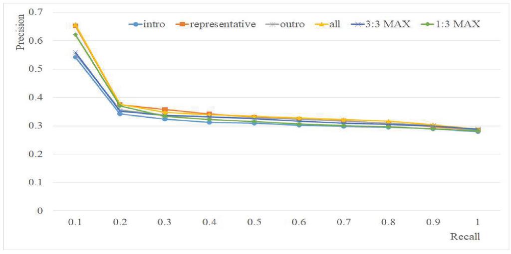
Figure 10 Retrieval performance for the six combinations of mood vectors (Ratio of training: testing data 50:50; 8 moods).
From the results presented in Figure 10, we can conclude that the performance of the method suggested in the present paper will likely be improved if more music pieces are used to build the tag-mood table. To test this hypothesis, the ratio of training is changed from 50:50 to 70:30. With this new ratio, best performance was improved by 0.05 (from 0.59 to 0.64) using 12 moods, and improved by 0.08 (from 0.65 to 0.73) using 8 moods (Figure 11).
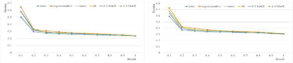
Figure 11 Retrieval performance for the six combinations of mood vectors (Ratio of training: testing data 70:30).
Table 10 The retrieval performance of the keyword-based method
| Number of Music | Number of Music | ||
| Tags | with Synonym | Without Synonym | Recall |
| calm | 501 | 171 | 0.37 |
| Pleased | 241 | 3 | 0.01 |
| sad | 527 | 303 | 0.62 |
| Excited | 304 | 38 | 0.14 |
| Nervous | 151 | 33 | 0.25 |
| peaceful | 90 | 67 | 0.99 |
| Relaxed | 527 | 102 | 0.22 |
| happy | 290 | 208 | 0.77 |
| Bored | 190 | 37 | 0.23 |
| sleepy | 79 | 56 | 0.76 |
| Angry | 205 | 75 | 0.38 |
| Anooying | 242 | 26 | 0.11 |
| Average Recall | 0.36 | ||
4.4 Comparing Retrieval Performance the Keyword Based Method and the Proposed Method
The recall of the keyword-based method was shown in Table 10. Its precision was 1.0 because only songs having the exactly matched tag are retrieved. The recall of the ‘happy’ tag was 0.77, which was a case where the number of songs including the synonym tag was about 23%. The recall of the tag ‘Pleased’ was 0.01 because the number of songs including the tag ‘Pleased’ was three. Therefore, only three songs can be provided as a retrieval result. Nevertheless, the precision of the proposed method may be lower than the keyword-based, but more music can be provided as a retrieval result in the case of using the ‘Pleased’ tag because synonyms were considered.
The retrieval performance of the ‘happy songs’ tag and the ‘sad songs’ tag was also compared as shown in Table 11. The result showed the best performance when the cosine similarity was applied to the AV value. Their precisions were 0.81 and 0.94 at the recall of 0.1. However, the precision of the keyword-based method was 1.0, but when synonyms were considered, recalls were 0.04 (11/290) for the “happy songs” tag and 0.09 (49/527) of the “sad songs” tag. This imply that the keyword-based method shows good performance in precision but has a disadvantage in that songs having similar mood but different tags cannot be retrieved.
Table 11 Retrieval performances of the keyword-based method and the proposed method
| ‘Happy Songs’ Tag | ‘Sad Songs’ Tag | |||
| Recall | Proposed | Keyword-based | Proposed | Keyword-based |
| Level | Method | Method | Method | Method |
| 0.1 | 0.81 | 1.00 (11/290) | 0.94 | 1.00 (49/527) |
| 0.2 | 0.38 | 0.59 | ||
| 0.3 | 0.35 | 0.59 | ||
| 0.4 | 0.32 | 0.58 | ||
| 0.5 | 0.29 | 0.56 | ||
| 0.6 | 0.27 | 0.52 | ||
| 0.7 | 0.27 | 0.50 | ||
| 0.8 | 0.26 | 0.46 | ||
| 0.9 | 0.25 | 0.45 | ||
| 1 | 0.23 | 0.43 |
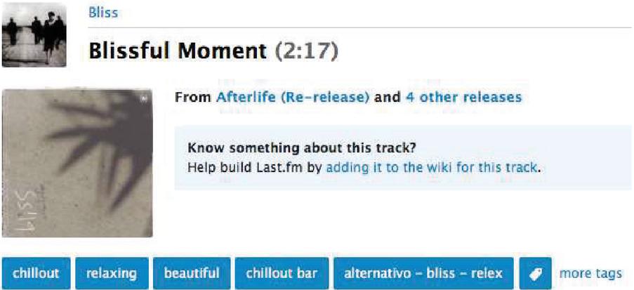
Figure 12 Music containing ‘relex’ tag in last.fm.
Some of the typos were included in folksonomy tags, and those typos can be treated as a new word. In this paper, to check whether music retrieval was possible when using typos of tags, retrieval performance was identified using the ‘relex’ tag in last.fm. The ‘relex’ tag has not been registered in the English-English dictionary. As you can see from Figure 12, perhaps the user has entered ‘relax’ tag incorrectly. Anyway, in the keyword-based method, songs having the corrected tag of typos cannot be retrieved. But, as shown in Figure 13, songs having “relax” tag were recommended in the proposed method when searching with “relex” tag.
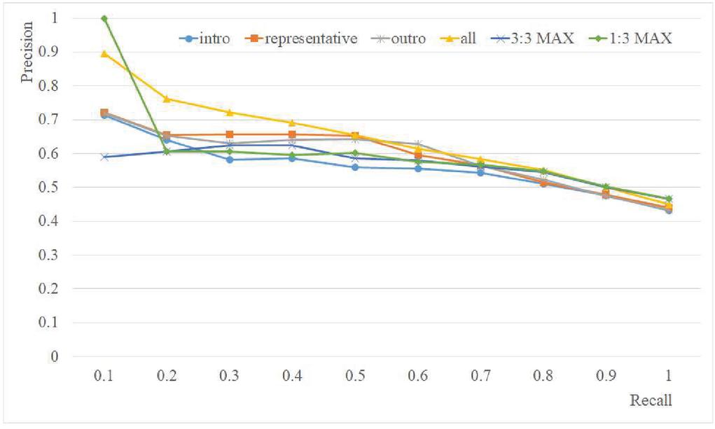
Figure 13 Retrieval performance by the ‘relex’ tag.
5 Conclusion
To solve the synonym problem associated with folksonomies, the mood vector of music was introduced as an internal tag. A mood vector consists of 12 values indicating the presence of the 12 moods from Thayer’s two-dimensional mood model. Music pieces were tagged internally using these numeric values, enabling the retrieval of music with similar moods. To implement a retrieval system based on internal tags, music vectors must be generated for both music pieces and folksonomy tags.
The music vector of a given music piece was generated by 12 regressors, each of which predicts the possibility of a given mood in that music piece. These regressors were built using SVR of LIBSVM and their parameters showing good performance are searched through lots of experiments. The music vector of a folksonomy tag was determined by averaging the mood vectors of music pieces having the tag in the training data set. In our experiments, the dataset consisting of music pieces having at least one mood tag in Last.fm and their mood tags was used; part of the dataset was used as the training set and the remainder of the dataset was used as the testing set. To check if mood vectors of tags obtained by the method were meaningful (i.e., to confirm a statistically significant association between mood vectors and folksonomy tags) ANOVA tests were performed. The results show that the mood vectors of music have different distributions for the 12 mood tags; mood vectors of tags are therefore at least somewhat meaningful.
The present paper demonstrated the internal tagging of music to be quite useful when combined with our approach for solving the problem caused by synonyms. However, the retrieval performance of our approach could be improved by enhancing the predictive power of mood vectors, which is largely dependent on the quality and quantity of the training data provided. In the present paper, the training data were collected from university students in the engineering department; data collected from musicians or students majoring in music would be expected to improve performance by improving data quality. Obtaining more tagging data would also be expected to improve performance (as illustrated in Section 4.3).
Acknowledgments
This research was supported by Basic Science Research Program through the National Research Foundation of Korea (NRF) funded by the Ministry of Education (NRF-2020R1F1A104833611, 2021R1I1A1A01042270).
References
[1] J. A. Russell, ‘A Circumplex Model of Affect’, Journal of Personality and Social Psychology, 39(6), pp. 1161–1178, 1980.
[2] K. Hevner, ‘Experimental studies of the elements of expression in music’, The American Journal of Psychology, 48(2), 246–268, 1936.
[3] R. E. Thayer, ‘The Biopsychology of Mood and Arousal’, Oxford University Press, 1989.
[4] D. Liu, N. Zhang and H. Zhu, ‘Form and mood recognition of Johann Strauss’s waltz centos’, Chinese Journal of Electronics, 12(4), 2003.
[5] H. Katayose, M. Imai and S. Inokuchi, ‘Sentiment extraction in music’, Proceedings of the 9th International Conference on Pattern Recognition, pp. 1083–1087, 1988.
[6] Y. Feng, Y. Zhuang and Y. Pan, ‘Popular Music Retrieval by Detecting Mood’, Proceedings of the 26th annual international ACM SIGIR conference on Research and development in informaion retrieval, pp. 375–376, 2003.
[7] T. Li and M. Ogihara, ‘Detecting emotion in Music’, ISMIR, 3, pp. 239–240, 2003.
[8] K. Hevner, ‘Expression in music: a discussion of experimental studies and theories’, Psychological Review, 42(2), pp. 186–204, 1935.
[9] P. R. Farnsworth, ‘The Social Psychology of Music’, The Dryden Press, 1958.
[10] Y. H. Yang, C. C. Liu and H. H. Chen, ‘Music emotion classification: a fuzzy approach’, Proceedings of the 14th Annual ACM International Conference on Multimedia, pp. 81–84, 2006.
[11] Y. H. Yang, Y. F. Su, Y. C. Lin and H. H. Chen, ‘Music emotion recognition: the role of individuality’, Proceedings of the International Workshop on Human-centered Multimedia, pp. 13–22, 2007.
[12] Y. H. Yang, C. C. Liu and H. H. Chen, ‘A regression approach to music emotion recognition’, IEEE Transactions on Audio Speech and Language Processing, 16(2), pp. 448–457, 2008.
[13] J. I. Lee, D. G. Yeo, B. M. Kim and H. Y. Lee, ‘Automatic Music Mood Detection through Musical Structure Analysis’, International Conference on Computer Science and its Application, pp. 510–515, 2009.
[14] C. B. Moon, H. S. Kim, H. A. Lee and B. M. Kim, ‘Analysis of relationships between mood and color for different musical preferences’, Color Research & Application, 39(4), pp. 413–423, 2014.
[15] S. R. Ness, A. Theocharis, G. Tzanetakis and L. G. Martins, ‘Improving Automatic Music Tag Annotation Using Stacked Generalization Of Probabilistic SVM Outputs’, Proceedings of the 17th ACM International Conference on Multimedia, pp. 705–708, 2009.
[16] C. Laurier, M. Sordo, J. Serra and P. Herrera, ‘Music Mood Representation from Social Tags’, ISMIR, pp. 381–386, 2009.
[17] J. H. Kim, S. Lee, S. M. Kim and W. Y. Yoo, ‘Music mood classification model based on Arousal-Valence values’, Advanced Communication Technology (ICACT), 2011 13th International Conference on, pp. 292–295, 2011.
[18] M. Levy, M. Sandier and M. Casey, ‘Extraction of High-Level Musical Structure From Audio Data and Its Application to Thumbnail Generation’, Acoustics, Speech and Signal Processing, 2006. ICASSP 2006 Proceedings. 2006 IEEE International Conference on, 5, pp. 13–16, 2006.
[19] O. Lartillot and P. Toiviainen, ‘A Matlab toolbox for musical feature extraction from audio’, International Conference on Digital Audio Effects, pp. 237–244, 2007.
[20] S. J. Ryu, H. Y. Lee, I. W. Cho and H. K. Lee, ‘Document Forgery Detection with SVM Classifier and Image Quality Measure’, Advances in Multimedia Information Processing-PCM 2008, pp. 486–495, 2008.
[21] C. C, Chang and C. J. Lin, ‘LIBSVM: a library for support vector machines’, ACM Transactions on Intelligent Systems and Technology (TIST), 2(3), p. 27, 2011.
[22] E. D. Scheirer, ‘Music-listening Systems’, Ph. D. Thesis, MIT Media Lab, 2000.
[23] Y. E.. Kim and W. Brian, ‘Singer Identification in Popular Music Recordings Using Voice Coding Features’, Proceedings of the 3rd International Conference on Music Information Retrieval, 13, 17, 2002.
[24] Seungmin Rho, Byeong-jun Han and Eenjun Hwang, ‘SVR-based music mood classification and context-based music recommendation’, Proceedings of the 17th International Conference on Multimedia 2009, Vancouver, British Columbia, Canada, October 19–24, 2009.
[25] C. B. Moon, J. Y. Lee, D. S. Kim and B. M. Kim, ‘Multimedia content recommendation in social networks using mood tags and synonyms’, Multimedia Systems 26, 139–156 (2020).
Biographies

Chang Bae Moon received a BSc, an MSc, and a PhD from the Dept. of Software Eng. at Kumoh National Institute of Technology, Korea, in 2007, 2010, and 2013, respectively. He has been with the Kumoh National Institute of Technology since 2014 as a Research Professor in the ICT Convergence Research Center. From 2013 to 2014, he was a Senior Researcher in Young Poong Elec. Co. His current research areas include artificial intelligence, Web intelligence, information filtering, and image processing.

Jong Yeol Lee received the BS and MS degree in Dept. of computer Eng. from Kumoh National Institute of Technology, Korea, in 1992 and 1994, respectively and the PhD candidate in software Eng. from Kumoh National Institute of Technology, Korea, in 2018. He has been with Kumoh National Institute of Technology since 2005 as a time lecturer of Computer Software Engineering Department. His current research areas include Artificial Intelligence, Machine Learning and Information Security.

Byeong Man Kim received the BS degree in Dept. of computer Eng. from Seoul National University (SNU), Korea, in 1987, and the MS and the PhD degree in computer science from Korea Advanced Institute of Science and Technology (KAIST), Korea, in 1989 and 1992, respectively. He has been with Kumoh National Institute of Technology since 1992 as a faculty member of Computer Software Engineering Department. From 1998–1999, he was a post-doctoral fellow in UC, Irvine. From 2005–2006, he was a visiting scholar at Dept. of Computer Science of Colorado State University, working on design of a collaborative Web agent based on friend network. His current research areas include artificial intelligence, Web intelligence, information filtering and brain computer interface.
Journal of Web Engineering, Vol. 20_8, 2335–2360.
doi: 10.13052/jwe1540-9589.2086
© 2021 River Publishers