Few-shot Text Classification Method Based on Feature Optimization
Jing Peng1,* and Shuquan Huo2
1School of Philosophy, Anhui University, Hefei, 230039, China
2School of Philosophy and Public Management, Henan University, Kaifeng, 475004, China
E-mail: pjgoodluck@126.com
*Corresponding Author
Received 16 December 2022; Accepted 12 April 2023; Publication 04 July 2023
Abstract
For the poor effect of few-shot text classification caused by insufficient data for feature representation, this paper combines wide and deep attention bidirectional long short time memory (WDAB-LSTM) and a prototypical network to optimize text features for better classification performance. With this proposed algorithm, text enhancement and preprocessing are firstly adopted to solve the problem of insufficient samples and WDAB-LSTM is used to increase word attention to get output vectors containing important context-related information. Then the prototypical network is added to optimize the distance measurement module in the model for a better effect on feature extraction and sample representation. To test the performance of this algorithm, Amazon Review Sentiment Classification (ARSC), Text Retrieval Conference (TREC), and Kaggle are selected. Compared with the Siamese network and the prototypical network, the proposed algorithm with feature optimization has a relatively higher accuracy rate, precision rate, recall rate, and F value.
Keywords: Few-shot learning, text classification, feature optimization, WDAB-LSTM prototypical network.
1 Introduction
Although great achievements have been obtained in text classification with traditional methods relying on a large amount of data to pretrain language models, it is not so satisfactory when there is not sufficient data for feature extraction as the task requires [1–3]. Hence few-shot text classification, which concerns learning from limited data samples for useful features, and processing them is still a research topic [4–6]. The common few-shot text classification algorithms in this article include memory networks, meta-learning, Bayesian calculations, and measurement.
A memory network is often used for few-shot text classification. Its main idea is to extract relevant knowledge from data and store it in external storage in the form of key-value [7-9]. When forecasting the samples in the query set, relevant keys are found for corresponding values according to information on the query object. Santoro [10], Geng [11], etc. used memory networks to help classification models learn from new data to complete few-shot text classification tasks. Although the memory network provides more effective information for the model, it requires large storage space.
Meta-learning, another method commonly used in recent years, learns from data with known tags for their distribution. It is advantageous in generalization and task adaptation [12–14]. Munkhdalai [15] and Yu et al. [16] used this method to enhance the generalization ability of classification models for better classification effects. However, large numbers of parameters, slow convergence speed, and high complexity turn out to be its shortcomings.
For few-shot text classification algorithms, besides the convergence speed and classification accuracy, the uncertainty of the algorithm also needs to be considered [17–20]. Bayesian inference can solve this problem and it can improve the robustness of the algorithm. Yoon et al. [21] proposed a model-agnostic meta-learning (MAML) method based on the Bayesian model to reduce the uncertainty of the algorithm by fitting the posterior distribution of parameters. However, this method needs a long time and a large space for model training.
In order to reduce the complexity of the algorithm for the convenience of calculation and optimization, scholars have studied a few-shot text classification method based on measurement which extracts features of the samples to build an appropriate feature space and model the distance between samples to obtain a function through learning to measure the similarity based on the principle of same-near and different-far to predict the classification of unlabeled data [22–24]. Snell [25], Li [26], etc. improved the generalization ability of the model by calculating the distance between the query objects and each classification prototype in the support set. However, the method based on the measurement is sensitive to sample size. When there are insufficient samples, a wrong selection of measurement function will affect the performance of the model.
Based on the analysis of relevant technologies and algorithms for few-shot text classification, this paper proposes a method combining wide and deep attention bidirectional long short time memory (WDAB-LSTM) and a prototypical network. This algorithm underlines two aspects: sample size and feature optimization. For the former, text enhancement and preprocessing are needed in the face of insufficient samples. For the latter, WDAB-LSTM and a prototypical network are used to optimize the model in context-relatedness and vector distance measurement so as to promise a lower sensitivity of the algorithm to samples and thus improve classification performance. The performance of the proposed algorithm is tested with the classic few-shot text classification dataset Amazon Review Sentiment Classification (ARSC), Text Retrieval Conference (TREC), and Kaggle, and compared with the Siamese neural network and prototypical neural network. Experimental results show that the proposed network performs better in accuracy, precision, recall, F value, and errors rate.
2 Text Preprocessing for Few-shot Classification
To solve the problem of insufficient samples in the data set, text enhancement and preprocessing should be conducted to increase the number of samples before classification.
2.1 Text Enhancement Based on EDA and Back Translation
This paper uses easy data augmentation (EDA) and back translation for text enhancement. After text enhancement, the number of samples in the dataset can be significantly increased, which is helpful for model parameters through training and alleviates the overfitting of few-shot learning models.
EDA [27] includes the following four methods:
Synonym replacement: x words are randomly sampled from the input sample sequence and then replaced by their synonyms randomly selected from the corresponding synonym set. For example, “This book is so interesting that I read it all day.” becomes “This book is so entertaining that I read it all day.” after replacement.
Random insertion: Randomly sample a word from the input sample sequence and select a position in the original input sample sequence to place its synonym.
Random exchange: Exchange two words randomly selected in the input sample sequence.
Random deletion: Based on experience and sample sequence length, set the proportion of words that can be deleted in the sample sequence. Randomly delete words from the input sample sequence at the set certain proportion. For example, “This book is so interesting that I read it all day.” becomes “book is so interesting I read it all day.” after random deletion.
These processes are completed and the text is further enhanced by a back translation which translates sample data into an intermediate language and then from the intermediate language back to the original language. This is a common technique for text enhancement. After back translation, new sample data with the same meaning as the original ones in different expressions will be obtained. Compared with the original data, it is likely that the new sample data changed in sentence structure will have some words obtained such as the synonyms of the original words or the deleted ones from back translation.
2.2 Text Preprocessing
Text preprocessing comes after text enhancement. In this experiment, Stanford’s Global Vectors for Word Representation (GloVe) whose total size is 1.75GB from the training of the super large dataset Common Crawl is used [28]. The dimension of the pre-training word embedding is 300. After the word list is obtained, the text in the dataset is preprocessed as follows:
1. Deactivated words such as “a” and “to” are deleted when training the GloVe word embedding, so these words are removed from the experimental training set data in this paper.
2. Some special symbols, including “$?!., #% () *+-/:;=”, etc. are removed.
3. For numbers, all those greater than 9 in the pre-training word embeddings are replaced by “#”. For example, “123” becomes “# # #” and “15.80” becomes “# #. # #”.
Finally, the cleaned dictionary (glossary) is used as the experimental input, which is a matrix of word embeddings composed of those selected from the dictionary.
3 Strategy for Few-shot Text Classification
The WDAB-LSTM prototypical network model proposed in this paper is shown in Figure 1. This model represents categories in the dataset as vectors and then the distance between these vectors and those of the new samples is calculated, where the nearest one decides which category the new samples should fall into.
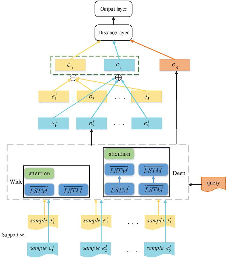
Figure 1 WDAB-LSTM prototypical network model.
The calculation of the model is based on data contained in the support set. Each classification is calculated by the vector representation of its corresponding sample data with an average value. In the testing phase of the network, the prediction sample data is mapped to a sample space of equal size to calculate the distance between the new sample space and the existing classification vectors. The classification vector with the smallest distance value is taken as the classification of the prediction sample [29, 30]. A certain type of sample is put into the wide and deep encoder for the vectorization of each sample. The wide and deep encoder consists of a wide network and a deep network. The wide network is a single-layer aBi-LSTM network that uses a bidirectional LSTM model to extract contextual information from text. Samples are output in the wide network either directly through back-to-front LSTM or through front-to-back LSTM and attention layers. This one is the attention layer used to extract the importance and connections between words. The deep network part is a two-layer aBi-LSTM network that extracts contextual information from text. The samples are output in the deep network either directly through back-to-front LSTM or through two layers of front-to-back LSTM and attention layers. This attention layer is consistent with the attention layer in the wide network architecture, which is used to extract the importance and connections between words. In this way, the model can focus on both important semantic information and all words in the sentence. The output of the wide and deep encoder is vectorized using Equation (1). Then, the representation of the class is to be obtained by summing the vectors of each sample, as shown in Equation (2). The vectorization of each sample is obtained by putting samples in the query set into the editor, as shown in Equation (3). A function is given to calculate the distance with the representation of each classification in the support set, as shown in Equation (4). The label of the class with the smallest distance is the output value of the sample, as shown in Equation (5). Finally, the WDAB-LSTM prototypical network uses the Euler formula under Bregman divergence to calculate the distance between different vectors, that is, the distance between class vectors and sample vectors, as shown in Equations (6), and (7).
| (1) |
where represents the ith sample, represents the embedded function, that is, the sample is vectorized by WDAB-LSTM, and represents the vectorized representation of sample .
| (2) |
where is the vectorized representation of the class.
| (3) |
Where represents a sample in the query set and represents the vectorization of this sample.
| (4) | |
| (5) |
where is the distance between the query set sample and class , is the predictive value of the model and it is the label of the class to which the minimum value belongs.
| (6) | |
| (7) |
where represents Bregman divergence; is a strictly differentiable convex function; , represents two vectors; is the gradient; represents the square of the Euclidean distance between and .
4 Experimental Results and Analysis
4.1 An Introduction to the Data Set
This paper uses the classic dataset, ARSC, provided by the Amazon platform [32] for few-shot text classification. ARSC includes 23 kinds of review data, each coming from Amazon users’ comments on, and star selection, for goods sold. All products are thus graded according to the review data above. “Graded” refers to the classification of products according to their star selection (0–5 stars), which includes t5 (5 stars), t4 (3–4 stars), and t2 (0–2 stars), as shown in Figure 2.
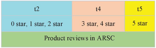
Figure 2 Three tasks divided according to star rating of comments.
The ARSC dataset contains 69 (23 3) task data. Its sample data and categories are shown in Table 1. As there are different pieces of comment on each product in the original data, the imbalance of sample size for different tasks asks for new construction of the original data set by selecting data for each task according to the proportion of the number of comments so that the data of each task can be balanced. The final data set uses 12 tasks (including three secondary tasks of books, DVDs, electronic products, and kitchen products) as the test set and the remaining 57 tasks as the training set.
Table 1 Sample and classification examples of ARSC
| Sample Examples | Classification Example |
| “i saw this pair shoes thought they very cute, however, when they arrived they smalls stains over front shoe.” | apparel. t2 |
| “i liked boots first couple weeks-they very warm comfy, however they not all durable-after month use soles holes.” | apparel. t4 |
| “it golden color very remarkable.. it looks like real gold.. wonderful piece” | apparel. t5 |
| “if you tinted windows this product not work” | automotive. t2 |
| “i purchased it year half ago. It still job. However, I recently noticed duster not work well beginning” | automotive. t4 |
| “works great! Use it around house, computer monitors, tvs, your car dash, etc.” | automotive. t5 |
| “i not impressed. It smells just like ordinary soap-so what?” | beauty. t2 |
| “i used sample liked fact it cleaned my hair way I want my hair cleaned.” | beauty. t4 |
| “i bought entire line products lisa hair regimen carol daughter website.” | beauty.t5 |
The length of the experimental sample sequence is limited to 100. C-way K-shot is used for model training, i.e. one episode is constructed for each training to calculate the gradient and update the parameters of the model. For each episode, C kinds of data are randomly selected from the training data set, and from each class K samples are randomly chosen for a total number of to form a labeled reference data set, namely, the support set. The remaining samples from the C-type are used as query sets. To train the model, it is supposed to learn from the given support set to minimize the loss value of the query set. In the experiment, a two-way five-shot is selected for the training and testing of the model. The input is five samples of a certain classification in the support set, each episode having two classifications with a total of 10 samples.
4.2 Model Training
The training of the WDAB-LSTM prototypical network uses the algorithm below, in which means the training set of the model, x represents the input of the model, y represents the tag, represents the predictive value and W represents the model parameter.
The LazyAdam is used to optimize the function of cross entropy loss in the training of the WDAB-LSTM prototypical network model. Since the C-way K-shot method trains to build an episode each time to calculate the gradient and update the model parameters and there are very limited samples, only a small number of vectors corresponding to the gradient is non-zero when updating parameters for each episode of the model. Thus, the LazyAdam optimizer is needed to process gradient updating for sparse variables to alleviate the overfitting of few-shot models.
Algorithm: WDAB-LSTM prototypical network training
1:
2:
3: for Episode do
4: Randomly select classes from
5: Select K samples from each class to obtain a support set
6: The remaining samples in classes form a query set
7: Send the support set S to the coding layer to obtain the vectorized representation of each sample
8: Sum the sample vectors in E to obtain the vectorized representation of the class
9: Send the samples in the query set Q to the coding layer to obtain a vectorized representation
10: Calculate the square of the Euclidean distance between various vectors in T and
11: The class label with the minimum distance is the predicted value output of the query sample vector
12: Calculate the cross entropy of and of the query sample as the loss value
13: Use LazyAdam optimization algorithm to minimize the loss function and update the model parameter W
14: Return model parameter W
4.3 Experiment and Analysis
According to the settings in Section 4.1, we choose 400 samples from the query set to identify their categories. Figure 3 shows the results of 400 texts classified by the algorithm in this paper. Green circles in the figure representing the sample data are divided into three classes t2, t4, and t5. Obviously, only a few circles are distributed near the boundaries (the two red lines). It can be seen that the algorithm mentioned in this paper can fulfill the few-shot text classification.
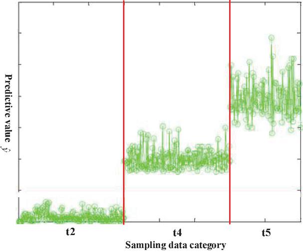
Figure 3 Text classification results based on WDAB-LSTM prototypical network.
In order to further analyze the performance of the WDAB-LSTM prototypical network, it is to be compared with the Siamese network [33] and prototypical network [34] with four indicators (accuracy rate, precision rate, recall rate, and F value) shown in Equations (8)–(11).
| (8) | |
| (9) | |
| (10) | |
| (11) |
where TP is the number of true positive classes; TN is the number of true negative classes; FP is the number of false positive classes; is the number of false negative classes.
The Siamese network is an architecture that includes two identical neural networks. The few-shot text classification method based on twin networks utilizes a convolutional neural network model with dual shared parameters to extract sample features, construct feature vectors, calculate the distance between vectors, and determine whether the samples belong to the same class based on the size of the distance. The prototypical network represents categories in the dataset as vectors and then the distance between these vectors and those of the new samples is calculated, where the nearest one decides which category the new samples should fall into. Compared with the Siamese network and prototypical network, the proposed algorithm can integrate shallow syntactic and high-level semantic information in sample sentences, resulting in richer and more effective information. The comparison of the four indicators for three algorithms is shown in Figures 4–7. The results show that each index of the WDAB-LSTM prototypical network is superior to the Siamese network and prototypical network, and the growth rate of each index is faster.
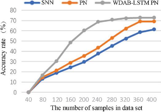
Figure 4 A comparison of accuracy rate of the three algorithms.
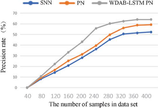
Figure 5 A comparison of precision rate of the three algorithms.
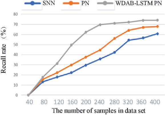
Figure 6 A comparison of recall rate of the three algorithms.
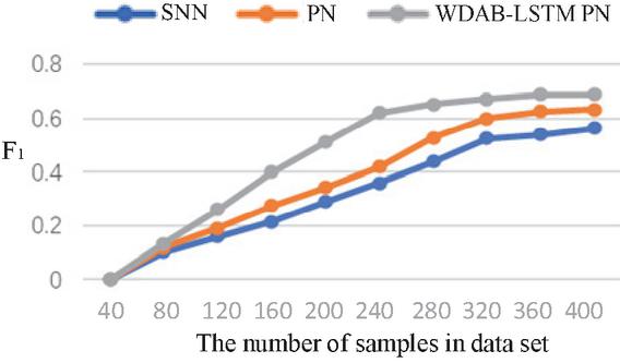
Figure 7 A comparison of the F value of the three algorithms.
For a fairer comparison, experiments are conducted 50 times with different test sets for average values of the four indicators. The experimental results are shown in Table 2.
Table 2 Comparison results of average indicators
| Average | Average | Average | Average | |
| Accuracy | Precision | Recall | ||
| Model | Rate (%) | Rate (%) | Rate (%) | Value |
| Siamese network | 60.25 | 51.63 | 60.83 | 0.558 |
| Prototypical network | 68.17 | 58.28 | 67.92 | 0.627 |
| WDAB-LSTM prototypical network | 72.35 | 62.79 | 72.29 | 0.672 |
To further test the performance of the proposed algorithm, compare the error rates of the proposed algorithm, Siamese network, and prototypical network based on TREC, and Kaggle datasets. Among them, TREC datasets from the Defense Advanced Research Projects Agency and the National Institute of Standards and Technology. Kaggle datasets from Google. During testing, the data is divided into short text and long text, with a maximum of 255 characters in short text. The test results are shown in Table 3. According to the test results, the error rate of the WDAB-LSTM prototypical network algorithm is lower for both short text classification and long text classification.
Table 3 Comparison results of errors rate
| Datasets Model | TREC | Kaggle | ||
| Short Text | Long Text | Short Text | Long Text | |
| Siamese network | 38.24% | 42.58% | 36.89% | 40.85% |
| Prototypical network | 31.76% | 35.52% | 30.23% | 35.07% |
| WDAB-LSTM prototypical network | 26.02% | 28.19% | 23.47% | 25. 38% |
It can be seen from Figures 4–7 and Tables 2 and 3 that the WDAB-LSTM prototypical network model proposed in this paper has a good effect on feature extraction and sample representation of few-shot text data and performs better both in single and repeated experiments when it is subjected to an evaluation of the four indicators (accuracy rate, precision rate, recall rate, and value). In addition, the error rates of text classification with the three algorithms were tested using the TREC and Kaggle datasets, and the proposed algorithm had the lowest error rate. The reason is that on the one hand text enhancement and text preprocessing expand the sample size of the dataset and on the other the optimized text features and distance measurement makes the outputs vectors contain important context-related information.
5 Conclusion
In this paper, the WDAB-LSTM prototypical network algorithm is proposed to solve the problems of insufficient feature representation and the insignificant effect of few-shot text classification. This algorithm optimizes the representation of text features to output vectors containing important context-related information so that the negative impact of improper selection of distance measurement module would be eliminated. In addition, through text enhancement and text preprocessing, this paper alleviates the problem of scarcity of few-shot text data resources. Simulation results show that with the proposed model the average accuracy rate increases by 12.1% and 4.18% respectively, compared with the Siamese network and the prototypical network, the average precision rate increased by 11.16% and 4.51%, the average recall rate by 11.64% and 4.37% and the value by 0.114 and 0.045; the average error rate reduced by 13.88% and 7.38%, which displays a better performance in feature representation and effective classification. Despite the improvement, future work needs to find better algorithms and network structures for measurement modules. The main problem is to avoid over-dependence on original data for similarity calculation.
Acknowledgments
This project is supported by the Major Projects of the National Social Science Foundation of China (18ZDA032).
References
[1] D. P. Wang, Z. W. Wang, L. L. Cheng, et al., “Few-Shot text classification with global-local feature information”, Sensors, vol. 22, no. 12, pp. 2022.
[2] W. F. Liu, J. M. Pang, N. Li, et al., “Few-shot short-text classification with language representations and centroid similarity”, Applied Intelligence, DOI: 10.1007/s10489-022-03880-y, 2022.
[3] Y. Wang, Q. Yao, J. T. Kwok, et al., “Generalizing from a few examples: A survey on fewshot learning”, ACM Computing Surveys, vol. 53, no. 3, pp. 1–34, 2020.
[4] A. Gupta, R. Bhatia, “Knowledge based deep inception model for web page classification”, Journal of Web Engineering, vol. 20, no. 7, pp. 2131–2167, 2021.
[5] J. Guan, R. Xu, J. Ya, et al., “Few-shot text classification with external knowledge expansion”, 5th International Conference on Innovation in Artificial Intelligence (ICIAI 2021, 2021, pp. 184–189.
[6] B. Hui, L. Liu, J. Chen, et al., “Few-shot relation classification by context attention-based prototypical networks with BERT”, Eurasip Journal on Wireless Communications and Networking, vol. 1, 2020.
[7] Y. Huang, L. Wang, “Acmm: Aligned cross-modal memory for few-shot image and sentence matching”, IEEE/CVF International Conference on Computer Vision, 2019, pp. 5773–5782.
[8] C. Z. Fu, C. R. Liu, C. T. Ishi, et al., “SeMemNN: A semantic matrix-based memory neural network for text classification”, IEEE 14th International Conference on Semantic Computing, 2020, pp. 123–127.
[9] L. M. Yan, Y. H. Zheng, J. Cao, “Few-shot learning for short text classification”, Multimedia Tools and Applications, vol. 77, no. 22, pp. 29799–29810, 2018.
[10] A. Santoro, S. Bartunov, M. Botvinick, et al., “One-shot learning with memory-augmented neural networks”, arXiv, 10.48550/arXiv.1605.06065, 2016.
[11] R. Geng, B. Li, Y. Li, et al., “Dynamic memory induction networks for few-shot text classification”, Proceedings of the 58th Annual Meeting of the Association for Computational Linguistics, 2020 pp. 1087–1094.
[12] Y. Lee, S. Choi, “Gradient-based meta-learning with learned layerwise metric and subspace”, Proceedings of the 35th International Conference on Machine Learning, 2018, pp. 2933–2942.
[13] A. Rajeswaran, C. Finn, S. M. Kakade, et al. “Meta-learning with implicit gradients”, Advances in Neural Information Processing Systems 32: Annual Conference on Neural Information Processing Systems, 2019, pp. 113–124.
[14] C. Finn, P. Abbeel, S. Levine, “Model-agnostic meta-learning for fast adap-tation of deep networks”, 10.48550/arXiv.1703.03400, 2017.
[15] T. Munkhdalai, H. Yu, “Meta networks”, International Conference on Machine Learning, 2017, pp. 2554–2563.
[16] M. Yu, X. Guo, J. Yi, et al., “Diverse fewshot text classification with multiple metrics”, arXiv:1805.07513, 2018.
[17] S. Ravi, A. Beatson, “Amortized bayesian meta-learning”, International Conference on Learning Representations, 2019.
[18] M. Qu, T. Gao, L. A. C. Xhonneux, et al., “Few-shot relation extraction via bayesian meta-learning on relation graphs”, Proceedings of the 37th Interna-tional Conference on Machine Learning, 2020, pp. 7867–7876.
[19] H. Lee, H. Lee, D. Na, et al., “Learning to balance: Bayesian meta-learning for imbalanced and out-of-distribution tasks”, 8th International Conference on Learning Representations, 2020.
[20] M. Hao, W. J. Wang, F. Zhou, “Joint representations of texts and labels with compositional loss for short text classification”, Journal of Web Engineering, vol. 20, no. 3, pp. 669–687, 2021.
[21] J. Yoon, T. Kim, O. Dia, et al., “Bayesian model-agnostic meta-learning”, Advances in Neural Information Processing Systems 31: Annual Conference on Neural Information Processing Systems, 2018, pp. 7343–7353.
[22] G. Koch, R. Zemel, R. Salakhutdinov, “Siamese neural networks for one-shot image recognition”, ICML Deep Learning Workshop, vol. 2, 2015.
[23] C. Zhang, Y. Cai, G. Lin, et al., “Deepemd: Few-shot image classification with differentiable earth mover’s distance and structured classifiers”, Proceedings of the IEEECVF Conference on Computer Vision and Pattern Recognition, 2020, pp. 12203–12213.
[24] F. Sung, Y. Yang, L. Zhang, et al., “Learning to compare: Relation network for few-shot learning”, Proceedings of the IEEE Conference on Computer Vision and Pattern Recognition, 2018, pp. 1199–1208.
[25] J. Snell, K. Swersky, et al., “Prototypical networks for few-shot learning”, Advances in Neural Information Processing Systems, pp. 4077–4087, 2017.
[26] A. Li, W. Huang, X. Lan, et al., “Boosting few-shot learning with adaptive margin loss”, 2020 IEEE/CVF Conference on Computer Vision and Pattern Recognition, 2020, pp. 12573–12581.
[27] J. Wei, K. Zou, “Eda: Easy data augmentation techniques for boosting performance on text classification tasks”, arXiv preprint arXiv:1901.11196, 2019.
[28] J. Pennington, R. Socher, C. D. Manning, “Glove: Global vectors for word representation”, Proceedings of the 2014 Conference on Empirical Methods in Natural Language Processing, 2014, pp. 1532–1543.
[29] L. H. Feng, L. B. Qiao, Y. Han, et al., “Syntactic enhanced projection network for few-shot chinese event extraction”, Lecture Notes in Artificial Intelligence, vol. 12816, pp. 75–87, 2021.
[30] Y. Xiao, Y. C. Jin, K. R. Hao, “Adaptive prototypical networks with label words and joint representation learning for few-shot relation classification”, IEEE Transactions on Neural Networks and Learning Systems, DOI: 10.1109/TNNLS.2021.3105377, 2021.
[31] A. Banerjee, X. Guo, H. Wang, “On the optimality of conditional expectation as a Bregman predictor”, IEEE Transactions on Information Theory, vol. 51, no. 7, pp. 2664–2669, 2005.
[32] X. Y. Gao, B. J. Tian, X. D. Tian, “Hesitant fuzzy graph neural network-based prototypical network for few-shot text classification”, Electronics, vol. 11, no. 15, pp. 2022.
[33] G. Koch, R. Zemel, R. Salakhutdinov, “Siamese neural networks for oneshot image recognition”, ICML Deep Learning Workshop, vol. 2, 2015.
[34] J. Snell, K. Swersky, R. S. Zemel, “Prototypical networks for fewshot learning”, arXiv preprint arXiv:1703.05175, 2017.
Biographies
Jing Peng received her bachelor’s and master’s degree in English language and literature respectively from Sichuan International Studies University in 2005 and Shanghai International Studies University in 2010. She is currently pursuing her Ph.D degree in logic in the School of Philosophy, Anhui University. Her current research interests include natural language processing, fuzzy logic and artificial intelligence logic.

Shuquan Huo received his bachelor’s degree in foreign philosophy from Zhengzhou University, his master’s degree in foreign philosophy from Sun Yat-sen University, and the philosophy of doctorate degree from Nankai University, respectively. He is currently working as a Professor at the Henan University. His research areas include modern logic, philosophy of language, and philosophy of mind.
Journal of Web Engineering, Vol. 22_3, 497–514.
doi: 10.13052/jwe1540-9589.2235
© 2023 River Publishers