Classification of Firewall Log Files with Different Algorithms and Performance Analysis of These Algorithms
Ebru Efeoğlu1 and Gurkan Tuna2,*
1Kutahya Dumlupinar University Software Department, Turkey
2Department of Computer Programming, Trakya University, Turkey
E-mail: gurkantuna@trakya.edu.tr
*Corresponding Author
Received 24 December 2022; Accepted 26 April 2024
Abstract
Classifying firewall log files allows analysing potential threats and deciding on appropriate rules to prevent them. Therefore, in this study, firewall log files are classified using different classification algorithms and the performance of the algorithms are evaluated using performance metrics. The dataset was prepared using the log files of a firewall. It was filtered to make it free from any personal data and consisted of 12 attributes in total and from these attributes the action attribute was selected as the class. In the performance evaluation, Simple Cart and NB tree algorithms made the best predictions, achieving an accuracy rate of 99.84%. Decision Stump had the worst prediction performance, achieving an accuracy rate of 79.68%. As the total number of instances belonging to each of the classes in the dataset was not equal, the Matthews correlation coefficient was also used as a performance metric in the evaluations. The Simple Cart, BF tree, FT tree, J48 and NB Tree algorithms achieved the highest average values. However, although the reset-both class was not predicted successfully by the others, the Simple Cart algorithm made the best predictions for it. The values of other performance metrics used in this study also support this conclusion. Therefore, the Simple Cart algorithm is recommended for use in classifying firewall log files. However, there is a need to develop a prefiltering and parsing approach to process different log files as each firewall brand creates and maintains log files in its own format. Therefore, in this study, a novel prefiltering and parsing approach has been proposed to process log files with different structures and create structured datasets using them.
Keywords: Firewalls, log files, classification, performance metrics, the Simple Cart algorithm.
1 Introduction
A firewall can control what traffic comes in and what traffic goes out. It monitors incoming and outgoing traffic, typically logs all traffic going through it and has some alerting capability. By inspecting the source and destination IP addresses and the destination port of all existing connections, it decides if the connections will be allowed or not. It is used for two main purposes: [1] protecting the network from threats from external and internal sources, [2] acting as an information resource for network experts and information security professionals’ tracking how a breach penetrated [1].
Firewalls are configured using rules. To be effective and successful, a reliable logging capability is essential for all firewalls. Because the logging capability of a firewall records how the firewall manages traffic types and allows seeing if new firewall rules work as expected and discovering malicious activities within the network if there are [2]. Information provided by firewall logs assists in investigating a cyber attack and creates rules to stop connections from specific IP addresses [1]. The firewall logs can be seen as the first layer of tracking hackers’ moves. Reviewing the firewall logs allows determining what the hackers are looking for.
Monitoring and periodic evaluation of firewall log files plays a key role in achieving the desired level of information security. By analysing firewall log files, network administrators can identify potential threats to their networks and then decide rules to prevent those threats [3]. Although security information and event management systems allow collecting logs from various network devices and servers and offer easy viewing and reporting solutions [4], they do not have the ability to analyse existing logs and classifying a new instance based on a set of attributes and the existing dataset.
Although classification of firewall log files was performed using different algorithms and the algorithms’ performances were compared based on well-known performance metrics, most of these studies, such as [3] and [5], focused on one or a few algorithms and a limited number of performance metrics were used in those studies. Different from the literature, in this study firewall log files were classified using different types of classification algorithms and the performances of the algorithms were evaluated using an extensive set of performance metrics. Moreover, as the number of instances belonging to each of the classes in the dataset used was not equal, in parallel with the conclusions in [6], the Matthews correlation coefficient was also used as a metric in the performance evaluation. The remainder of this paper is structured as follows. Section 2 presents a focused literature review. In Section 3, information about the dataset and classification algorithms used in this study is given. Performance analysis methodology and metrics used in this study are presented in Section 4. In Section 5, the results obtained in the performance evaluation study are reported and a discussion on the results is given. Section 6 concludes this paper.
2 Related Work
Monitoring and periodic evaluation of firewall log files is critically important for organisations in terms of data security. As firewall log analysis can be handled from different aspects of information security, researchers have used different methodologies for it. In [7] a framework was introduced to explore and learn representations of log data created by firewalls with the purpose of identifying advanced persistent threats. The framework in [7] relies on a divide-and-conquer approach that combines behavioural analytics, time series modelling and representation learning algorithms so that large volumes of data can be modelled. It was demonstrated that the use of the presented approach on a given dataset extracted from 3 billion log lines achieved an area under the receiver operating characteristic (ROC) curve of 0.943 on the test dataset.
Most anomaly detection based systems rely on monitoring traffics or searching logs and do not focus on analysing attack processes [8]. However, advanced cyber attacks are often characterised by multiple types, different layers, and a number of stages [8]. Therefore, complex multistage attacks cannot be fully modelled. With the goal of addressing this issue in [8] a multistage intrusion analysis system was proposed. The proposed system integrates traffic with logs of network devices through data association rules and allows correlating log data with traffic characteristics. This way it fully reflects the attack process and helps to build a federated detection system. Therefore, the proposed system can discover the steps of cyber attacks with high accuracy and few false positives, as well as providing information about the current network status and the behaviours of normal users [8].
By filtering out all incoming packets and in some cases outgoing packets as well, a firewall protects computer networks and this is carried out by matching the packets against a set of rules [5]. The firewall either allows or denies, or drops/resets the incoming packets by relying on an automated classification process. In [5], a novel classification model was proposed to determine an appropriate action for each packet by analysing packet attributes. The proposed model is based on a shallow neural network (SNN) with 150 neurons in the hidden layer to train and then classify the dataset into three classes as allow, deny, and drop/reset. After 381 epochs, the proposed model achieved an overall accuracy of 98.5%.
As the analysis of firewall logs plays a key role in achieving the desired level of information security, in [3] the use of a multiclass support vector machine (SVM) to classify firewall logs was presented. The log file used in [3] was obtained from a Palo Alto 5020 firewall used at a state university in Türkiye. Linear, polynomial, sigmoid and radial basis functions were used as the activation function for the SVM [3]. The log file consisting of 65,532 instances was examined using 11 features [3]. The action attribute was selected as the class and allow, deny, drop and reset-both parameters were implemented for it. It was shown that a recall value of 0.985 was achieved when the SVM was used with the sigmoid activation function and a precision value of 0.675 was achieved when the SVM was used with the linear activation function. On the other hand, when the SVM was used with the radial basis function, the highest F1 score value of 0.764 was achieved. If all the performance metrics were taken into consideration, the radial basis function was the best activation function for firewall log classification using the SVM.
Firewall security policies are created and implemented using rules. However, an anomaly in firewall rules can create serious security risks. In addition, a manual check of the firewall rules is not efficient and may sometimes not be sufficient to detect existing anomalies [9]. Therefore, in [9], an automated model was proposed to detect anomalies in firewall logs. In the proposed model, firewall logs are first analysed to extracted features. Then the extracted features are processed by different classification algorithms, namely naive Bayes (NB), K-nearest neighbours (KNN), decision table and HyperPipes. As the results obtained in the performance evaluation demonstrated, the KNN achieved the best results. Then, a model was proposed using the F-measure distribution. Using this model, 93 firewall rules were analysed and it was shown that the model successfully anticipated six firewall rules that caused anomaly.
Although in recent years cyber attacks have been a serious and growing concern for organisations and individuals, the process of analysing log files using traditional methods is unorganised and inefficient. Moreover, when it is done manually, firewall log analysis takes a significant time to investigate [10]. Therefore, in [10] a novel approach was proposed to help analysts identify cyber events. The proposed approach helps to analyse log files more efficiently; this way potential anomalies can be discovered more easily [10]. The approach called tabulated vector approach creates meaningful state vectors from time-oriented blocks. Then, in a human–machine collaborative interface, state vectors are analysed using multivariate and graphical analysis. Outlier detection can be done using statistical tools, such as the histogram matrices, factor analysis, and Mahalanobis distance [10].
3 Dataset and Classification Algorithms
In this study, the dataset used in [3] was used. The instances in the dataset were the actual log records of a Palo Alto 5020 firewall. As stated in [3], before processing all personal data was removed from the actual logs. The dataset consists of 65,428 records. Table 1 represents information about the dataset. As listed in Table 1, there are 12 features (attributes) in total and from these attributes action attribute was selected as the class. Allow, deny, drop and reset-both parameters were implemented for the action class.
In this study, an extensive set of classification algorithms was used to identify the class of a new instance (an incoming packet). The classification algorithms are explained as follows.
• Naïve Bayes: In this algorithm, the probability of finding the right class of an instance from a test dataset is calculated by multiplying the probabilities of all the factors affecting that result [11]. Based on these calculations, the class of the instance is determined [11].
• Sequential minimal optimisation (SMO): This can quickly solve the SVM and quadratic programming (KP) problem without using extra matrix space and numerical KP optimisation steps [12]. The SMO basically decomposes all KP problems into subproblems by means of the Osuna theorem, keeping convergence, and chooses to solve the smallest optimisation problem at each step [12]. As the Lagrangian multipliers must obey the linear equation rules, the smallest optimisation problem for the standard SVM KP problem includes two Lagrangian multipliers [12]. Then, at each step, The SMO optimises the two Lagrange multipliers together to find the best value for these multipliers and updates the SVM to reflect the new best values [12].
Table 1 Attributes and their descriptions
| Attribute | Attribute Description | Type | Min | Max | Mean |
| Source port | Client source port | Numerical | 0 | 65534 | 49387 |
| Destination port | Client destination port | Numerical | 0 | 65535 | 10592 |
| Nat source port | Network address translation source port | Numerical | 0 | 3850148 | 1862 |
| Nat destination port | Network address translation destination port | Numerical | 0 | 65535 | 2673 |
| Bytes | Total Bytes | Numerical | 0 | 9932735 | 25770 |
| Bytes sent | Bytes sent | Numerical | 0 | 3850148 | 1862 |
| Bytes received | Bytes received | Numerical | 0 | 9847344 | 23907 |
| Packets | Total packets | Numerical | 0 | 50585 | 33 |
| Elapsed time (s) | Elapsed time for flow | Numerical | 0 | 10824 | 65 |
| pkts_sent | Packets sent | Numerical | 0 | 24913 | 12 |
| pkts_received | Packets received | Numerical | 0 | 25672 | 20 |
| Action | Class (allow, deny, drop, reset-both) Allow: In the case of this class, the data traffic is allowed Deny: In the case of this class, the data traffic is blocked and the default deny action defined for the application is enforced. Drop: In the case of this class, the data traffic is silently dropped. A TCP reset is not sent to the device or application. Reset-both: In the case of this class, a TCP reset is sent to both the client-side and server-side devices. |
Nominal |
• KNN: This aims to classify instances based on the closest training instances in the feature space. The instance to be classified by the KNN is processed one by one with each instance in the training dataset [13]. In order to determine the class of the instance to be classified, k instances closest to the relevant instance in the training set are selected. Whichever class has the most instances in the set of selected instances, the tested instance belongs to this class. The distances between instances can be determined by different distance measures, and the Euclidean distance is often preferred [13].
• K*: This is based on the comparison of an unknown instance in the test dataset with the instances in the training dataset that were previously classified but not revealed in the database [14].
• Rep Tree: First proposed by Quinlan, it relies on regression tree logic [15]. With this logic, many trees are created in different iterations and then the best tree is selected among these decision trees. As a result, Rep Tree is based on the principle of minimising the error due to variance and information gain with entropy [16].
• Random tree: This is a supervised classifier that relies on many individual learners. Based on a bagging idea, it produces a random set of data to create a decision tree [17].
• Random forest: This is especially preferred because of its good performance in classifying large amounts of data. Instead of producing a single decision tree, it combines multiple decision trees, each of which is trained using different training datasets [18].
• Simple Cart: In this algorithm, decision trees are created by splitting each decision node into two different branches using various separation criteria [19].
• Extra trees: This is a collective learning technique that combines the results of multiple decision trees. Each decision tree is created from the original training dataset. The features are randomly sampled at each split point of a decision tree. Different from random forests, a split point is selected at random [20].
• Hoeffding tree: This relies on a statistical value, called the Hoeffding limit, at each node of the decision tree to make the decision about how to split the node. Each sample is read at most once and processed in an appropriate time interval [21].
• Decision Stump: This is a one level decision tree and uses the values of a single input feature for prediction [22]. It is applied to ensemble algorithms such as Adaboost [22].
• J48: This is based on C4.5 and ID3 algorithms. It works on nodes and child rows from child rows, with the logic of using one node from each tree [23]. In this context, it is widely accepted as one of the fastest and highest precision classification algorithms [23].
• FT tree: This uses the information of all input properties in both intermediate nodes and leaves [24]. A separate regression function is used at each decision node of the tree. With this function, the number of features is increased and which path to continue in the tree according to the obtained probabilities is decided. If a leaf is reached, that sample is either classified as a constant or arrives at another regression function in the leaf [24].
• Best-first decision tree (BF tree): This uses divide-and-conquer logic like standard tree algorithms. The best split node is added to the tree at each step. The best node is the one that maximises impurity among all nodes available for splitting. The best initial decision tree contains many features and the root nodes are placed according to these features [25].
• NB tree: This is a decision tree algorithm with NB classifiers in its leaves. Different from classical recursive partitioning schemes, in NB Tree, the generated leaf nodes are NB categorisers rather than nodes that predict a single class. As in decision trees, a threshold is selected for the features using the entropy technique [26].
• Radial basis function (RBF): This implements fully controlled radial basis function networks with the optimisation method, minimising the quadratic error. Classification and regression problems are considered together. In both cases, the squared error penalised by a quadratic penalty on unbiased weights in the output layer is employed as the loss function to obtain the network parameters [27].
• LADTree: The alternating decision tree (ADTree) combines decision trees with the predictive accuracy of boosting into a set of interpretable classification rules [28]. The logistic boosting (LogitBoost) algorithm [29] was fused with the induction of ADTrees. The LADTree learning algorithm relies on the LogitBoost algorithm so that an ADTree can be induced.
4 Performance Analysis and Metrics
In this study, K-fold cross-validation was preferred. The reason for preferring this technique is that in the case of an overfitting problem, while the model gives good results on the dataset studied, it makes unsuccessful predictions on the datasets, which has never been seen. The K-fold cross-validation technique has a single parameter called k, the number of groups that a given data sample is to be split into. The number of k is usually 10, as in this study. For each unique group, the group is either taken as a hold out or test dataset and then the remaining groups are taken as a training dataset. Firstly, a model is fit on the training dataset and then evaluated on the test dataset. Second, the evaluation score is retained and the model is discarded. Finally, the evaluation scores achieved in each round is summed up. This way the performance of the model is assessed.
Various criteria exist to evaluate how well a classification algorithm performs at the classification process. The most commonly used of these criteria is the confusion matrix, which consists of information about actual and predicted classes. The confusion matrix allows us to understand what class the samples are actually in and what class the algorithm predicts that sample as. The confusion matrix structure used in this study is given in Figure 1.
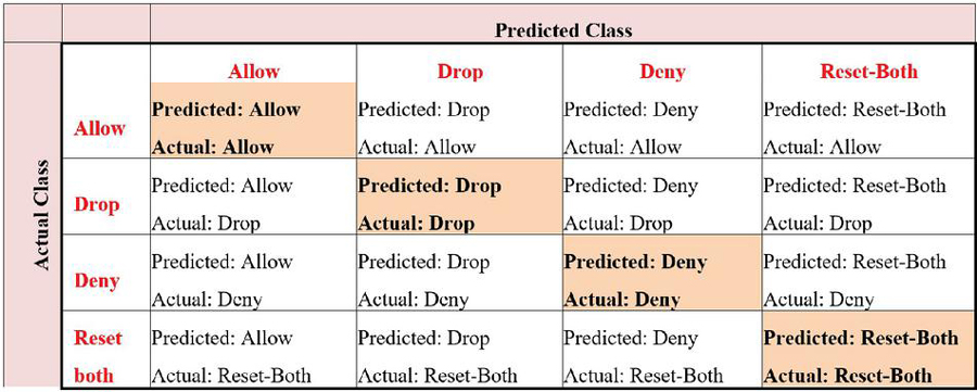
Figure 1 Confusion matrix of the firewall log classification.
As a result of a classification, four different situations arise as true positive (TP), true negative (TN), false positive (FP) and false negative (FN). FP and FN values occur when the predicted class is not the same as the actual class. These represent the number of instances that the algorithm predicted incorrectly. TP and TN values represent the values that the algorithm predicts correctly. Using these four values, some metrics for performance evaluation can be calculated. The metrics calculated using these values and their equations are presented in Table 2.
Table 2 Performance metrics and their formulas
| Metric | Equation |
| Accuracy | |
| TP rate (TPR) | |
| FP rate (FPR) | |
| Precision | |
| Recall | |
| F-measure | |
| Matthews correlation | |
| coefficient (MCC) |
Apart from the metrics specified in the table, there are other metrics that can be used in performance analysis. The analysis of ROC and precision-recall (PR) curves is important for performance evaluation. In a ROC curve, while the X axis shows FPR, the Y axis shows TPR. On the other hand, in a PR curve, the X axis is precision and the Y axis is the recall value. Therefore, the performance of a classification algorithm can be commented on by looking at the area value under these curves. The closer these values are to 1, the better the algorithm performed.
Kappa statistical value is another widely used metric. It measures the agreement between the actual classification and the classification made and has a value between 1 and 1. While a value of 1 is the indication of a complete mismatch, the value of 1 is the indication of a perfect fit. If the probabilistic accuracy of the classification algorithm P(x) is represented by the weighted average of the classification probability in the same dataset, P(y), the Kappa value can be calculated using (1).
| (1) |
The root mean square (RMS) error value is a criterion that shows how much error the classification is made. A low error rate in classification means that the classification is successful. It is calculated using (2).
| (2) |
where, is the estimated value and is the objective value.
5 Results, Discussion, and a Novel Log Prefiltering and Parsing Approach
The confusion matrices of all the algorithms used in this study are given in Figures 2 and 3. The values coloured in green represent the number of instances that the algorithms correctly classified.
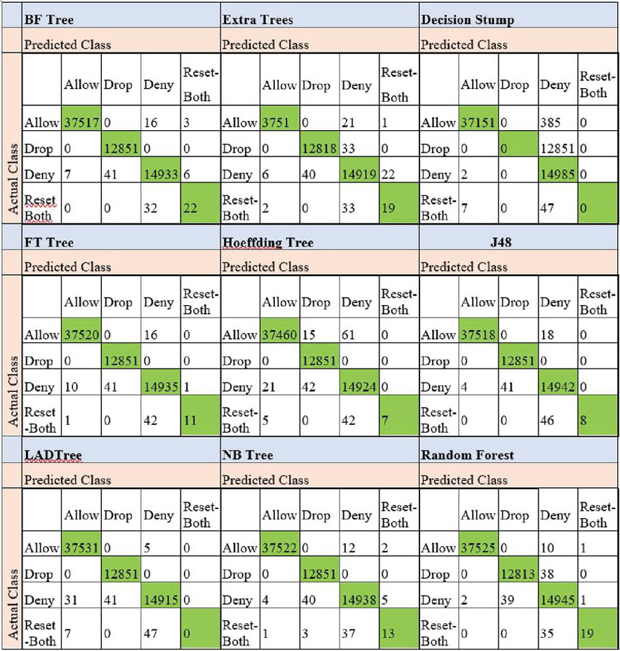
Figure 2 Confusion matrices of the firewall log classification when different classification algorithms were preferred.
An example of how to interpret this figure is as follows. As can be seen in Figure 2, the BF tree incorrectly classified 16 of the allow class instances as the drop class and 3 of the allow class instances as the reset-both class. However, it correctly classified all the instances belonging to the drop class. It incorrectly classified 7 of the deny class instances as the allow class and 41 of the deny class instances as the drop class. Moreover, it incorrectly classified 6 of the deny class instances as the reset-both class. Finally, the BF tree incorrectly classified 32 of the reset-both class instances as the deny class.
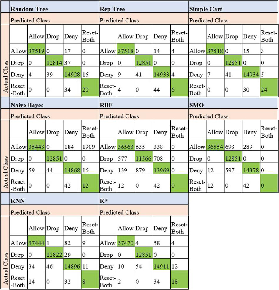
Figure 3 Confusion matrices of the firewall log classification when different classification algorithms were preferred.
The number of incorrectly classified instances belonging to each class (allow, drop, deny, reset-both) by each of the algorithms are listed in Table 3. As listed in Table 3, the least number of incorrectly predicted instances belongs to the drop class. On the other hand, as the total number of instances belonging to the classes in the dataset was not equal as shown in Figure 4, the low number of incorrect predictions for the reset-both class may be misleading. This is because the total number of data belonging to the reset-both class was less than the total number of instances belonging to the other classes. For this reason, considering just the number of incorrectly predicted instances or correctly predicted instances in order to make an accurate performance analysis may lead to misleading results.
Table 3 The total number of incorrectly classified instances
| The total number of incorrectly classified instances | |||||
| Algorithm | Allow | Drop | Deny | Reset-both | Total |
| BF tree | 19 | 0 | 47 | 32 | 198 |
| Extra trees | 22 | 33 | 68 | 35 | 158 |
| Decision Stump | 385 | 12851 | 2 | 54 | 13292 |
| FT tree | 16 | 0 | 52 | 43 | 111 |
| Hoeffding tree | 76 | 0 | 63 | 47 | 186 |
| J48 | 18 | 0 | 45 | 46 | 109 |
| LADTree | 5 | 0 | 72 | 54 | 131 |
| NB tree | 14 | 0 | 49 | 41 | 104 |
| Random forest | 11 | 38 | 42 | 35 | 126 |
| Random tree | 17 | 37 | 59 | 34 | 147 |
| Rep tree | 18 | 0 | 54 | 48 | 120 |
| Simple Cart | 18 | 0 | 53 | 30 | 101 |
| Naive Bayes | 2093 | 0 | 119 | 42 | 2254 |
| RBF | 973 | 1285 | 1018 | 54 | 3330 |
| SMO | 982 | 0 | 609 | 54 | 1645 |
| KNN | 92 | 29 | 91 | 46 | 258 |
| K* | 66 | 0 | 76 | 36 | 178 |
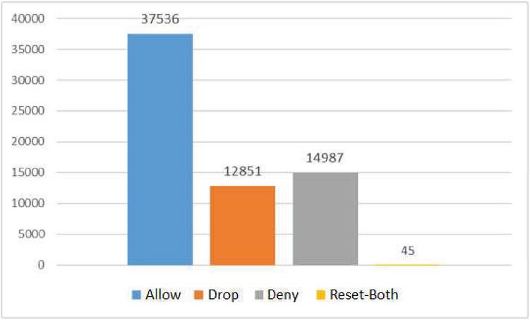
Figure 4 The total number of instances belonging to each class.
The accuracy rates of the algorithms are shown in Figure 5. As can be seen in Figure 5, the decision stump algorithm achieved the lowest accuracy rate. The highest accuracy rate obtained in the classifications was 99.84% and it was achieved by the Simple Cart and NB tree algorithms. However, evaluating the algorithms by just considering the accuracy rates is not reliable [30]. As the total number of data rows for each class was not equal in the dataset, i.e. imbalanced dataset, other performance metrics were also considered.
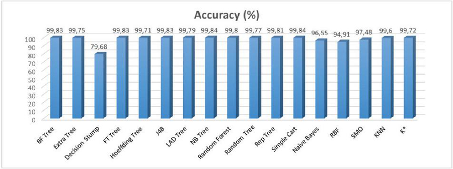
Figure 5 The accuracy rates of the classification algorithms.
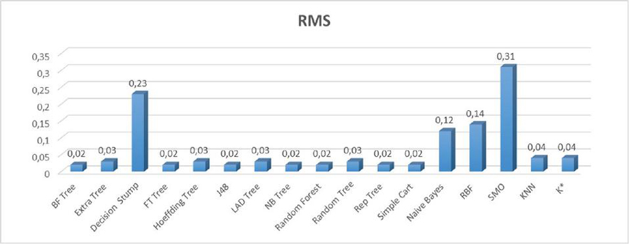
Figure 6 The RMS error values of the results obtained when different classification algorithms were preferred.
The RMS error values of all the algorithms are given in Figure 6. While the SMO algorithm had the highest RMS error value, the BF tree, the FT tree, the J48, the NB tree, the random forest, the rep tree and the Simple Cart algorithms had lower error rates compared to the remaining ones. In order to examine the performances of the algorithms in detecting each class (allow, drop, deny, reset-both), the other performance metrics were also calculated and they are presented in Table 4.
The remaining performance metrics of the classification algorithms are given in Table 4. While the Kappa statistical value of these metrics varied between 0.99 and 0.64, on average it was around 0.99. The lowest Kappa value obtained in this study was 0.64 and it belongs to the Decision Stump algorithm. When the other performance metrics are considered, it can be seen that the TPR varied between 0 and 0.99. As a TPR of zero indicates that the algorithm has not made any correct predictions, it is understood that the Decision Stump algorithm did not correctly predict the instances belonging to both the drop and the reset classes. Similarly, as the TPRs of the LADTree, the RBF and the SMO algorithms for the reset-both class are 0, it is understood that these algorithms incorrectly classified all the instances belonging to the reset-both class. However, it can be seen when the TPRs were considered; the BF tree, the FT tree, the Hoeffding tree, the J48, the LADTree, the NB tree, the rep tree, the Simple Cart and the NB algorithms correctly classified all the instances belonging to the drop class. Precision metric is an indicator of how many of the values predicted as positive by the algorithm are actually positive. Although a precision value of 1 was obtained in the classification, some of the algorithms achieved very low precision value for the reset-both class, even the precision value could not be calculated for the Decision Stump, the LADTree, the RBF and the SMO algorithms.
Table 4 Performance metrics for each classification algorithm
| BF tree | |||||||||
| Class | TPR | FPR | Precision | Recall | F-measure | MCC | ROC Area | PRC Area | Kappa |
| Allow | 0.999 | 0.0 | 1 | 0.999 | 1 | 0.999 | 1 | 1 | 0.997 |
| Drop | 1 | 0.001 | 0.997 | 1 | 0.998 | 0.998 | 1 | 0.996 | |
| Deny | 0.996 | 0.001 | 0.997 | 0.996 | 0.997 | 0.996 | 0.999 | 0.997 | |
| Reset-both | 0.407 | 0 | 0.710 | 0.407 | 0.518 | 0.537 | 0.888 | 0.350 | |
| Average | 0.998 | 0.001 | 0.998 | 0.998 | 0.998 | 0.998 | 0.999 | 0.998 | |
| Extra trees | |||||||||
| Class | TPR | FPR | Precision | Recall | F-measure | MCC | ROC Area | PRC Area | Kappa |
| Allow | 0.999 | 0 | 1 | 0.999 | 1 | 0.999 | 1 | 1 | 0.995 |
| Drop | 0.997 | 0.001 | 0.997 | 0.997 | 0.997 | 0.996 | 0.998 | 0.995 | |
| Deny | 0.995 | 0.002 | 0.994 | 0.995 | 0.995 | 0.993 | 0.997 | 0.991 | |
| Reset-both | 0.352 | 0 | 0.452 | 0.352 | 0.396 | 0.399 | 0.676 | 0.160 | |
| Average | 0.998 | 0.001 | 0.997 | 0.998 | 0.998 | 0.997 | 0.999 | 0.996 | |
| Decision Stump | |||||||||
| Class | TPR | FPR | Precision | Recall | F-measure | MCC | ROC Area | PRC Area | Kappa |
| Allow | 0.990 | 0 | 1 | 0.990 | 0.995 | 0.988 | 0,994 | 0.997 | 0.646 |
| Drop | 0 | 0 | – | 0 | — | — | 0.853 | 0.454 | |
| Deny | 1 | 0.263 | 0.530 | 1 | 0.693 | 0.625 | 0.868 | 0.529 | |
| Reset-both | 0 | 0 | — | 0 | – | — | 0.689 | 0.001 | |
| Average | 0.797 | 0.061 | — | 0.797 | – | —- | 0.937 | 0.782 | |
| FT tree | |||||||||
| Class | TPR | FPR | Precision | Recall | F-measure | MCC | ROC Area | PRC Area | Kappa |
| Allow | 1 | 0 | 1 | 1 | 1 | 0.999 | 1 | 1 | 0.997 |
| Drop | 1 | 0.001 | 0.997 | 1 | 0.998 | 0.998 | 1 | 0.995 | |
| Deny | 0.997 | 0.001 | 0.996 | 0.997 | 0.996 | 0.995 | 0.999 | 0.997 | |
| Reset-both | 0.204 | 0 | 0.917 | 0.204 | 0.333 | 0.432 | 0.932 | 0.182 | |
| Average | 0.998 | 0.001 | 0.998 | 0.998 | 0.998 | 0.998 | 1 | 0.998 | |
| Hoeffding tree | |||||||||
| Class | TPR | FPR | Precision | Recall | F-measure | MCC | ROC Area | PRC Area | Kappa |
| Allow | 0.998 | 0.001 | 0.999 | 0.998 | 0.999 | 0.997 | 0.999 | 0.999 | 0.995 |
| Drop | 1 | 0.001 | 0.996 | 1 | 0.998 | 0.997 | 1 | 0.996 | |
| Deny | 0.996 | 0.002 | 0.993 | 0.996 | 0.994 | 0.993 | 0.998 | 0.993 | |
| Reset-both | 0.130 | 0 | 1 | 0.130 | 0.230 | 0.360 | 0.839 | 0.153 | |
| Average | 0.997 | 0.001 | 0.997 | 0.997 | 0.997 | 0.995 | 0.999 | 0.996 | |
| J48 | |||||||||
| Class | TPR | FPR | Precision | Recall | F-measure | MCC | ROC Area | PRC Area | Kappa |
| Allow | 1 | 0 | 1 | 1 | 1 | 0.999 | 1 | 1 | 0.997 |
| Drop | 1 | 0.001 | 0.997 | 1 | 0.998 | 0.998 | 1 | 0.996 | |
| Deny | 0.997 | 0.001 | 0.996 | 0.997 | 0.996 | 0.995 | 0.999 | 0.996 | |
| Reset-both | 0.148 | 0 | 1 | 0.148 | 0.258 | 0.385 | 0.924 | 0.158 | |
| Average | 0.998 | 0.001 | 0.998 | 0.998 | 0.998 | 0.998 | 1 | 0.998 | |
| LADTree | |||||||||
| Class | TPR | FPR | Precision | Recall | F-measure | MCC | ROC Area | PRC Area | Kappa |
| Allow | 1 | 0.001 | 0.999 | 1 | 0.999 | 0.999 | 1 | 1 | 0.996 |
| Drop | 1 | 0.001 | 0.997 | 1 | 0.998 | 0.998 | 1 | 0.996 | |
| Deny | 0.995 | 0.001 | 0.997 | 0.995 | 0.996 | 0.995 | 0.999 | 0.997 | |
| Reset-both | 0 | 0 | — | 0 | — | — | 0.933 | 0.104 | |
| Average | 0.998 | 0.001 | — | 0.998 | — | — | 1 | 0.998 | |
| NB tree | |||||||||
| Class | TPR | FPR | Precision | Recall | F-measure | MCC | ROC Area | PRC Area | Kappa |
| Allow | 1 | 0 | 1 | 1 | 1 | 0.999 | 1 | 1 | 0.997 |
| Drop | 1 | 0.001 | 0.997 | 1 | 0.998 | 0.998 | 1 | 0.997 | |
| Deny | 0.997 | 0.001 | 0.997 | 0.997 | 0.997 | 0.996 | 0.999 | 0.998 | |
| Reset-both | 0.241 | 0 | 0.650 | 0.241 | 0.351 | 0.395 | 0.942 | 0.241 | |
| Average | 0.998 | 0 | 0.998 | 0.998 | 0.998 | 0.998 | 1 | 0.998 | |
| Random tree | |||||||||
| Class | TPR | FPR | Precision | Recall | F-measure | MCC | ROC Area | PRC Area | Kappa |
| Allow | 1 | 0 | 1 | 1 | 1 | 0.999 | 1 | 1 | 0.996 |
| Drop | 0.997 | 0.001 | 0.997 | 0.997 | 0.997 | 0.996 | 0.998 | 0.995 | |
| Deny | 0.996 | 0.002 | 0.994 | 0.996 | 0.995 | 0.994 | 0.997 | 0.992 | |
| Reset-both | 0.370 | 0 | 0.556 | 0.370 | 0.444 | 0.453 | 0.685 | 0.206 | |
| Average | 0.998 | 0.001 | 0.998 | 0.998 | 0.998 | 0.997 | 0.999 | 0.996 | |
| Rep tree | |||||||||
| Class | TPR | FPR | Precision | Recall | F-measure | MCC | ROC Area | PRC Area | Kappa |
| Allow | 1 | 0 | 1 | 1 | 1 | 0.999 | 1 | 1 | 0.996 |
| Drop | 1 | 0.001 | 0.997 | 1 | 0.998 | 0.998 | 1 | 0.996 | |
| Deny | 0.996 | 0.001 | 0.996 | 0.996 | 0.996 | 0.995 | 0.999 | 0.997 | |
| Reset-both | 0.111 | 0 | 0.429 | 0.111 | 0.176 | 0.218 | 0.905 | 0.100 | |
| Average | 0.998 | 0.001 | 0.998 | 0.998 | 0.998 | 0.997 | 1 | 0.998 | |
| Simple Cart | |||||||||
| Class | TPR | FPR | Precision | Recall | F-measure | MCC | ROC Area | PRC Area | Kappa |
| Allow | 1 | 0 | 1 | 1 | 1 | 0.999 | 1 | 1 | 0.997 |
| Drop | 1 | 0.001 | 0.997 | 1 | 0.998 | 0.998 | 1 | 0.996 | |
| Deny | 0.996 | 0.001 | 0.997 | 0.996 | 0.997 | 0.996 | 0.999 | 0.997 | |
| Reset-both | 0.444 | 0 | 0.750 | 0.444 | 0.558 | 0.577 | 0.966 | 0.408 | |
| Average | 0.998 | 0.001 | 0.998 | 0.998 | 0.998 | 0.998 | 1 | 0.998 | |
| Naive Bayes | |||||||||
| Class | TPR | FPR | Precision | Recall | F-measure | MCC | ROC Area | PRC Area | Kappa |
| Allow | 0.944 | 0.002 | 0.998 | 0.944 | 0.971 | 0.935 | 0.998 | 0.998 | 0.942 |
| Drop | 1 | 0.001 | 0.997 | 1 | 0.998 | 0.998 | 1 | 0.997 | |
| Deny | 0.992 | 0.004 | 0.985 | 0.992 | 0.989 | 0.985 | 0.998 | 0.995 | |
| Reset-both | 0.222 | 0.029 | 0.006 | 0.222 | 0.012 | 0.033 | 0.912 | 0.043 | |
| Average | 0.966 | 0.002 | 0.994 | 0.966 | 0.979 | 0.958 | 0.998 | 0.996 | |
| RBF | |||||||||
| Class | TPR | FPR | Precision | Recall | F-measure | MCC | ROC Area | PRC Area | Kappa |
| Allow | 0.974 | 0.026 | 0.980 | 0.974 | 0.977 | 0.947 | 0.995 | 0.997 | 0.912 |
| Drop | 0.900 | 0.029 | 0.884 | 0.900 | 0.892 | 0.865 | 0.977 | 0.911 | |
| Deny | 0.932 | 0.022 | 0.928 | 0.932 | 0.930 | 0.909 | 0.992 | 0.976 | |
| Reset-both | 0 | 0 | — | 0 | — | — | 0.492 | 0.002 | |
| Average | 0.949 | 0.026 | —- | 0.949 | —- | — | 0.990 | 0.974 | |
| SMO | |||||||||
| Class | TPR | FPR | Precision | Recall | F-measure | MCC | ROC Area | PRC Area | Kappa |
| Allow | 0.974 | 0.001 | 0.999 | 0.974 | 0.986 | 0.959 | 0.989 | 0.991 | 0.957 |
| Drop | 1 | 0.025 | 0.909 | 1 | 0.952 | 0.942 | 0.988 | 0.909 | |
| Deny | 0.959 | 0.007 | 0.977 | 0.959 | 0.968 | 0.959 | 0.981 | 0.949 | |
| Reset-both | 0 | 0 | — | 0 | — | — | 0.682 | 0.001 | |
| Average | 0.975 | 0.007 | — | 0.975 | — | — | 0.987 | 0.965 | |
| KNN | |||||||||
| Class | TPR | FPR | Precision | Recall | F-measure | MCC | ROC Area | PRC Area | Kappa |
| Allow | 0.998 | 0.002 | 0.999 | 0.998 | 0.998 | 0.996 | 0.998 | 0.998 | 0.993 |
| Drop | 0.998 | 0.001 | 0.996 | 0.998 | 0.997 | 0.996 | 0.999 | 0.994 | |
| Deny | 0.994 | 0.003 | 0.990 | 0.994 | 0.992 | 0.990 | 0.996 | 0.989 | |
| Reset-both | 0.148 | 0 | 0.286 | 0.148 | 0.195 | 0.205 | 0.515 | 0.040 | |
| Average | 0.996 | 0.002 | 0.996 | 0.996 | 0.996 | 0.994 | 0.997 | 0.994 | |
| K* | |||||||||
| Class | TPR | FPR | Precision | Recall | F-measure | MCC | ROC Area | PRC Area | Kappa |
| Allow | 0.998 | 0 | 1 | 0.998 | 0.999 | 0.998 | 1 | 1 | 0.995 |
| Drop | 1 | 0.001 | 0.996 | 1 | 0.998 | 0.997 | 0.999 | 0.995 | |
| Deny | 0.995 | 0.002 | 0.994 | 0.995 | 0.994 | 0.993 | 0.999 | 0.996 | |
| Reset-both | 0.333 | 0 | 0.529 | 0.333 | 0.409 | 0.420 | 0.955 | 0.314 | |
| Average | 0.997 | 0.001 | 0.997 | 0.997 | 0.997 | 0.996 | 0.999 | 0.998 | |
In general, precision is especially important when the FPR is high. When the proposed use of the classification algorithms is considered for real-time implementations, if some instances are incorrectly predicted as the deny class, the information/messages associated with those instances will be denied or dropped and this may lead to information loss. Therefore, a high precision value is an important criterion in choosing the best classification algorithm for the proposed use. On the other hand, when an instance actually belongs to one of the deny, drop or reset-both classes, it must be correctly predicted. Otherwise it can lead to a significant security risk. In such case, silently dropping the packet is always the best choice.
Recall shows how successfully positive instances are predicted varies between 1 and 0. As the highest recall values of the algorithms were obtained for the drop class, all the classification algorithms are more successful in classifying the instances belonging to the drop class than the ones belonging to the other classes.
F-measure is the harmonic average of precision and recall and is preferred in case of incompatible recall and precision values, such as low recall and high recall or vice versa. Considering the average F-measure values of all the classification algorithms, it can be seen that the NB algorithm had the lowest F-measure value of 0.979. While the F-measure values of the other algorithms were 0, 0.998, 0.997 and 0.996, the F-measure values of the Decision Stump, the LADTree, the RBF, and the SMO algorithms could not be calculated. The reason why the average F-measure values of the LADTree, the RBF, and the SMO algorithms could not be calculated is because the precision value could not be calculated for the reset-both class. Likewise, the average F-measure value of the Decision Stump algorithm could not be calculated, as the precision value could not be calculated for the drop and reset-both classes.
Considering the MCC value, which is generally preferred to evaluate the classification performance when unbalanced datasets are used, the BF tree, the FT tree, the J48, the NB tree and the Simple Cart algorithms achieved the highest average MCC values.
Overall, the ROC area values of the allow and drop classes of all the classification algorithms are higher than the other classes. When the FT tree, the J48, the LADTree, the NB tree, the rep tree, and the Simple Cart algorithms were used, the average ROC area value was 1. The average PRC area value varied between 0.782 and 1 and the Decision Stump algorithm had the lowest one for this metric. In parallel with the ROC area values, the highest PRC area values were obtained for the allow and drop classes. The lowest PRC area value was for the reset-both class.
To sum up, when all the classification algorithms are considered, the Simple Cart algorithm had the highest accuracy rate. The other performance metrics support the higher success of the Simple Cart algorithm for the proposed use, too. Because the Simple Cart algorithm was one of the algorithms with the lowest RMS error value and had the highest Kappa value with values close to 1 for the allow, drop and deny classes. When the MCC values of the classification algorithms are considered, it can be seen that the BF tree, the FT tree, the J48, the NB tree and the Simple Cart algorithms had the highest MCC values and this confirms their success. In particular, the Simple Cart algorithm made the best predictions for the instances belonging to the reset-both class. As the results prove, it was difficult for the other algorithms to correctly classify the instances belonging to the reset-both class.
5.1 Discussion
Firewall rules play a critical role in the operation of a firewall; therefore, they must be carefully checked and fully understood before the firewall implementation is deployed. The firewall rules are processed in sequence. Whenever the firewall receives a packet, it checks the packet against each rule in turn until it finds a match or reaches the end. If the firewall finds a match, then it executes the action defined. If the firewall does not find a match, it executes the default action, typically allow or deny depending on the configuration. The firewall rules must be optimised so that as few rules as possible are checked before a hit is made. Whenever the firewall rules are changed, it is essential to ensure that there is no conflict with previous rules. In order to ensure that correct packets are matched and the number of false positives is kept to a minimum, the firewall rules must be written as simple and specific as possible. During its operation, the firewall logs all the traffic going through it.
As the results of this study confirm, any instance in firewall logs can be classified by various classification algorithms if the algorithms are appropriately trained. This way, attacks can be predicted offline. However, if a firewall is fully operational, novel methods to train a classification algorithm in real time are needed so that the classification process can automated and then attacks can be classified while the firewall is working. For instance, WEKA is a popular platform to implement different machine learning algorithms [31]. However, the machine learning algorithms supported by it have their own hyperparameters that can significantly change their performances [32]. Therefore, in [32], Auto-WEKA, an automatic model selection and hyperparameter optimisation in WEKA, was proposed. It simultaneously selects a machine learning algorithm and sets its hyperparameters by using a fully automated approach.
It is known that machine learning algorithms may demonstrate different performances on datasets with different characteristics. Therefore, most datasets need to be pre-processed. However, there are many pre-processing operators and it is difficult for most non-experienced users to decide the most suitable one for their study. Therefore, in [33], an automated approach that leverages ideas from metalearning was proposed for this goal. The authors showed that it is possible to predict the transformations that can be used to improve the result of a chosen algorithm on a given dataset. Therefore, the approach proposed can even be used by novice users to determine the transformations essential for their applications so that they achieve better results [33].
Firewall rules are generally complicated and sensitive and if they are configured incorrectly, anomalies can occur. Data mining allows mining of frequent patterns in itemsets of a given dataset, and being a powerful and reliable data association rule mining algorithm Apriori algorithm is suitable for data mining processes [34]. In [34], it was shown that Apriori algorithm is suitable for determining the best association rules in extracting frequent itemsets in firewall logs. In addition, integrating the classification of firewall log files into honeypot and honeynet systems can be done to model potential threats better. However, this requires developing a mechanism to consistently use log files of multiple firewall brands.
5.2 Novel Log Prefiltering and Parsing Approach
Log parsing is carried out to pull out attributes from unstructured logs so that the unstructured logs can be transformed into a structured format. This way, the attributes can be used to train machine learning algorithms. Because such structured logs allow identifying patterns, trends and anomalies. The log parsing process involves extracting relevant information from logs, converting this information into a standardised format, and storing the structured data as a dataset or in a repository. Log parsing basically consists of pre-processing, data classification, post-processing and template extraction steps. In the pre-processing step, log entries are typically filtered based on custom rules. Regular expressions or domain-specific knowledge are used to create the rules [35]. In the literature, clustering methods have been widely used for log parsing. In most existing studies, log messages are treated as pure strings; therefore, those studies use string distance or string matching for parsing. Different from these studies, a method called log parser based on vectorization (LPV) was proposed in [36]. The method is based on converting log messages into vectors and clustering the vectors using distance metrics [37]. In the literature, hierarchical clustering [38], a method based on frequent n-gram mining [39] and the one-to-one method were also used [40].
As existing log parsing techniques had some limitations or problems, a new framework called Craftsman was proposed in [41]. The framework identifies frequent word combinations in logs and then applies them as templates [41]. A top-down log parsing method based on frequently used words was proposed in [42]. In [43], a novel approach was proposed to extract various attributes about users from web logs. This way, personalised recommendations, such as contacts of interest and family trees, are provided to each user [43]. In order to reduce the workload in parsing and obtain a template, data deduplication is performed on the logs when the values of key variables have been removed. Similar patterns are then combined and the similarity is calculated to obtain the log pattern [44]. In [45], an online log parser based on an evolving tree structure was proposed to encode and discover parsing rules on the fly. In [46], the log parsing ability of ChatGPT was evaluated and several challenges to ChatGPT-based log parsing were noted. In [47], a self-attention-based model was pre-trained to generate semantic contribution differences and log templates were extracted based on the model, and then experiments were conducted on 16 datasets. A log parsing method based on adaptive segmentation was proposed in [48]. In [49], a user-adaptable parser approach for hybrid logs was proposed. The proposed approach creates a key determination table and uses this table to transform log messages into a set of special wildcards and determine log types through row aggregation and pattern extraction. In the literature, qualitative discussion of the performance and operational characteristics of log parsers were also a focus [50, 51].
Considering firewall logs, unluckily there is no standard format and standard fields, unlike the logs (mostly syslogs) used in the abovementioned studies. Therefore, it is not possible to create a fully standardised format even if firewall logs are processed. However, it is preferable to have a format that is familiar to machine learning experts. Another difficulty here lies in the fact that different machine learning platforms use datasets with different structures. For instance, MATLAB uses .mat files, but WEKA uses .arff files as datasets. These files have fully different structures.
In this section, a novel prefiltering and parsing approach that processes different log files and outputs their contents in a row-based structure based on the attributes in them is proposed. The proposed row-based structure looks similar to tables found in databases. An example script, parse.sh, is given below. In the script, the EOF initiates the document titled logs.txt and the final EOF indicates its end. Please note that there is a single log content here. Actual logs consist of a large number of log contents. The text sandwiched between the EOFs, the contents of logs.txt shown in Figure 7, is the input to the cat command, which subsequently prints it out. The script needs to be adjusted based on actual logs. When the script is run, it produces output shown in Figure 8. As can be seen here, even standard Linux commands can be used to parse log files and make them organised for further processing. As can be in Figure 8 and in Figure 9, different from the ones in Figure 1, there are many other fields in firewall logs. But most of them do not provide information about the characteristic of the immediate event. Therefore, they should be excluded during data import processes to machine learning platforms, as machine learning relies on only related data.
Content of the parse.sh:
#!/bin/bash
cat EOF logs.txt
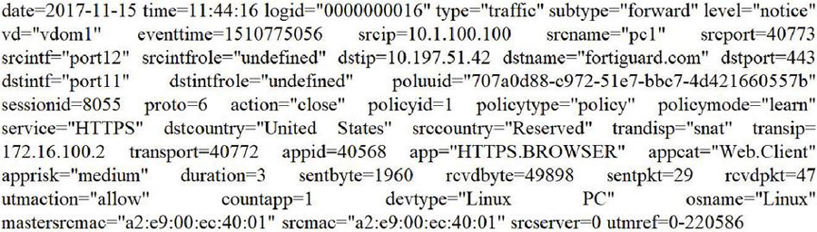
Figure 7 The content of the logs.txt file.
cat logs.txt |\
gsed -e ’s/\("\|[0-9]\) /\1|/g’ |\
awk -F’|’ ’{for(i=1; iNF; i++) {split($i,arr,"="); print "row:"NR "
attribute:"arr[1] " value:"arr[2] ;}}’
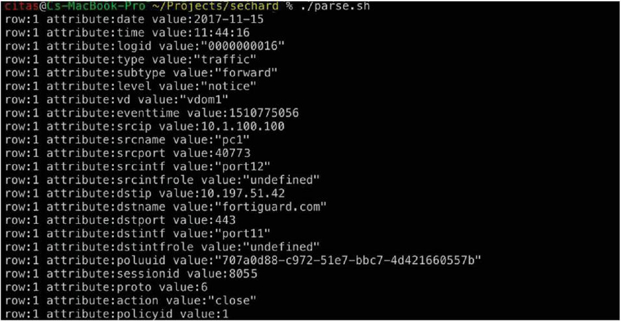
Figure 8 The output of the parse.sh given above.
In recent years, JavaScript Object Notation (JSON) has become a popular data interchange format. It is lightweight and has become the backbone of data communication in data science. An example Python code that can parse log files of Palo Alto firewalls and organise them in JSON format is given below. When the code is run, it produces output shown in Figure 9. This JSON data can then be used in machine learning processes. The code needs to be adjusted based on actual logs.
Content of the paloaltoparser.py:
import re
import json
import os
from collections import Counter
class PaloAltoLogParser:
def __init__(
self,
log_file_path="log_messages.json",
output_directory="parsed_fields/paloalto",
):
"""
Initialise PaloAltoLogParser class.
Parameters:
log_file_path (str): Path to the log messages JSON file.
output_directory (str): Directory to store parsed fields. Default is ’parsed_fields/paloalto’.
"""
self.log_file_path = log_file_path
self.output_directory = output_directory
def parse_log_messages(self):
"""
Parse log messages from the log file and write parsed data to JSON files.
"""
try:
# Load log messages from JSON file
with open(self.log_file_path, "r") as f:
data = json.load(f)
# Process each log message
for index, log_message_data in enumerate(data["log_messages"]):
log_message = log_message_data["message"]
description = log_message_data["description"]
# Extract header
header = log_message.split("||")[0]
# To match key−value pairs regular expression pattern
pattern = re.compile(r"(\w+)=([^ =]+)")
matches = pattern.findall(log_message)
# Convert matches to a dictionary
parameters = {key: value for key, value in matches}
# Create directory to store parsed data if not exists
os.makedirs(self.output_directory, exist_ok=True)
# Write parsed data to a JSON file
output_filename = os.path.join(
self.output_directory, f"parsed_fields_{index}.json"
)
with open(output_filename, "w") as f:
json.dump({"header": header, "parameters": parameters}, f, indent=4)
print(f"JSON file ’{output_filename}’ successfully created.")
print(f"Description: {description}")
print("All JSON files successfully created.")
except Exception as e:
print(f"An error occurred while parsing log messages: {e}")
def generate_key_statistics(self):
"""
Generate key statistics from parsed JSON files and save to a separate JSON file.
"""
try:
# Counter to store statistics of keys
key_statistics = Counter()
# Determine the upper limit of the loop dynamically
max_index = self.get_max_index()
# Read each JSON file and count keys
for i in range(max_index + 1): # Start from 0 to max_index inclusive
filename = os.path.join(
self.output_directory, f"parsed_fields_{i}.json"
)
with open(filename, "r") as f:
data = json.load(f)
parameters = data["parameters"]
key_statistics.update(parameters.keys())
Sample Palo Alto firewall log content (single message):
“Mar 1 21:06:08 xxx.xx.x.xx 3916 141 2021-03-01T21:06:08.438Z stream-logfwd20-587718190-03011255-ut6o-harness-5vlj logforwarder - panwlogs - CEF:0|Palo Alto Networks|LF|2.0|THREAT|file|3|ProfileToken=xxxxx dtz=UTC rt=Mar 01 2021 21:06:06 deviceExternalId=xxxxxxxxxxxxx PanOSConfigVersion= PanOSApplicationCategory=collaboration PanOSApplicationContainer= PanOSApplicationRisk=5 PanOSApplicationSubcategory=email PanOSApplicationTechnology=client-server PanOSCaptivePortal=false PanOSCloudHostname=PA-5220 PanOSCortexDataLakeTenantID=xxxxxxxxxxxxx PanOSDLPVersionFlag= PanOSDestinationDeviceClass= PanOSDestinationDeviceOS= dntdom= duser= duid= PanOSFileType=PNG File Upload PanOSInboundInterfaceDetailsPort=19 PanOSInboundInterfaceDetailsSlot=1 PanOSInboundInterfaceDetailsType=ethernet PanOSInboundInterfaceDetailsUnit=0 PanOSIsClienttoServer=false PanOSIsContainer=false PanOSIsDecryptMirror=false PanOSIsDecrypted= PanOSIsDuplicateLog=false PanOSIsEncrypted= PanOSIsIPV6= PanOSIsMptcpOn=false PanOSIsNonStandardDestinationPort=false PanOSIsPacketCapture=false PanOSIsPhishing=false PanOSIsPrismaNetwork=false PanOSIsPrismaUsers=false PanOSIsProxy=false PanOSIsReconExcluded=false PanOSIsSaaSApplication=false PanOSIsServertoClient=false PanOSIsSourceXForwarded= PanOSIsSystemReturn=false PanOSIsTransaction=false PanOSIsTunnelInspected=false PanOSIsURLDenied=false PanOSLogExported=false PanOSLogForwarded=true PanOSLogSource=firewall PanOSLogSourceTimeZoneOffset= PanOSNAT=false PanOSNonStandardDestinationPort=0 PanOSOutboundInterfaceDetailsPort=19 PanOSOutboundInterfaceDetailsSlot=1 PanOSOutboundInterfaceDetailsType=ethernet PanOSOutboundInterfaceDetailsUnit=0 PanOSPacket= PanOSProfileName= PanOSSanctionedStateOfApp=false PanOSSeverity=Low PanOSSourceDeviceClass= PanOSSourceDeviceOS= sntdom= suser= suid= PanOSThreatCategory= PanOSThreatNameFirewall= PanOSTunneledApplication=untunneled PanOSURL= PanOSUsers=xxx.xx.x.xx PanOSVirtualSystemID=1 start=Mar 01 2021 21:06:06 src=xxx.xx.x.xx dst=xxx.xx.x.xx sourceTranslatedAddress=xxx.xx.x.xx destinationTranslatedAddress=xxx.xx.x.xx cs1=dg-log-policy cs1Label=Rule suser0= duser0= app=smtp cs3=smtp cs3Label=VirtualLocation cs4=tap cs4Label=FromZone cs5=tap cs5Label=ToZone deviceInboundInterface=ethernet1/19 deviceOutboundInterface=ethernet1/19 cs6=test cs6Label=LogSetting cn1=4016143 cn1Label=SessionID cnt=9 spt=37404 dpt=25 sourceTranslatedPort=0 destinationTranslatedPort=0 proto=tcp act=alert filePath=page-icon.png cs2=any cs2Label=URLCategory flexString2=client to server flexString2Label=DirectionOfAttack externalId=xxxxxxxxxxxxx PanOSSourceLocation=xxx.xx.x.xx-xxx.xx.x.xx PanOSDestinationLocation=xxx.xx.x.xx-xxx.xx.x.xx fileId=0 PanOSFileHash= PanOSReportID= PanOSDGHierarchyLevel1=12 PanOSDGHierarchyLevel2=0 PanOSDGHierarchyLevel3=0 PanOSDGHierarchyLevel4=0 PanOSVirtualSystemName= dvchost=PA-5220 PanOSSourceUUID= PanOSDestinationUUID= PanOSIMSI=0 PanOSIMEI= PanOSParentSessionID=0 PanOSParentStartTime=Jan 01 1970 00:00:00 PanOSTunnel=N/A PanOSContentVersion= PanOSSigFlags=0 PanOSRuleUUID= PanOSHTTP2Connection= PanOSDynamicUserGroup= PanOSX-Forwarded-ForIP= PanOSSourceDeviceCategory= PanOSSourceDeviceProfile= PanOSSourceDeviceModel= PanOSSourceDeviceVendor= PanOSSourceDeviceOSFamily= PanOSSourceDeviceOSVersion= PanOSSourceDeviceHost= PanOSSourceDeviceMac= PanOSDestinationDeviceCategory= PanOSDestinationDeviceProfile= PanOSDestinationDeviceModel= PanOSDestinationDeviceVendor= PanOSDestinationDeviceOSFamily= PanOSDestinationDeviceOSVersion= PanOSDestinationDeviceHost= PanOSDestinationDeviceMac= PanOSContainerID= PanOSContainerNameSpace= PanOSContainerName= PanOSSourceEDL= PanOSDestinationEDL= PanOSHostID=xxxxxxxxxxxxxx PanOSEndpointSerialNumber=xxxxxxxxxxxxxx PanOSDomainEDL= PanOSSourceDynamicAddressGroup= PanOSDestinationDynamicAddressGroup= PanOSPartialHash= PanOSTimeGeneratedHighResolution=Jul 25 2019 23:30:12 PanOSReasonForDataFilteringAction= PanOSJustification= PanOSNSSAINetworkSliceType=”
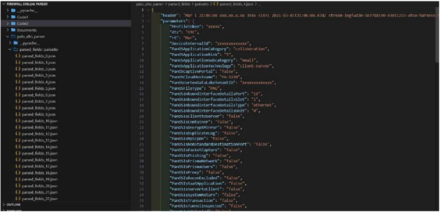
Figure 9 The output of Python code given above.
If the lines in Fortigate and Palo Alto firewalls are considered, it can be seen that “src” corresponds to “srcip” and “dst” corresponds to “dstip”. The following lines can be included in the prepared script to change “srcip” to “src” and “dstip” to “dst”. Unluckily, there is no one-fits-all solution that is suitable for parsing any types of logs from different brands.
cd /nameofthedirectory
grep -RiIl ’srcip’ |xargs sed -i ’s/srcip/src/g’
grep -RiIl ’dstip’ |xargs sed -i ’s/dstip/dst/g’
From the log file, it is possible to fetch the IP addresses following “src=”.
grep ’src=’ logfile.txt |awk -F ’|’ ’{print $2}’
As an alternative to grep based scripts, awk or sed can be used. As it can be understood, Linux offers various commands and tools to handle log files.
awk -F ’|’ ’/^src=/{print $2}’ logfile.txt
sed -n ’s/^src *|//p’ logfile.txt
6 Conclusion
In this study, firewall log files were classified using different classification algorithms and the performances of the algorithms were evaluated by using a selected set of performance metrics. Among the set of performance metrics, we particularly focused on the MCC because the MCC offers reliable results when a dataset does not consist of equal or proportional number of instances belonging to each class. It can be seen when the performance metrics were examined that the highest average MCC values were achieved when the BF tree, the FT tree, the J48, the NB tree and the Simple Cart algorithms were used. In particular, the Simple Cart algorithm made the best predictions for the reset-both class, which was not predicted successfully by the other algorithms. Therefore, using the Simple Cart algorithm is recommended to classify firewall log files. The use of log files of a single firewall brand is the limitation of this study. As a future work of this study, we both plan to use log files of multiple firewall brands and propose an approach to integrate the classification of firewall log files into honeypot and honeynet systems so that potential threats can be better modelled.
References
[1] Karen, S., and H. Paul. 2008. Guidelines on firewalls and firewall policy, NIST Recommendations, SP, p. 800–841.
[2] Kent, K., and M. Souppaya. 2006. Guide to computer security log management: recommendations of the National Institute of Standards and Technology, US Department of Commerce, Technology Administration.
[3] Ertam, F., and M. Kaya. 2018. Classification of firewall log files with multiclass support vector machine, 2018 6th International symposium on digital forensic and security (ISDFS), IEEE, p. 1–4.
[4] González-Granadillo, G., S. González-Zarzosa, and R. Diaz. 2021. Security information and event management (siem): Analysis, trends, and usage in critical infrastructures, Sensors, 21, 4759.
[5] Al-Haija, Q.A., and A. Ishtaiwi. 2022. Multiclass Classification of Firewall Log Files Using Shallow Neural Network for Network Security Applications, Soft Computing for Security Applications, Springer, p. 27–41.
[6] Chicco, D., and G. Jurman. 2020. The advantages of the Matthews correlation coefficient (MCC) over F1 score and accuracy in binary classification evaluation, BMC genomics, 21: 1–13.
[7] Arnaldo, I., A. Cuesta-Infante, A. Arun, M. Lam, C. Bassias, and K. Veeramachaneni. 2017. Learning representations for log data in cybersecurity, International conference on cyber security cryptography and machine learning, Springer, p. 250–268.
[8] Lu, J., F. Lv, Z. Zhuo, X. Zhang, X. Liu, T. Hu, and W. Deng. 2019. Integrating traffics with network device logs for anomaly detection, Security and Communication Networks, 2019: 1–10.
[9] Ucar, E., and E. Ozhan. 2017. The analysis of firewall policy through machine learning and data mining, Wireless Personal Communications, 96: 2891–2909.
[10] Gutierrez, R.J., K.W. Bauer, B.C. Boehmke, C.M. Saie, T.J. Bihl. 2018. Cyber anomaly detection: Using tabulated vectors and embedded analytics for efficient data mining, Journal of Algorithms & Computational Technology, 12: 293–310.
[11] Yang, G., Y. Zhao, B. Li, Y. Ma, R. Li, J. Jing, and Y. Dian. 2019. Tree species classification by employing multiple features acquired from integrated sensors, Journal of Sensors, 2019: 1–12.
[12] Keerthi, S.S., S.K. Shevade, C. Bhattacharyya, and K.R.K. Murthy. 2001. Improvements to Platt’s SMO algorithm for SVM classifier design, Neural computation, 13: 637–649.
[13] Altman, N.S. 1992. An introduction to kernel and nearest-neighbor nonparametric regression, The American Statistician, 46: 175–185.
[14] Aha, D.W., D. Kibler, and M.K. Albert. 1991. Instance-based learning algorithms, Machine learning, 6: 37–66.
[15] Quinlan, J.R. 1987. Simplifying decision trees, International journal of man-machine studies, 27: 221–234.
[16] Srinivasan, D.B., and P. Mekala. 2014. Mining social networking data for classification using reptree, International Journal of Advance Research in Computer Science and Management Studies, 2(10): 155–160.
[17] Kalmegh, S. 2015. Analysis of weka data mining algorithm reptree, simple cart and randomtree for classification of indian news, International Journal of Innovative Science, Engineering & Technology, 2: 438–446.
[18] Pfahringer, B. 2010. Random model trees: an effective and scalable regression method.
[19] Landwehr, N., M. Hall, E. Frank. 2005. Logistic model trees, Machine learning, 59: 161–205.
[20] Geurts, P., D. Ernst, and L. Wehenkel. 2006. Extremely randomized trees, Machine learning, 63: 3–42.
[21] Hulten, G., L. Spencer, and P. Domingos. 2001. Mining time-changing data streams, Proceedings of the seventh ACM SIGKDD international conference on Knowledge discovery and data mining, p. 97–106.
[22] Tan, C., H. Chen, and C. Xia. 2009. The prediction of cardiovascular disease based on trace element contents in hair and a classifier of boosting decision stumps, Biological trace element research, 129: 9–19.
[23] Coºkun, C., and A. Baykal. 2011. An application for comparison of data mining classification algorithms, XIII. Akademik Biliþim Konferansı, p. 51–58.
[24] Gama, J. 2004. Functional trees, Machine learning, 55: 219–250.
[25] Shi, H. 2007. Best-first decision tree learning, The University of Waikato.
[26] Kohavi, R. 1996. Scaling up the accuracy of naive-bayes classifiers: A decision-tree hybrid, Kdd, 202–207.
[27] Frank, E. 2014. Fully supervised training of Gaussian radial basis function networks in WEKA.
[28] Holmes, G., B. Pfahringer, R. Kirkby, E. Frank, and M. Hall. 2002. Multiclass alternating decision trees, European Conference on Machine Learning, Springer, p. 161–172.
[29] Freund, Y., and R.E. Schapire. 1996. Experiments with a new boosting algorithm, icml, Citeseer, 148–156.
[30] Joshi, R. 2016. Accuracy, precision, recall & f1 score: Interpretation of performance measures, Retrieved April, 1, 2022.
[31] Eibe, F., M.A. Hall, and I.H. Witten. 2016. The WEKA workbench. Online appendix for data mining: practical machine learning tools and techniques, Morgan Kaufmann, Elsevier Amsterdam, The Netherlands.
[32] Kotthoff, L., C. Thornton, H.H. Hoos, F. Hutter, and K. Leyton-Brown. 2019. Auto-WEKA: Automatic model selection and hyperparameter optimization in WEKA, Automated Machine Learning, Springer, Cham, 81–95.
[33] Bilalli, B., A. Abelló, T. Aluja-Banet, and R. Wrembel. 2016. Automated data pre-processing via meta-learning, International Conference on Model and Data Engineering, Springer, p. 194–208.
[34] As-Suhbani, H.E., and S. Khamitkar. 2018. Mining Frequent Patterns in Firewall Logs Using Apriori Algorithm with WEKA, International Conference on Recent Trends in Image Processing and Pattern Recognition, Springer, p. 561–571.
[35] Astekin, M., S. Özcan, and H. Sözer. 2019. Incremental analysis of large-scale system logs for anomaly detection in 2019 IEEE International Conference on Big Data (Big Data). IEEE.
[36] Xiao, T., et al., LPV: A Log Parsing Framework Based on Vectorization. IEEE Transactions on Network and Service Management, 2023.
[37] Xiao, T., et al. 2020. Lpv: A log parser based on vectorization for offline and online log parsing. in 2020 IEEE International Conference on Data Mining (ICDM). IEEE.
[38] Lashram, A.B., L. Hsairi, and H. Al Ahmadi, 2023. HCLPars: A New Hierarchical Clustering Log Parsing Method. Engineering, Technology & Applied Science Research, 13(4): p. 11130–11138.
[39] Coustié, O., et al. 2020. Meting: A robust log parser based on frequent n-gram mining. in 2020 IEEE International Conference on Web Services (ICWS). IEEE.
[40] Chunyong, Z. and X. Meng. 2020. Log parser with one-to-one markup. in 2020 3rd International Conference on Information and Computer Technologies (ICICT). IEEE.
[41] Zhang, S., et al., 2020. Efficient and robust syslog parsing for network devices in datacenter networks. IEEE access, 8: p. 30245–30261.
[42] Bai, Y., Y. Chi, and D. Zhao, 2023. PatCluster: A Top-Down Log Parsing Method Based on Frequent Words. IEEE Access, 11: p. 8275–8282.
[43] Liu, X., Y. Zhu, and S. Ji. 2020. Web log analysis in genealogy system. in 2020 IEEE International Conference on Knowledge Graph (ICKG). IEEE.
[44] Liu, W., et al. 2020. FastLogSim: A quick log pattern parser scheme based on text similarity. in International Conference on Knowledge Science, Engineering and Management. Springer.
[45] Vervaet, A., et al., 2024. Online log parsing using evolving research tree. Knowledge and Information Systems, 66(2): p. 1231–1255.
[46] Le, V.-H. and H. Zhang, 2023. An evaluation of log parsing with chatgpt. arXiv preprint arXiv:2306.01590.
[47] Yu, S., et al., 2023. Self-supervised log parsing using semantic contribution difference. Journal of Systems and Software, 200: p. 111646.
[48] Chen, X., et al., 2023. AS-Parser: Log Parsing Based on Adaptive Segmentation. Proceedings of the ACM on Management of Data, 1(4): p. 1–26.
[49] Xu, J., et al. 2023.Hue: A user-adaptive parser for hybrid logs. in Proceedings of the 31st ACM Joint European Software Engineering Conference and Symposium on the Foundations of Software Engineering.
[50] El-Masri, D., et al., 2020. A systematic literature review on automated log abstraction techniques. Information and Software Technology, 122: p. 106276.
[51] Zhu, J., et al. 2019. Tools and benchmarks for automated log parsing. in 2019 IEEE/ACM 41st International Conference on Software Engineering: Software Engineering in Practice (ICSE-SEIP). IEEE.
Biographies

Ebru Efeoğlu is currently an Assistant Professor at Kutahya Dumlupinar University Software Department. She received her B.Sc. degree in Geophysics Engineering from Kocaeli University and Management Information Systems from Anadolu University, Turkey. She received her Ph.D. degree in Computer Engineering from Trakya University, Turkey in 2021. She has authored several papers in international conference proceedings and SCI-Expanded journals. Her research interests include machine learning and data mining, and their applications in various research domains.

Gurkan Tuna is currently a Professor at the Department of Computer Programming at Trakya University, Turkey. He is also the head of the graduate program of Mechatronics Engineering at the same university. His current research interests include wireless networks, wireless sensor networks, and data security.
Journal of Web Engineering, Vol. 23_4, 561–594.
doi: 10.13052/jwe1540-9589.2344
© 2024 River Publishers