Towards Adaptive Continuous Trajectory Clustering Over a Distributed Web Data Stream
Yang Wu1, Junhua Fang1,*, Pingfu Chao1, Zhicheng Pan2, Wei Chen1 and Lei Zhao1
1School of Computer Science and Technology, Soochow University, China
2School of Data Science and Engineering, East China Normal University, Shanghai, China
E-mail: 20215227099@stu.suda.edu.cn; jhfang@suda.edu.cn, pfchao@suda.edu.cn; 52265903002@stu.ecnu.edu.cn; robertchen@suda.edu.cn, zhaol@suda.edu.cn
*Corresponding Author
Received 14 September 2022; Accepted 27 November 2022; Publication 14 April 2023
Abstract
With the popularity of modern mobile devices and GPS technology, big web stream data with location are continuously generated and collected. The sequential positions form a trajectory, and the clustering analysis on trajectories is beneficial to a wide range of applications, e.g., route recommendation. In the past decades, extensive efforts have been made to improve the efficiency of static trajectory clustering. However, trajectory stream data is received incrementally, and the continuous trajectory clustering inevitably faces the following two problems: (1) physical structure design for trajectory representation leads to severe space overhead, and (2) dynamic maintenance of trajectory semantics and its retrieval structure brings intensive computation. To overcome the above problems, an adaptive continuous trajectory clustering framework (ACTOR) is proposed in this paper. Overall, it covers three key components: (1) Simplifier represents trajectory with a well-designed PT structure. (2) Partitioner utilizes a hexagonal-based indexing strategy to enhance the local computational efficiency. (3) Executor accommodates an adaptive selection of P-clustering and R-clustering approaches according to the ROC (rate of change) matrix. Empirical studies on real-world data validate the usefulness of our proposal and prove the huge advantage of our approach over available solutions in the literature.
Keywords: Spatio-temporal data, continuous trajectory clustering, distributed stream processing, trajectory analysis.
1 Introduction
In recent years, with the rapid development of sensor technology and smartphones, GPS devices are widely applied to track moving objects [3, 16], which can produce numerous location data every moment. For instance, an Uber car reports its location every few seconds. As a result, applications from different domains collect substantial amounts of location data and form a trajectory. Analyzing trajectories as they are generated will benefit a variety of modern applications, such as carpooling [15] and route recommendation [23].
Trajectory clustering aims to group a large number of trajectories into several relatively homogeneous clusters [10, 18, 22], which plays a crucial role in trajectory analysis since it reveals underlying trends of moving objects. Figure 1(a) is a naive example to demonstrate trajectory clustering, which indicates representative paths and potential motion trends.
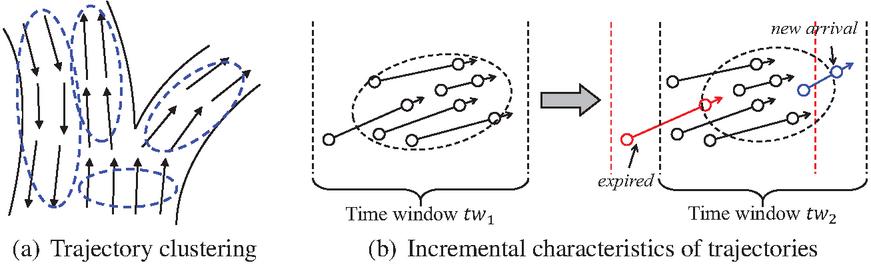
Figure 1 An example of trajectory clustering and incremental characteristic of trajectories.
Existing traditional trajectory clustering algorithms [11, 12, 1, 15] adopt a specific similarity metric to cluster trajectories in a centralized environment on static datasets. However, due to their sequential nature, trajectory data are often received incrementally, e.g., continuous new points are reported by the GPS system. Figure 1(b) depicts the incremental characteristics of trajectories, where we employ a time window to limit the trajectory stream to a specified set of records within a given time horizon. We find that part of the state information (i.e., unexpired points) in time window is still stored in time window . So it is significant to select a suitable data structure to maintain the previous state information dynamically. Therefore, continuous trajectory clustering is more suitable for such incremental scenarios. Once the trajectories are received, we analyze them to better understand the current cluster patterns and their evolution between successive periods of time [13]. Moreover, the continuous clustering of trajectories over vast volumes of streaming data has been recognized as critical for many modern applications. Since a broad spectrum of applications that rely on trajectory clustering are time-sensitive, it is essential to utilize an incremental computing mode to perform continuous clustering on large-scale trajectory data in a real-time manner to maximize its application value [23].
Nowadays, an increasing number of works are devoted to the study of continuous trajectory clustering. TCMM [17] is a continuous trajectory clustering framework. Nevertheless, it cannot clear the expired data, thus it is not suitable for large-scale datasets, and the accumulation of expired data will reduce the clustering quality. Both CUTiS [7] and TSCluWin [18] achieve continuous clustering by maintaining a space-consuming data structure within the sliding window. They comprehensively integrate the trajectory features, and it takes a great deal of time to maintain and update the cluster information. In our previous work [21], we proposed a real-time trajectory clustering framework Lunatory. Although the framework has high real-time performance, it does not take advantage of the incremental characteristics of trajectories.
As observed above, continuous trajectory clustering is challenging and existing methods suffer extensive limitations. Therefore, we divide the realization of this operator into the following three requirements:
1. Physical structure design for trajectory representation (R1): The structure of representing trajectories directly affects the cross-node transmission and computational efficiency of clustering operators. However, the compression/simplification of the trajectory needs to be adapted to the specific trajectory clustering algorithm, and it is extremely difficult to obtain a high-accuracy and efficient trajectory clustering ability with minimal information loss.
2. Dynamic maintenance of the trajectory semantic (R2): Trajectory is a dynamic sequence. For the continuous trajectory clustering operator, there will be continuous expiration and generation of position points. A reasonable maintenance strategy needs to be designed to delete expired elements. If expired elements continue to accumulate, the quality of the clustering results will deteriorate.
3. Dynamic maintenance of the retrieval structure (R3): Partitioning and indexing techniques can improve the local computing efficiency of clustering, but also cause a certain update overhead. There is no free lunch in this world, and how to achieve satisfactory efficiency at a small cost is a difficult point in designing a complex trajectory clustering framework.
According to the above requirements, we propose ACTOR, an adaptive continuous trajectory clustering framework. Specifically, the major contributions of this paper include:
1. We propose a continuous trajectory clustering framework ACTOR by extending our previous work [21] to achieve accurate and efficient continuous clustering in an incremental and real-time scenario.
2. To answer R1, we propose an MDL-based trajectory simplification algorithm to characterize the feature information of the trajectory. Then we compress the simplified trajectory into a pivot trajectory.
3. To answer R2 and R3, we propose two sophisticated clustering approaches (i.e., P-clustering and R-clustering) and introduce the ROC matrix for the adaptive selection of appropriate clustering approach.
4. We implement all proposed methods on top of Flink. Empirical studies on real-world data validate the usefulness of our proposal and prove competitive performance over state-of-the-art solutions in the literature.
The rest of this paper is organized as follows. In Section 2, we introduce the clustering algorithm based on points and trajectories. We then present the preparatory knowledge for designing ACTOR in Section 3. We present the overall framework of ACTOR in its entirety in Section 4 and describe the details of each process in the framework. We analyse the experimental results in Section 5 and finally, we conclude our proposal in brief in Section 6.
2 Related Work
2.1 Point Clustering
There are currently various clustering algorithms, and here we choose the density-based clustering algorithm, which is the same as the one we used in [4]. The high-density data belonging to the same cluster is the basic idea of the density-based clustering algorithm [23]. The typical ones include DBSCAN [9], OPTICS [2] and mean-shift [5]. DBSCAN [9] finds the largest set of points of any shape that are density-connected by the radius and the minimum number of points , but if the densities between clusters are different, the clustering results will significantly deteriorate. ST-DBSCAN [3] extends DBSCAN to be able to discover clusters on spatial–temporal data. In their work [3], the authors introduce a new density factor that represents the density of the cluster. It makes up for the disadvantage that DBSCAN cannot cluster points with different densities. However, these point-based algorithms do not consider the state information of a trajectory [23]. It makes it hard for them to be applied to trajectory clustering directly.
2.2 Stateless Trajectory Clustering
On top of point-based clustering algorithms, existing trajectory clustering methods can be roughly divided into two categories: partition-based [11, 12] and density-based [1, 15, 17]. The methods mentioned above usually cluster the entire trajectory on a static dataset, without considering the state maintenance of trajectories in the incremental scenario. TRACLUS [15] first partitions trajectories into trajectory segments, and then perform a density-based clustering algorithm between trajectory segments. However, this algorithm cannot effectively handle incremental data in streaming environments. Chen et al. [4] propose a real-time distributed trajectory clustering framework Disatra, in which a data structure AT was introduced to describe the trajectory characteristics. Inspired by TRACLUS, Disatra uses a density-based clustering algorithm for AT to generate clusters. Although Disatra extends trajectory clustering to the real-time environment, the accuracy of the clustering results is not satisfactory due to the huge information loss in the process of its radical trajectory compression, i.e. abstract trajectory. In our previous work [21], we simplified the trajectory and then utilized the pivot trajectory to represent the simplified trajectory segment. After that, we adopted a hexagonal-based indexing strategy to index the pivot trajectory, and finally, we implemented the PT-based DBSCAN clustering algorithm. Although the framework improves the clustering quality based on meeting the real-time requirements, it clusters all pivot trajectories from scratch on each time window without considering the incremental characteristics of trajectories.
2.3 Continuous Trajectory Clustering
Since the trajectories are coordinate points with a time sequence [14], continuous trajectory clustering aims to maintain the information of clusters before the current time by utilizing a certain data structure [19, 13]. The TCMM [17] framework consists of two parts: online micro-cluster maintenance and offline macro-cluster creation. Online micro-clustering maintains a data structure called cluster features (CF), which stores statistical information of similar trajectory segments. However, the framework does not regularly remove obsolete data, so while continuously absorbing trajectory records for clustering and merging, it will lead to the shift of the micro-cluster center and reduce the effectiveness of the resulting cluster. Inspired by TCMM, trajectory stream clustering over a sliding window framework TSCluWin was proposed by Mao et al. [18]. They design two data structures to represent the spatial features of trajectories and finally cluster streaming trajectories over a sliding window using TSCluWin. Since this framework comprehensively incorporates the features of trajectories and also creates macro-clusters based on micro-clusters, it is expected to be time-consuming. CUTiS [6, 7] is an incremental algorithm for a trajectory data stream, which uses a micro group structure to maintain the cluster information of moving objects in continuous time windows. Although the overhead of the algorithm will be lower than the cost of running the clustering algorithm from scratch, the definition of the micro group is based on the representative trajectory, and it still needs to pay extra expenses in the process of calculation and maintenance.
3 Preliminary
In this section, we will introduce the definition of our continuous trajectory clustering problem. To begin with, we first list all notations frequently used in our paper, as shown in Table 1:
Table 1 Summary of notations
| Notation | Description |
| Trajectory consisting of points. | |
| A sampling point that forms the trajectory. | |
| A set of trajectory segments. | |
| A trajectory segment in . | |
| Distance threshold between pivot trajectories. | |
| Minimum number in -neighborhood. | |
| The -neighborhood of trajectory segment . | |
| A set of pivot trajectories. | |
| Pivot trajectory. |
Definition 1 (Trajectory). A trajectory is a series of chronologically ordered points , representing the trace of a moving object. Each point denotes the object’s location at time stamp , and a line connecting two adjacent points is defined as a trajectory segment .
Although distance metrics like DTW and LCSS are widely used to measure the similarity between trajectories, since these methods are sensitive to trajectory length and sampling rate, we utilize the following trajectory distance to calculate the distance between two trajectories.
Definition 2 (Trajectory distance). Given two trajectory segments and , the start and end points of trajectory segment are and . Similarly, the start and end points of trajectory segment are and , respectively. Assuming that , the trajectory distance between two trajectory segments is defined as .
Here, the weights , , and can be adjusted as needed. We set these weights to 1 by default. An example of trajectory distance is given in Figure 2.
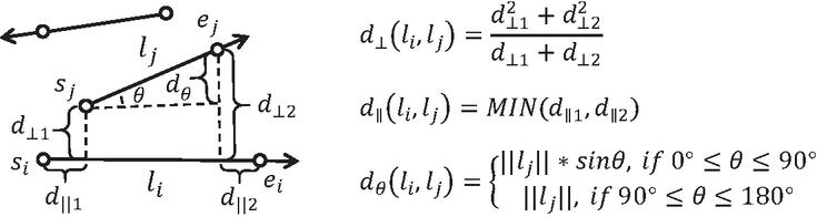
Figure 2 Trajectory distance.
Definition 3 (Pivot trajectory). A compact synopsis data structure pivot trajectory is defined to describe the moving characteristics of a trajectory segment. Among them, represents the center point of a trajectory segment, denotes the deflection angle of the trajectory segment, and are the bottom left corner and top right corner of the MBR (minimal bounding rectangle) enclosing the trajectory segment, respectively, and represents the time stamp of the most recent trajectory segment.
Definition 4 (Time window). A trajectory stream is an infinite sequence of chronologically ordered points, and we employ a time window to limit the trajectory stream to a specified finite set of trajectories within a given time range. The start time of the time window is , the end time is , and the trajectory set can be obtained within the time window.
4 Framework Design and Implementation
4.1 Overview of ACTOR
ACTOR is a distributed clustering framework built on Flink, which aims to achieve high-quality continuous trajectory clustering in real-time. Overall, ACTOR consists of three phases: pivot trajectory generation, hexagonal-based partitioning and clustering execution (including monitoring of ROC matrix, P-clustering and R-clustering), as shown in Figure 3. We will explain the meaning of each component later.
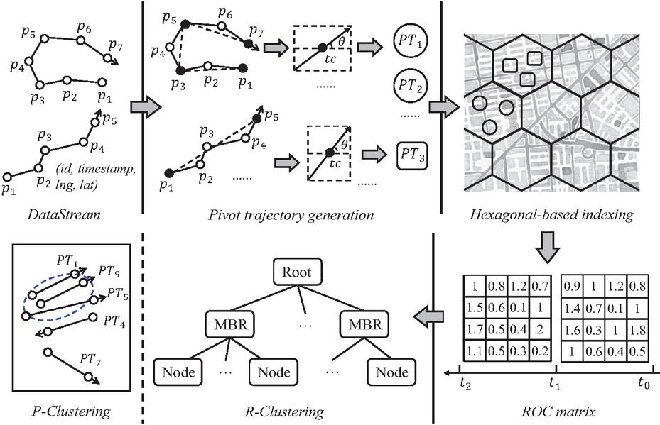
Figure 3 Framework of ACTOR.
PT generation. We employ the MDL principle to simplify the trajectory and abstract the simplified trajectory segment as a pivot trajectory. First, we simplify the trajectory of a moving object. The purpose is to represent the trajectory with the least points while preserving the moving characteristics of the trajectory as much as possible. Ultimately, it can significantly reduce the computation cost while ensuring the accuracy of clustering results. The trajectory characteristics are extracted from the simplified trajectory segment to form . Since the contains a bounding box enclosing the simplified trajectory segment, partitioning the pivot trajectory ensures a trajectory segment will not cross multiple partitions. Therefore, it reduces data redundancy and improves the utilization of node resources.
Hexagonal-based indexing. To avoid cross-node data transmission in a distributed environment, we adopt the hexagonal-based partitioning strategy to send with the same coding value to the same partition. At the same time, an overlap algorithm is designed to send pivot trajectories around the margin of a partition to its adjacent partitions, which improves the accuracy of clustering results while reducing the data transmission to the greatest extent.
Clustering execution. It contains two main steps:
(1) Monitoring the ROC matrix: In each partition, we count the sum of new and expired PTs in the current time window, divide it by the number of PTs in the previous time window to get the rate of change in the current time window. The appropriate clustering method is adaptively selected according to the ROC corresponding to each partition.
(2a) P-clustering: We perform PT-based DBSCAN clustering on pivot trajectories in the same partition within a time window to obtain the clustering results. The aforementioned clustering process is performed in each distributed node.
(2b) R-clustering: We employ an R-tree in each partition to dynamically maintain the core trajectory segments in the cluster. The new PT is searched in the R-tree to determine whether there are clusters to join. At the same time, the R-tree needs to be periodically adjusted to delete the expired data. Finally, the clustering results in each node are collected to form final clusters.
4.2 Pivot Trajectory Generation
In the real-time environment, extracting detailed or concise trajectory characteristics is a trade-off between high accuracy and low runtime. On the one hand, the higher the preciseness, the more complete the moving characteristics of the entire trajectory can be retained, as shown in Figure 4(b). On the other hand, the higher the conciseness, the fewer trajectory segments are used to represent the trajectory, and the higher the node resource utilization rate is, as depicted in Figure 4(c). Therefore, we use the MDL (minimum description length) principle [20] to find the optimal partition of the trajectory, as shown in Figure 4(a). Then the pivot trajectory (i.e. PT) is utilized to characterize the simplified trajectory, which reduces data redundancy and improves the utilization of node resources.
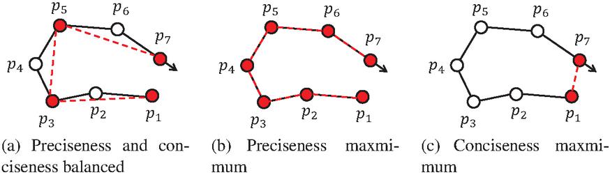
Figure 4 Examples of trajectory simplification.
Suppose a trajectory and a set of characteristic points . Every two adjacent characteristic points form a line segment . We use the two formulas mentioned in TRACLUS [15]:
| (1) | |
| (2) |
Equation 1 measures the degree of conciseness, and Equation 2 measures the degree of preciseness. Here, denotes the Euclidean distance between and . For example, in Figure 4(a), the formulas of and between and are as follows:
| (3) | |
| (4) |
We utilize Equation 5 to denote the MDL cost of a trajectory between and when assuming that is a simplified trajectory segment, and Equation 6 denotes the MDL cost when assuming that we don’t need to simplify the trajectory , i.e., we preserve the original trajectory.
| (5) | |
| (6) |
A finite-length trajectory is simplified using the MDL principle, as shown in Algorithm 1. We compute and for each point in a trajectory (lines 5, 6). If , we simplify the trajectory from to to and add to the set (lines 8–11). Otherwise, we increase the length of a candidate trajectory segment (line 13).
Algorithm 1 MDL-based trajectory simplification
Input: Sampling points
Output: A set of pivot trajectories
1 Initialize ;
2 start = 1, length = 1;
3 while start + length do
4 curr = start + length;
5 ;
6 ;
7 if then
8 Update ;
9 Add to set ;
10 start = curr - 1, length = 1;
11 Initialize ;
12 else
13 length = length + 1;
14 Update ;
15 Add to set ;
Next, we calculate for each trajectory segment . Since consists of two sampling points, it is easy to calculate the trajectory segment center point , the deflection angle , the bottom left corner and the top right corner of the MBR enclosing . We use the timestamp of the trajectory segment end point to represent the time , which records the last timestamp of the current time window.
4.3 Hexagonal-based Partitioning Strategy
The grid system is essential for analyzing massive spatial data sets and dividing the earth’s space into identifiable grid cells. In a grid-based spatial system, the more polygonal sides are used, the more a grid approximates a circle, and the more convenient it is to perform kNN query, etc. However, grid indexing requires the space to be filled with grids without gaps. It proves that the only shapes used for grid spatial indexing are triangles, rectangles, and hexagons. Hexagons [8] have the most sides and are the closest to a circle, so in theory, they are the best choice in certain scenarios.
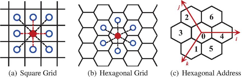
Figure 5 Square grid and hexagonal grid.
We further elaborate on the difference between the square and hexagonal grid. As shown in Figure 5, a hexagonal grid has only one type of distance between a hexagon center point and its neighbors, whereas there are two types of distance (marked as red and black) for a square grid. This property greatly simplifies the process of performing analysis and smoothing over gradients.
In general, for different levels of address generation, each hexagon contains the address of its parent hexagon. In this way, only the calculation method of the sub-grid address of each grid needs to be specified. For the sub-grid, it is only necessary to append the address of the sub-grid after the coordinates of its parent grid.
We encode from via H3 encoding and send to a corresponding partition according to the encoding value of . Since we compress the simplified trajectory segment into a data structure PT with the midpoint of the trajectory segment, our index will not produce cross-partition data so that we can avoid the problem of cross-node data transmission in a distributed environment.
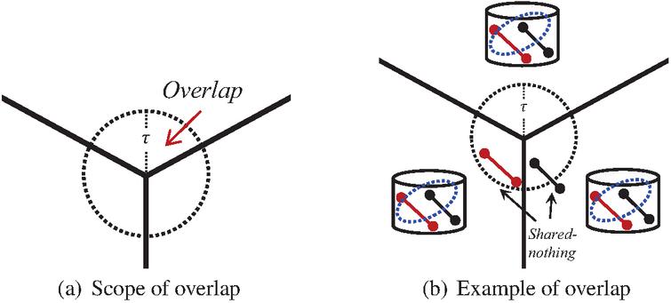
Figure 6 Overlap mechanism.
However, in the process of clustering, some extreme cases may occur. For example, the pivot trajectories in the same cluster are divided into different partitions, and these pivot trajectories are around the margin of the partition, which leads to the reduction of clustering accuracy. Therefore, we design a hexagon-based overlap mechanism. As shown in Figure 6(a), we take the vertex of each hexagonal partition as the center of the circle, and draw an area with the radius of . For the whose falls within this range, we distribute it to two adjacent partitions and execute the clustering algorithm, respectively. The non-optimized cross-node data transmission will send the data to all other nodes. On the contrary, our overlap mechanism only needs to send data to the two partitions participating in the overlap, which minimizes the data transmission and data redundancy while improving the algorithm efficiency. Figure 6(b) shows an example of the overlap. The red and black are expected to be in the same cluster. With the help of the overlap mechanism, the red is sent to the partition containing , or vice versa, depending on which partition performs the clustering first.
4.4 Clustering Execution
4.4.1 ROC matrix
Since our framework contains two clustering approaches: P-clustering and R-clustering, it is worth considering which approach to choose under what circumstances. A new batch of data will be received in each time window, and the data in the window will be reclustered in any case according to P-clustering. While R-clustering will search in the R-tree to determine whether the new can be allocated to a cluster and dynamically maintain the R-tree.
Although the average time complexity of searching, inserting, and deleting items of the R-tree is lower than that of P-clustering, when there are substantial new and expired data in a time window, the maintenance cost of the R-tree will inevitably rise. At this time, P-clustering may be better than R-clustering. Therefore, we design a ROC matrix (i.e., rate of change matrix), which in each partition counts the sum of new and expired PTs in the current time window, dividing it by the number of PTs in the previous time window to obtain the rate of change. The appropriate clustering method is adaptively selected through the ROC corresponding to each partition. The setting of ROC threshold is not set in stone. The threshold is scalable, and users can adjust it for various datasets to get excellent performance in different scenarios. According to Section 5.2, we set the threshold to , that is, when the ROC is greater than , we adopt P-clustering. Instead, we perform R-clustering to process pivot trajectories incrementally.
4.4.2 P-clustering
Since the pivot trajectories have both direction and length, which lead to arbitrary shapes of the clusters, we choose the density-based clustering method. Inspired by the idea of DBSCAN, Lee et al. [15] propose a line segment clustering algorithm. Similarly, we apply segment clustering to pivot trajectory within the current time window.
The trajectory distance is given in creftypecap 2. Next, relevant concepts in PT-based DBSCAN clustering (P-clustering for short) are introduced:
(1) Core trajectory segment: Using the trajectory distance in creftypecap 2, we can calculate the number of trajectory segments whose distance from is less than or equal to the threshold . When is greater than , we call the trajectory segment as the core trajectory segment, and define as .
(2) Directly density-reachable: Given two trajectory segments , if is a core trajectory segment and , we say the trajectory segment is directly density-reachable from the trajectory segment .
(3) Density-reachable: Given a chain of trajectory segments , , if is directly density-reachable from , we call the trajectory segment is density-reachable to the trajectory segment .
(4) Density-connected: Given two trajectory segments , if there is a trajectory segment such that both and are density-reachable from , we call the trajectory segment is density-connected from the trajectory segment .
Algorithm 2 P-clustering
Input: A set of pivot-trajectories ,
time window range , two parameters and
Output: A set of clusters
1 Initialize cluster ID to be 1;
2 Mark pivot trajectories in as unclassified;
3 for do
4 if is unclassified then
5 if then
6 Set cluster ID to ;
7 Insert into a queue ;
8 while do
9 Get a ;
10 if then
11 for do
12 if is unclassified or a noise then
13 Set cluster ID to ;
14 Insert to the queue ;
15 Remove ;
16 cluster ID := cluster ID + 1;
17 else
18 noise
Algorithm 2 describes the process of clustering PTs employing the idea of DBSCAN. Lines – and – of the algorithm judge whether a is a core trajectory segment. If is determined as a core trajectory segment, the algorithm will continue to execute lines –. Otherwise, the is judged as a noise. Lines –, the algorithm computes the density-connected set of a core trajectory segment.
We perform the real-time clustering to all pivot trajectories in the same time window. For in a partition, we randomly select an unclassified and judge whether is a core trajectory segment through trajectory distance and parameters, i.e., and . If is the core trajectory segment, we continue to find all pivot trajectories density-connected with , and finally we set them as classified and assign the same cluster number to them. Otherwise, it is temporarily classified as noise. We repeat the above steps until all are classified.
4.4.3 R-clustering
In the process of continuous trajectory clustering, we need to adopt a data structure to maintain the state of clusters and trajectories in the time window. Since we abstract the trajectory segment into pivot trajectory (including trajectory segment midpoint), and a core trajectory segment must correspond to a cluster, so we choose the R-tree to maintain the core trajectory segment, and perform continuous clustering on R-tree. In Figure 7, the core trajectory segments in each grid are maintained by an R-tree. The newly arrived PT is searched on the R-tree to observe whether it belongs to a certain cluster.
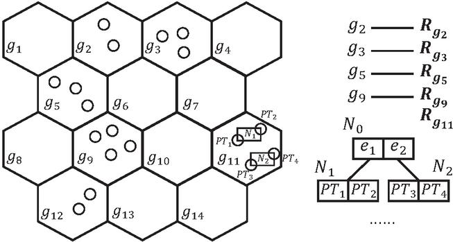
Figure 7 Continuous clustering based on an R-tree.
The R-clustering can be divided into the following two cases:
(1) New PT added. For the new arrival of the pivot trajectory in the time window, we search the R-tree for the node whose trajectory distance from is less than or equal to . If such a node can be retrieved in the R-tree, we assign the cluster ID of the represented by the node to . The reason is that if the trajectory distance between and is less than or equal to , then is in the , so they must belong to the same cluster. If we cannot retrieve such a node in the R-tree, we should not immediately treat as noise, but add it to a list that dynamically maintains that does not belong to any cluster within the time window. Whenever the number of in the list reaches or an integer multiple of , we implement P-clustering to in the list. If the elements in the list can form one or more clusters, we add the core trajectory segments to the R-tree and remove the s assigned to the cluster ID from the list. Note that in the process of clustering, it is necessary to determine whether the in the list has expired, that is, if it is not within the time window. If the has expired, it should be removed from the list in time.
(2) Expired PT deleted. For the expired pivot trajectory in the time window, we need to remove it from the R-tree. As time goes on, more and more expired will accumulate in the R-tree, and the nodes formed by these expired have a lower and lower probability of being accessed in the subsequent process. Therefore, we need to adjust the R-tree periodically, i.e., we adjust the R-tree every time window size to delete the expired s. At the same time, since stored in the R-tree are all core trajectory segments, removing a may cause cluster changes. If there are no other core trajectory segments in the , then and all elements in are removed from the cluster. On the contrary, if there is at least one core trajectory segment in the , compute the difference set between and other -neighborhood of core trajectory segments and remove them from the cluster.
5 Experimental Evaluation
5.1 Experimental Setup
Environment. We implement our proposal in Java and conduct all the experiments on top of Flink.1 The Flink system is deployed on a cluster which runs a CentOS 7.4 operating system and is equipped with processors (Intel(R) Xeon(R) CPU E7-8860 v3 @ 2.20GHz). Overall, our cluster provides computing nodes and a -core environment for the experiments.
DataSets. Experimental datasets are Chengdu and Beijing which are both real datasets with a certain uneven distribution, especially Beijing. Chengdu is around GB publicly shared by DiDi Company’s GAIA Open Dataset program, all from some districts in Chengdu, Sichuan province, China; Beijing contains taxis’ trajectories from Beijing, China. In general, the data structures of both are the same composed of vehicle ID, time stamp, latitude and longitude. In our experiments, these static datasets are released through Apache Kafka to simulate a streaming scenario.
Baselines. Despite there being numerous trajectory clustering algorithms, there are few studies that are transferable to real-time continuous clustering scenario. Hence, we choose CUTiS and Lunatory as our baselines. CUTiS is an incremental trajectory clustering framework based on sliding window. However, this work designs its own sliding window, so it is difficult to deal with real-time scenarios. Therefore, we transplant it to Flink and realize the incremental clustering algorithm of CUTiS by utilizing the sliding window provided by Flink. Lunatory is a real-time trajectory clustering framework. On the basis of Lunatory, we have implemented continuous trajectory clustering.
5.2 Parameter Study
There are two parameters and in the clustering process of ACTOR. As shown in Table 1, is the trajectory distance threshold between pivot trajectories, and is the minimum number in the -neighborhood. These values of the parameters will determine the efficiency of the P-clustering. In Figure 8(a), we first set , and then detect the effect of different on the execution efficiency of the clustering algorithm. Note that the value of here will affect the execution time, but it has little effect on the time trend. We observe that the clustering algorithm has better performance when , and the number of trajectories in a cluster is moderate. This allows us to obtain more clusters to discover more interesting movement trends. Figure 8(b) shows the latency of P-clustering for different . As aforementioned, here we set . From the results, the algorithm has the lowest latency when is set to . Therefore, in the following experiments, we set and .
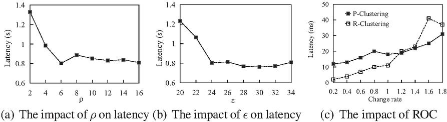
Figure 8 Varying the parameters.
In Section 4.4.1 we introduced the ROC matrix, which determines whether to perform P-clustering or R-clustering for each partition’s rate of change. When the time window size is s, we observe an average of about pivot trajectories per time window. Therefore, we take as the denominator, that is, the number of pivot trajectories in the previous time window, and randomly generate new pivot trajectories and pivot trajectories that need to be deleted to obtain different ROC. The running results are shown in Figure 8(c). As the ROC raises, the latency of both P-clustering and R-clustering increases, but P-clustering grows more slowly. When the ROC is less than , R-clustering is more efficient. Conversely, the latency of the P-clustering will be lower. Therefore we set the threshold of ROC to .
5.3 Efficiency Comparison
We evaluate the efficiency of our framework by comparing the execution time of Lunatory and CUTiS. In Figure 9, as the amount of data increases, the latency of ACTOR is always lower than that of Lunatory and CUTiS. The reason is that Lunatory re-clusters the data in each time window and does not make full use of the reusable state in the previous time window. In addition, ACTOR implements continuous trajectory clustering, using the R-tree to maintain the state of trajectories and clusters dynamically. The efficiency of search, addition, and deletion on the R-tree is higher than that of clustering from scratch, so the performance of ACTOR is higher than that of Lunatory. In order to achieve continuous clustering, CUTiS maintains the data structure of a micro-group. Micro-groups are defined based on the representative trajectories in the cluster. The mergence and split of micro-groups are also involved in each new time window, and the time complexity reaches ( represents micro-groups, represents the number of moving objects that update their sub-trajectories), so when the number of clusters in the partition and the new data are massive, the latency of CUTiS will increase suddenly.
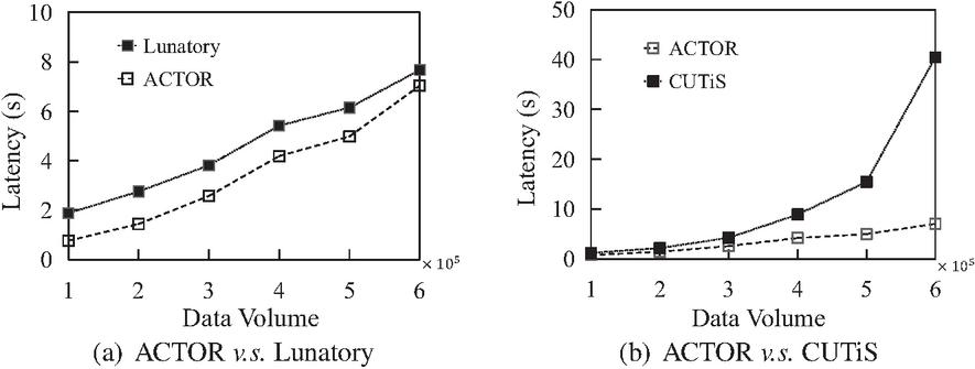
Figure 9 Execution time comparison.
Figure 10(a) depicts the memory cost of Lunatory, CUTiS, and ACTOR. Overall, Lunatory has the least memory cost because it does not require additional data structures to maintain the state of trajectories and clusters. When the amount of data is small, the memory cost of CUTiS and ACTOR are similar, and as the amount of data increases, CUTiS consumes more and more memory than ACTOR. As aforementioned, when the number of clusters and new data in the partition are tremendous, the number of micro-groups that need to be maintained will increase suddenly. In ACTOR, it benefits from our appropriate dynamic maintenance strategy, and our memory consumption is within a reasonable range.
Figure 10(b) illustrates the throughput on different datasets. On both Beijing and Chengdu datasets, the throughput of ACTOR is higher than that of Lunatory and CUTiS, which shows that our framework can be competent for continuous trajectory clustering in the incremental environment.
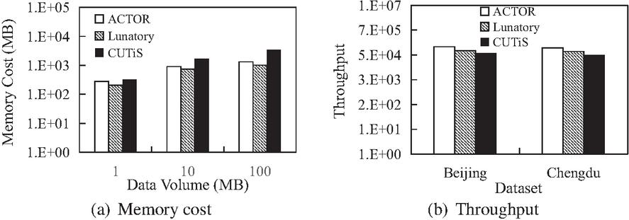
Figure 10 Memory cost and throughput comparison.
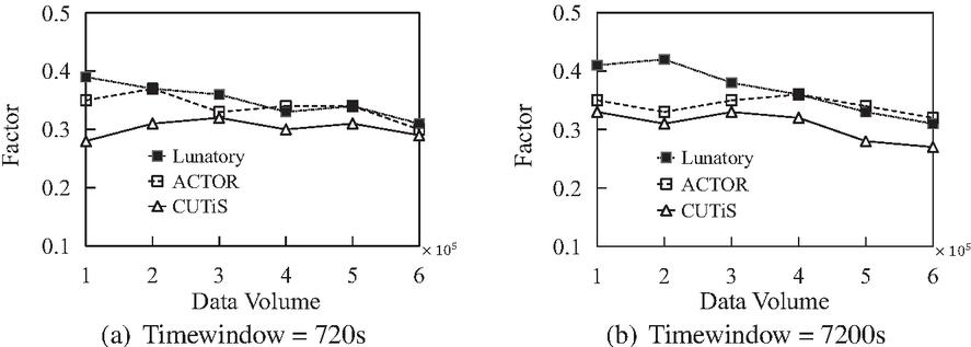
Figure 11 Clustering quality comparison.
5.4 Accuracy Comparison
The silhouette coefficient calculates the compactness of the same cluster and the interval between different clusters to judge whether the cluster is good or bad. The closer the silhouette coefficient is to , the better the clustering quality is. Figure 11 shows the silhouette coefficient values of Lunatory, CUTiS, and ACTOR in different data volumes and different time window sizes. We observe that when the window size is set to s and s, the value of the silhouette coefficient of Lunatory is higher, i.e., Lunatory’s clustering results are of better quality. The reason is that in the process of performing continuous clustering, the R-tree of maintaining clusters and trajectories inevitably produces deviations from the actual situation in the process of adding and deleting core trajectories, thus losing the quality of clustering. Nevertheless, the difference in the silhouette coefficient of ACTOR is not much different from that of Lunatory. That is, the clustering quality of the two is similar, and ACTOR also has higher execution efficiency than Lunatory.
6 Conclusion
In this paper, we propose ACTOR, an adaptive continuous trajectory clustering framework. Each trajectory is simplified into pivot trajectories with moving characteristics, then the pivot trajectories are partitioned by hexagonal-based indexing. By monitoring the ROC of each partition, the P-clustering or R-clustering is adaptively selected and executed. With the involvement of a large number of real data sets and the analysis of the experimental results, it is proved that our framework has excellent timeliness and accuracy in continuous trajectory clustering over its counterparts. We will focus our future work on the trade-off between accuracy and efficiency of distributed spatio-temporal data clustering methods. At the same time, we plan to implement an end-to-end clustering framework (from web data to analysis results).
Acknowledgements
This work was supported by National Natural Science Foundation of China under grant (No.61802273, 62102277), Postdoctoral Science Foundation of China (No.2020M681529), Natural Science Foundation of Jiangsu Province (BK20210703), China Science and Technology Plan Project of Suzhou (No.SYG202139), Postgraduate Research Practice Innovation Program of Jiangsu Province (SJCX211342).
References
[1] Pankaj K Agarwal, Kyle Fox, Kamesh Munagala, Abhinandan Nath, Jiangwei Pan, and Erin Taylor. Subtrajectory clustering: Models and algorithms. In Proceedings of the 37th ACM SIGMOD-SIGACT-SIGAI Symposium on Principles of Database Systems, pages 75–87, 2018.
[2] Mihael Ankerst, Markus M Breunig, Hans-Peter Kriegel, and Jörg Sander. Optics: Ordering points to identify the clustering structure. ACM Sigmod record, 28(2):49–60, 1999.
[3] Derya Birant and Alp Kut. St-dbscan: An algorithm for clustering spatial–temporal data. Data & knowledge engineering, 60(1):208–221, 2007.
[4] Liang Chen, Pingfu Chao, Junhua Fang, Wei Chen, Jiajie Xu, and Lei Zhao. Disatra: A real-time distributed abstract trajectory clustering. In International Conference on Web Information Systems Engineering, pages 619–635. Springer, 2021.
[5] Dorin Comaniciu and Peter Meer. Mean shift: A robust approach toward feature space analysis. IEEE Transactions on pattern analysis and machine intelligence, 24(5):603–619, 2002.
[6] Ticiana L Coelho Da Silva, Karine Zeitouni, and José AF de Macêdo. Online clustering of trajectory data stream. In 2016 17th IEEE International Conference on Mobile Data Management (MDM), volume 1, pages 112–121. IEEE, 2016.
[7] Ticiana L Coelho Da Silva, Karine Zeitouni, José AF de Macêdo, and Marco A Casanova. Cutis: optimized online clustering of trajectory data stream. In Proceedings of the 20th International Database Engineering & Applications Symposium, pages 296–301, 2016.
[8] Uber Engineering. H3: Uber’s Hexagonal Hierarchical Spatial Index. https://eng.uber.com/h3/.
[9] Martin Ester, Hans-Peter Kriegel, Jörg Sander, Xiaowei Xu, et al. A density-based algorithm for discovering clusters in large spatial databases with noise. In kdd, volume 96, pages 226–231, 1996.
[10] Ziquan Fang, Yuntao Du, Lu Chen, Yujia Hu, Yunjun Gao, and Gang Chen. E 2 dtc: An end to end deep trajectory clustering framework via self-training. In 2021 IEEE 37th International Conference on Data Engineering (ICDE), pages 696–707. IEEE, 2021.
[11] Joachim Gudmundsson and Nacho Valladares. A gpu approach to subtrajectory clustering using the fréchet distance. IEEE Transactions on Parallel and Distributed Systems, 26(4):924–937, 2014.
[12] Chih-Chieh Hung, Wen-Chih Peng, and Wang-Chien Lee. Clustering and aggregating clues of trajectories for mining trajectory patterns and routes. The VLDB Journal, 24(2):169–192, 2015.
[13] Bogyeong Kim, Kyoseung Koo, Juhun Kim, and Bongki Moon. Disc: Density-based incremental clustering by striding over streaming data. In 2021 IEEE 37th International Conference on Data Engineering (ICDE), pages 828–839. IEEE, 2021.
[14] Sirisup Laohakiat and Vera Sa-Ing. An incremental density-based clustering framework using fuzzy local clustering. Information Sciences, 547:404–426, 2021.
[15] Jae-Gil Lee, Jiawei Han, and Kyu-Young Whang. Trajectory clustering: a partition-and-group framework. In Proceedings of the 2007 ACM SIGMOD international conference on Management of data, pages 593–604, 2007.
[16] Tianyi Li, Lu Chen, Christian S Jensen, Torben Bach Pedersen, Yunjun Gao, and Jilin Hu. Evolutionary clustering of moving objects. In 2022 IEEE 38th International Conference on Data Engineering (ICDE), pages 2399–2411. IEEE, 2022.
[17] Zhenhui Li, Jae-Gil Lee, Xiaolei Li, and Jiawei Han. Incremental clustering for trajectories. In International Conference on Database Systems for Advanced Applications, pages 32–46. Springer, 2010.
[18] Jiali Mao, Qiuge Song, Cheqing Jin, Zhigang Zhang, and Aoying Zhou. Tscluwin: Trajectory stream clustering over sliding window. In International Conference on Database Systems for Advanced Applications, pages 133–148. Springer, 2016.
[19] Jiali Mao, Tao Wang, Cheqing Jin, and Aoying Zhou. Feature grouping-based outlier detection upon streaming trajectories. IEEE Transactions on Knowledge and Data Engineering, 29(12):2696–2709, 2017.
[20] Peter D Grünwald In Jae Myung and Mark A Pitt. Advances in minimum description length: Theory and applications. MIT press, 2005.
[21] Yang Wu, Zhicheng Pan, Pingfu Chao, Junhua Fang, Wei Chen, and Lei Zhao. Lunatory: A real-time distributed trajectory clustering framework for web big data. In International Conference on Web Engineering, pages 219–234. Springer, 2022.
[22] Mingxuan Yue, Yaguang Li, Haoze Yang, Ritesh Ahuja, Yao-Yi Chiang, and Cyrus Shahabi. Detect: Deep trajectory clustering for mobility-behavior analysis. In 2019 IEEE International Conference on Big Data (Big Data), pages 988–997. IEEE, 2019.
[23] Yu Zheng. Trajectory data mining: an overview. ACM Transactions on Intelligent Systems and Technology (TIST), 6(3):1–41, 2015.
Footnotes
Biographies

Yang Wu is a postgraduate student at Soochow University. His research interests mainly include trajectory data analysis and trajectory data stream clustering.

Junhua Fang is an associate professor of Soochow University. His research interests mainly include spatio-temporal database, cloud computing, and distributed stream processing.

Pingfu Chao is an associate professor of Soochow University. His research interests mainly include spatial-temporal data management, trajectory data mining, distributed database system and smart grid data analysis.

Zhicheng Pan is a Ph.D. student at East China Normal University. His research interests mainly include spatio-temporal databases and machine learning for database.

Wei Chen is an associate professor of Soochow University. His research interests mainly include spatio-temporal data analysis, knowledge graph, heterogeneous information network and data fusion.

Lei Zhao is a professor of Soochow University. His research focuses on graph databases, social media analysis, query outsourcing, parallel and distributed computing.
Journal of Web Engineering, Vol. 22_1, 105–130.
doi: 10.13052/jwe1540-9589.2216
© 2023 River Publishers