Diagnostic Classifiers for Explaining a Neural Model with Hierarchical Attention for Aspect-based Sentiment Classification

Kunal Geed¹, Flavius Frasincar¹ and Maria Mihaela Trusca^{2, 3,}*

¹Erasmus University Rotterdam, Burgemeester Oudlaan 50, 3062 PA Rotterdam, the Netherlands
²Bucharest University of Economic Studies, 010374 Bucharest, Romania
³KU Leuven, Celestijnenlaan 200A, 2402, 3001 Leuven, Belgium
E-mail: kunalgeed15@gmail.com; frasincar@ese.eur.nl; maria.trusca@csie.ase.ro
*Corresponding Author

Received 01 October 2022; Accepted 21 November 2022; Publication 14 April 2023

Abstract

The current models proposed for aspect-based sentiment classification (ABSC) are mainly developed with the purpose of providing high rates of accuracy, regardless of the inner working which is usually difficult to understand. Considering the state-of-art model LCR-Rot-hop $+, +$ for ABSC, we use diagnostic classifiers to gain insights into the encoded information of each layer. Starting from a set of various hypotheses, we test how sentiment-related information is captured by different layers of the model. Given the model architecture, information about the related words to the target is easily extracted. Also, the model is able to detect to some extent information about the sentiments of the words and, in particular, sentiments of the words related to the target. However, the model is less effective in extracting the aspect mentions associated with a word and the general structure of the sentence.

Keywords: Aspect-based sentiment classification, neural rotatory attention model, diagnostic classification.

1 Introduction

Sentiment analysis (SA) is the task that allows understanding of human opinions and preferences. Depending on the granularity level, SA applies at the document, sentence, or aspect level [17]. While SA at the document or sentence level mainly requires only a classification task, ABSC is usually executed in three steps. According to [25], the steps consist of the detection of sentiment-aspect pairs, classification of the pairs, and the aggregation of the newly obtained information. Among all these three subtasks, we focus only on the sentiment classification of aspects known as aspect-based sentiment classification (ABSC) [5].

The application of ABSC is wide, and, although more complicated than SA, can lead to a much more comprehensive analysis. For this purpose, a state-of-the-art technique was developed in [28], which proposed a hybrid approach to ABSC. Firstly, the authors make use of a domain ontology to identify aspects and sentiments towards these. Any inconclusive cases are then passed to a neural network that predicts the sentiments. Due to its high performance, we make use of this technique as the basis of our research.

Neural networks are considered to be black-box methods as the user is not able to explain the results based on the structure of the neural network, hence their inner workings are not clear. Therefore, our research aims to improve the understanding of neural networks with a focus on the architecture presented in [28], which is part of the larger field of explainable AI (XAI). To solve this problem, we investigate if the model presented in [28] can capture specific information regarding the relationships between words and aspects. We further extend this by using the domain ontology to test if LCR-Rot-hop $+, +$ can encode the domain knowledge represented, in a sentiment analysis context, in the domain ontology. To investigate these questions, we use diagnostic classifiers as introduced in [13]. The major contributions of this work are as follows. While in [19] diagnostic classifiers are used to understand the inner workings of the LCR-Rot-hop model, we focus on the more advanced LCR-Rot-hop $+, +$ model in this paper. Furthermore, in addition to diagnostic classifiers discussed in [19], we investigate if the aspects represented in the domain ontology are encoded in the neural network. To our knowledge, this is one of the first works that investigates the presence of a domain sentiment ontology signal in the representations produced by a neural attention model. All source data and code can be retrieved from https://github.com/KunalGeed/DC-LCR-Rot-hop_plus_plus.

This paper is an extension of our previous work using diagnostic classifiers for explaining LCR-Rot-hop++ [10]. To be precise, we have enlarged the related work by better stressing the differences between our solution and existing ones. Also, we have added an example for ABSC to help the reader better understand the task. More details on the explained model, LCR-Rot-hop++, are also provided. In addition, we have given information on the performance of the deep neural model that we have explained.

The paper is structured as follows. In Section 2 we discuss the literature associated with ABSC and XAI. Section 3 explores the dataset used in this study and describes the pre-processing steps used to convert the dataset into the final dataset. In Section 4, we describe the methodology of the used aspect-based sentiment classifier and the methodology of diagnostic classifiers. Section 5 presents the results. Lastly, Section 6 draws conclusions from the results, states the limitations of our study, and suggests avenues for further research.

2 Related Works

This section discusses the relevant literature for this study. Section 2.1 provides a more in-depth analysis of ABSC. Section 2.2 describes the related work of diagnostic classifiers.

2.1 Aspect-based Sentiment Classification

ABSC is the task of identifying the sentiment value of a target-sentiment pair [25] and the approaches to complete this task can be divided into three major classes, the knowledge-based approach, the machine learning approach, and the hybrid approach, which is a combination of the knowledge-based and machine learning approach.

The knowledge-based approach uses domain knowledge to perform the sub-tasks of ASBC. We discuss the ontology-based approach designed in [26]. An ontology represents the shared concepts present in a certain domain and the relationships between the concepts plus the axioms that govern the domain in a way that can be understood by machines [11]. The domain knowledge was encoded in the form of an ontology proposed in [26] for it to be understood by the computer. The ontology relies on a set of rules to identify aspects and determine the polarity of the sentiment.

More recent work on ABSC has shown good performance from machine learning approaches. ABSC is approached with a support vector machine (SVM) in [16]. They used five one-vs.-all SVM classifiers (one for each considered aspect category), and treated the task as a multi-class multi-label text classification problem to detect the aspects. For determining the polarity associated with an aspect, the authors trained linear SVM classifiers that used the information about the target term, the words around the target term, and the nodes in the parse tree connected to the target term. In [22], naive Bayes classifiers are used for the sentiment classification task for product reviews and also showed relative success. However, most success has been found in the field of deep learning, by the use of neural networks. Within neural networks, long short term memory (LSTM) [12], and its variants, have shown great success in ABSC. The left-center-right (LCR) separated neural networks are introduced in [27] for ABSC. They make use of bi-directional LSTM in their model. The purpose is to better address two problems. Firstly, how to represent the target better when the target is a phrase (multiple words) and, secondly, how to use the connection between target and context to capture the most important words to represent targets and contexts. They had further improved the model by generating new context and aspect representations adjusted by an attention mechanism applied multiple times or in a rotatory way.

Although knowledge-based approaches and machine learning approaches had shown individual success, the hybrid techniques developed by combining them proved to be of greater success. A hybrid approach to ABSC is introduced in [26], which uses an ontology-based model to first find as many sentiment classifications as possible and to pass the inconclusive cases to the bag-of-words (BOW) model, which classifies the rest. Next, the previous model is improved in [29] by changing the backup classifier to the LCR-Rot models proposed in [27]. The authors further extend and improve upon the LCR-Rot model by repeating the rotary mechanism n times (in order to refine representations), yielding the LCR-Rot-hop model. Using the methods proposed in [29] as their basis, a next set of improvements are further proposed for the LCR-Rot-hop model in [28], by introducing deep contextual word embedding and hierarchical attention leading to the LCR-Rot-hop $+, +$ model.

2.2 Diagnostic Classifiers

With the increase in the use of black-box methods, such as neural networks, there is a growing need for techniques to investigate what happens inside this black-box method part of XAI [8]. An approach similar to diagnostic classifiers was proposed in [1]. In their work, the authors outline a framework that facilitates the understanding of encoded representation using auxiliary prediction tasks. They score representations by training classifiers which take the representations as input to tackle the auxiliary prediction tasks. If the trained classifier is unable to predict the property being tested in the prediction task, then it is concluded that the representations have not encoded that information [1].

Another technique used to facilitate understanding of the models’ inner working is introduced in [2]. Using a generator model like variational auto-encoder or a generative adversarial network, the proposed approach aims to produce artificial inputs that mimic the output produced by the analyzed model. As the models are considered black-box methods with no access to their inner gradients, the optimization of the generator relies on an evolutionary strategy. In the end, the artificial inputs are analyzed to provide insights into the model capabilities.

Considering that the visualization techniques were not sufficient to gain insight into the information encoded by a recurrent neural network (RNN), diagnostic classifiers are introduced in [13] to gain better insight into the information encoded by RNNs. This led to the development of diagnostic classifiers where the authors tested multiple hypotheses about the information processed by the network. If the diagnostic classifiers can accurately predict the information, then it is concluded that the information is encoded in the network [13].

[14] makes use of diagnostic classifiers to link what is going on inside the neural network to linguistic theory. Specifically, they examine the ability of LSTM to process negative polarity items (NPIs). The results show that the model can determine a relationship between the licensing context and NPIs. As explained in [14], NPIs are words that need to be licensed by a licensing context to form a valid sentence, for example, “He did not buy any books” where “any” is an NPI and “not” is a licensing context. The authors determine that a good language model must be able to encode this relationship. This study is able successfully to link linguistic theory to deep learning [14].

The work in [3] attempts to understand the inner workings of neural networks and specifically what the neural networks learn about the target language. The authors determine that lower levels of a neural network are better at capturing morphology. Hence they also hypothesize that lower levels of the neural network capture word structure and the higher levels capture word semantics [3].

[19] makes use of diagnostic classifiers for ABSC. Specifically, the authors evaluate, in detail, the LCR-Rot-hop method developed in [29]. In [19] the LCR-Rot-hop method is analyzed to investigate if the internal layers can encode word information, such as a part-of-speech (POS) tag, sentiment value, presence of aspect relation, and aspect related sentiment value of words. The authors conclude that the word structure (POS) is captured by the lower levels of the neural network, and the higher levels are able to encode information about aspect relation and aspect related sentiment value, which is in line with a hypothesis proposed in [3],

3 Specification of the Data

This study makes use of the SemEval 2016 Dataset, Task 5, Sub-task 1, which contains an annotated dataset for ABSC [24]. Figure 1 shows an example of an annotated review found in the training dataset. A review is divided at a sentence level and for each opinion in a sentence, the target, category, and polarity are stated. The polarity of the opinion is the sentiment (positive, negative, or neutral) that the opinion has towards the target. The target is the word in the opinion towards which the sentiment is directed. Lastly, the category is related to the target and shows which aspect the target belongs to.

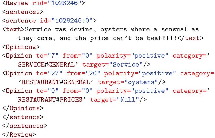
Figure 1 A sentence from the SemEval-2016 dataset.

In Figure 1, we can see that in the sentence, “Service was devine, oysters where a sensual as they come, and the price can’t be beat!!!”, the reviewer is complementing the price, food, and service of the restaurant. This is reflected in the positive polarity for each of the categories (“SERVICE#GENERAL”, “FOOD#QUALITY”, and “RESTAURANT#PRICES”) and associated targets expressed in the sentence.

Table 1 shows the class frequencies for the training and test set used to evaluate LCR-Rot-hop $+, +$ . In both the test and training set, the positive class is in the majority with more than 70%, and the neutral class is in the minority with less than 5%. This imbalance could make it more difficult for the neural network to learn the neutral class.

Table 1 Polarity frequencies in training and test sets

Training Data			Test data
Polarity	Frequency	%	Polarity	Frequency	%
Negative	488	26.0	Negative	135	20.8
Neutral	72	3.8	Neutral	32	4.9
Positive	1319	70.2	Positive	483	74.3

Due to the fact that we use BERT word embedding to represent words, we need to re-concatenate words that have been divided into word pieces in order to generate the dataset used to train and test the diagnostic classifiers. As any words that begin with “##” is a word piece belonging to the word preceding it, we can combine them into a single word. Due to each word also needing its own BERT word piece embedding and hidden states, when we combine the word pieces we also need to generate a single word embedding or hidden states for the newly formed word. The word embedding and hidden states represent the layer information that is output by each layer of the LCR-Rot-hop $+, +$ model, prior to the final MLP layer for sentiment classification. A proposed solution [31] was to use a recurrent neural network to combine word piece embeddings into a single word embedding, however, without a large dataset to train the neural network this would result in inadequate word embeddings. One of the methods to get a single embedding that captures the meaning of a larger piece of text, such as a phrase or a sentence, from the individual embedding is to average the word embedding to get a single word embedding representing the entire phrase [15]. We use this approach to combine word pieces and their embeddings and layer information into a single vector due to its simplicity.

4 Method

This section is dedicated to the proposed methodology. Section 4.1 presents the backup model of the the two-step approach HAABSA $+, +$ , and Section 4.2 provides an overview of the diagnostic classifiers used to understand the inner working of the LCR-Rot-hop $+, +$ model.

4.1 LCR-Rot-hop $+, +$

In this study we make use of the LCR-Rot-hop $+, +$ model proposed by [28]. This model is specifically designed for the task of target sentiment classification. LCR-Rot-hop $+, +$ model makes use of the LCR-Rot model proposed by [27] as its basis. Other approaches tend to not account for the size of the target, as it can range from being a single word to phrase [27]. We begin by splitting the sentence into three parts, the left context, the target, and the right context. The word embeddings, BERT in this case, are also generated for the words in the sentence.

We make use of BERT embeddings in this study as the research by [28] showed that BERT embeddings led to best performance for the HAABSA $+, +$ model. BERT embeddings are contextual word embeddings which take into account the context surrounding the words when coming up with vector representation of the words [9]. Hence the same word can have different BERT embeddings as it is likely to have different contexts. To this end, when generating the embeddings we follow the same procedure as [28]. The words are labeled using a coding number to differentiate between multiple occurrences of the same word. For this study we used the BERT embedding generated by [28] as we make use of the same dataset. Furthermore the length of the BERT embedding vector was set to be 768 by [28], which we follow also in our study.

Now we describe the LCR-Rot-hop $+, +$ model method-4 proposed by [28]. The left, target and right context are fed into three bi-directional long short term memory (LSTM) cells which output hidden states $[h_{1}^{l}, h_{2}^{l}, \dots, h_{L}^{l}]$ , where $L$ is the number of words in the left context, $[h_{1}^{r}, h_{2}^{r}, \dots, h_{R}^{r}]$ , where $R$ is the number of words in the right context, and $[h_{1}^{t}, h_{2}^{t}, \dots, h_{T}^{t}]$ , where $T$ is the number of words in the target. After this a two-step rotatory attention mechanism is applied on the hidden states. Below we describe the two-step rotatory attention mechanism. The formulas are symmetrical for left and right side, hence we show it only for one side.

Step 1: We use an average pooling operation to get the vector $r^{t_{p}}$ . We also use $r^{t_{p}}$ and the hidden states extracted from the left context to generate the attention scores. The attention scores are given in Equation (1). $W_{c}^{l}$ is the weight matrix and $b_{c}^{l}$ is the bias term.

f (h_{i}^{l}, r^{t_{p}}) = \tanh (h_{i}^{l} \times W_{c}^{l} \times r^{t_{p}} + b_{c}^{l}) .

(1)

Using a softmax function, a normalized attention scores are calculated which take $f (h_{i}^{l}, r^{t_{p}})$ as input.

α_{i}^{l} = \frac{\exp (f (h_{i}^{l}, r^{t_{p}}))}{\sum_{j = 1}^{L} \exp (f (h_{j}^{l}, r^{t_{p}}))} .

(2)

Using the left normalized attention scores and the hidden states of the left context we generate the left context representation. This is the left target2context vector and is shown in Equation (3). The right target2context is generated in a similar fashion using the hidden states from the right context.

r^{l} = \sum_{i = 1}^{L} α_{i}^{l} \times h_{i}^{l} .

(3)

Step 2: In this step we generate the target representation. The target representation is divided into two parts, the left target representation and the right target representation. These representations make use of the left and right context representations calculated in Step 1. The attention scores are computed as shown in Equation (4).

f (h_{i}^{t}, r^{l}) = t a n h (h_{i}^{t} \times W_{c}^{t} \times r^{l} + b_{c}^{t})

(4)

Then we calculate the normalized attention score similar to in Step 1 as shown in Equation (5).

α_{i}^{t_{l}} = \frac{\exp (f (h_{i}^{t}, r^{l}))}{\sum_{j = 1}^{T} \exp (f (h_{j}^{t}, r^{l}))} .

(5)

Lastly, we use the normalized attention scores to calculate the left context-aware target representation depicted in Equation (6).

r^{t_{l}} = \sum_{i = 1}^{T} α_{i}^{t_{l}} \times h_{i}^{t} .

(6)

This model was improved by [29] by repeating Step 1 and Step 2 $n$ number of times (hops). After the first iteration, in Step 1 the $r^{t_{p}}$ is replaced by the left ( $r^{t_{l}}$ ) or right ( $r^{t_{r}}$ ) context-aware representation depending on the side. The ideal number of hops was found to be three hops [29]. [28] furthered this method by implementing hierarchical attention into the model. Before, the model only make use of local information, but by including hierarchical attention one can update the target2context and context2target vector using a relevance score calculated at the sentence level [28]. The authors found that the neural network gave the best performance when the hierarchical attention was applied to all hops of the rotatory attention mechanism. The process for applying hierarchical attention to the context2target and target2context vector is shown below. Firstly, the attention function $f (v_{i})$ is calculated, where $v_{i} \in r^{l}, r^{r}, r^{t_{l}}, r^{t_{r}}$ and $W$ is the weight matrix and $b$ is the bias term.

f (v_{i}) = \tanh (V_{i} \times W + b) .

(7)

We use the attention function to calculate the normalized attention scores for each context. [28] normalizes the score for the left and right context representations together and the left target and right target representations together. Hence we have the following conditions, $α_{1} + α_{4} = 1$ and $α_{2} + α_{3} = 1$ , $α_{1}$ is the left normalized attention score, $α_{2}$ is the left target normalized attention score, $α_{3}$ is the right target normalized attention score and $α_{4}$ is the right normalized attention score. Equation (8) shows the calculation for the left and right normalized attention score. The normalized attention scores for the left-target and right-target are calculated in a similar manner.

α_{i} = \frac{\exp (f (v^{i}))}{\sum_{j \in 1, 4} \exp (f (v^{j}))} .

(8)

Finally the context2target and target2context are scaled using their respective attention scores.

v^{i^{'}} = α_{i} \times v^{i} .

(9)

After applying hierarchical information over multiple hops, we have the four context representations: left context representation, right context representation, and the target representations from the left and right context point of view. These are concatenated and fed into a MLP with softmax function designed for sentiment classification. The whole neural network architecture is showcased in Figure 2.

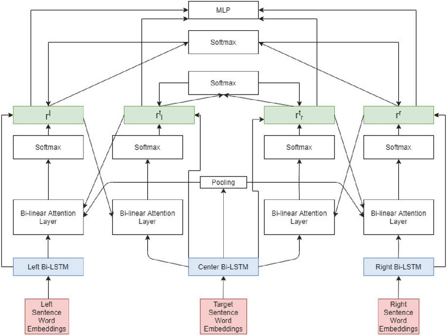
Figure 2 Architecture of LCR-Rot-hop $+, +$ .

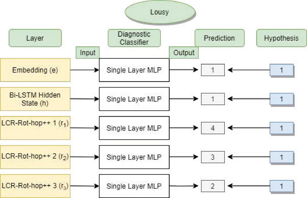
Figure 3 Overview of the diagnostic classifier.

4.2 Diagnostic Classifier

An overview of diagnostic classifiers is provided in Figure 3. In this figure, we are evaluating the word “lousy” for the POS hypothesis. Knowing that each word is assigned a label that ranges between 0 and 4 for POS tags: nouns, adjectives, adverbs, verbs, or “remaining” words, we notice that the adjective “lousy” is properly classified only by the first layers of the model.

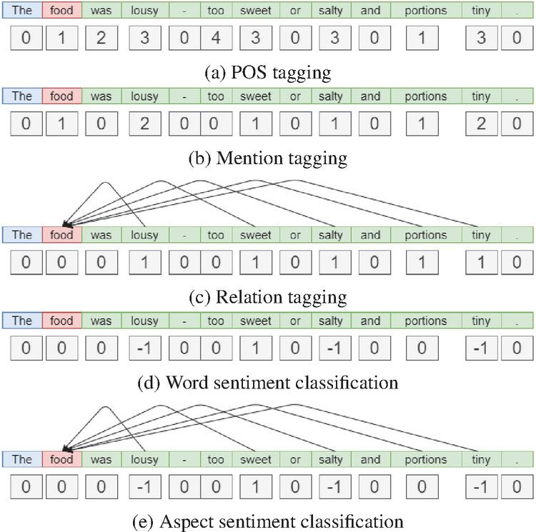
Figure 4 Examples with POS tagging, mention tagging, relation tagging, word sentiment classification, and aspect sentiment classification.

In this paper, we test various hypotheses to analyze whether the neural network encodes certain information. Below we list the various hypotheses being tested in this paper and how the corresponding tests are generated. Some of these have already been considered in [19]; however, for the simpler LCR-Rot-hop model and not the advanced LCR-Rot-hop $+, +$ model.

POS tagging is the process of assigning tags to the words based on their POS and their grammatical categories such as tense, singular/plural, etc. Due to limited amounts of data available we omit POS tags, already mentioned above. The words classified as anything other than these four are categorized under “remaining”. This process is done using the Stanford CoreNLP package [18]. The POS hypothesis is designed to check if the neural network can understand the structure of a sentence and its various components. Figure 4a shows an example for POS classification.

Mention tagging involves predicting the aspect mention related to the word. We use the ontology to identify the aspect mention a word is connected to. We match the word to a concept in the ontology and ensure maximum matches by checking all lexicalizations of a concept. If there is a match, we check what aspect mention this concept is a subclass of in order to identify the aspect the word is referring to. Due to the limited coverage of the ontology, the size of this dataset is much more limited than the others. The mention tagging hypothesis helps to understand what part of the ontology the neural network can understand and is encoded in the neural network. We test the mention tagging hypothesis by checking if the neural network can identify various aspects of the ontology. An example of mention tagging is given in Figure 4b.

Aspect relation classification is the task of predicting the presence of a relation between the words in the context and the target/aspect. Hence, this is a binary classification problem. To generate the dataset, we make use of the Stanford Dependency Parser [7], which identifies the various grammatical relationships between words in a sentence. If any relationships exist between a context word and its target, we label that word as 1, and 0, otherwise. The aspect relation hypothesis helps to check if the neural network is encoding information about the relationship between a context word and the target. Figure 4c shows an example of relation tagging. The dependencies are indicated by an arrow from the context word to the target word.

Word sentiment classification is the task of predicting the sentiment of a word as either positive, neutral/no sentiment, or negative. To identify word sentiment, we make use of a two-step procedure. First, we match the word to a concept in the ontology if it is possible. For this, we use the various lexical representations a concept has. After matching words to a concept, we check if the concept belongs to the positive or negative subclasses of the sentiment value class defined in the ontology and use that to identify the sentiment. If the word does not match any concept in the ontology or is related to a concept that does not belong to the positive or negative subclasses, we use as back-up the NLTK SentiWordNet library [4] to identify the word sentiment. NLTK SentiWordNet identifies the sentiment based on its most frequently used context. It can also classify the word as neutral/no sentiment. Due to the limited coverage of the ontology, we have to use the NLTK SentiWordNet so that we have a larger dataset to be used to train and test. The word sentiment hypothesis is designed to identify if the neural network can correctly detect the sentiment of the word. Figure 4d shows an example of word sentiment classification.

Target-related sentiment classification is a combination of the previous two tasks discussed, namely word sentiment classification and aspect relation classification. We generate another dataset which combines the information from the previous two datasets. If a word has a relation with the target (aspect relation classification) we gather the sentiment of the word (word sentiment classification) and assign that sentiment. If there is no relation or if the sentiment is neutral, we identify it as “no sentiment”. The target-related sentiment hypothesis checks if the neural network can identify the words that have a relation to the target and what sentiment they hold. An example of this can be seen in Figure 4e.

The diagnostic classifiers are implemented using the scikit-learn library in Python. We make use of the MLPClassifier function in the library for the diagnostic classifiers. MLPClassifer has the ReLU activation function and a constant learning rate of 0.001. Hyper-parameter optimization was performed using the GridSearchCV function provided in the scikit-learn library on the training data with three folds. Due to time and computational constraints we only optimize the number of neurons in the neural network for each of the diagnostic classifiers. We vary the number of neurons from 500 to 1100 with increments of 200.

5 Evaluation

This section discusses and presents the results of this study. Section 5.1 discusses the evaluation measures used to gauge the performance of the diagnostic classifiers. Section 5.2 discuss the performance of the LCR-Rot-hop $+, +$ model. Section 5.3 presents the results for the diagnostic classifiers. Section 5.4 summarizes our findings with respect to the tested hypotheses.

5.1 Evaluation Measures

To measure the performance of any classifiers, there exist different performance measures. For this study, we limit ourselves to the weighted F1 score and the accuracy as performance metrics. Both of these measures are implemented using the scikit-learn library on Python. Accuracy measures the closeness between between predicted and true class label of data instances [20]. A higher accuracy would indicate a better model; however, it is not the case when the dataset is imbalanced because the minority classes have a small impact on the accuracy compared to the majority class [30]. Hence, the accuracy measures could possibly lead to incorrect conclusions when evaluating results and checking what the neural network is learning best out of all the hypotheses. To this end, we also include the weighted F1 measure as a performance measure in our dataset, which calculates a F1 score accounted for class imbalance [23]. The F1 measure is more robust to imbalances, as it is the harmonic mean between the recall and precision, hence a higher F1 measure indicates higher performance [30]. Hence, a weighted F1 measure is likely to give a more accurate depiction of the learning capabilities of the diagnostic classifiers and through them the original neural network.

5.2 LCR-Rot-hop $+, +$ Model

In [28], it is determined that the best results, an accuracy of 87.0%, for the neural network model, were found using BERT embeddings as input and applying hierarchical attention at all the hops. The authors had also compared BERT to non-contextual word embeddings such as GloVe which was used in [29] and contextual word embeddings such as ELMo. The HAABSA $+, +$ model was compared to other state-of-the-art models for ABSC and the winners of the SemEval 2015 and 2016 contests. The authors found that HAABSA $+, +$ performance tied with the winning method of the SemEval 2015 contest and came second in the SemEval 2016 contest. This study only focuses on the LCR-Rot-hop $+, +$ model and not the complete hybrid method. Hence, only the neural network was replicated for the sake of this research.

The results are shown in Table 2. We observe an overall accuracy of 86.6% for the test set and 90.6% for the training set. This result does suggest that there might be slight overfitting, as the observed training accuracy is higher than the test accuracy. If we further break down the accuracy in the training set and test set, we notice that the accuracy for the neutral class is extremely low, which is expected due it being the minority class which accounts for only 3.8% of the total training data. This is due to the fact the LCR-Rot-hop $+, +$ model did not have enough instances of the neutral class to train on. Lastly, the positive class is the majority class and it can be seen that the neural network excels at identifying positive instances. Our overall results were slightly different from the ones reported in [28].

A possible reason could be due to the difference in hyper-parameter for the neural networks and the fact that the model has a certain degree of randomness due to it selecting random batches to train the network. Furthermore, the results were reported for the hybrid model, which included the use of an ontology. It is possible that the ontology was able to identify difficult instances and only pass easier ones to the neural network, resulting in higher overall accuracy.

Table 2 Results for the LCR-Rot-hop $+, +$ model

	Training Set		Test Set
	Size %	Accuracy %	Size %	Accuracy %
Negative	26.0	89.37	20.8	82.96
Neutral	3.8	1.4	4.9	0
Positive	70.2	95.91	74.3	93.38
Total	100	90.63	100	86.61

Table 3 Diagnostic classifier results for POS tagging

Layer	Accuracy (%)	F1 (%)	Number of Neurons
Embedding	65.51	69.96	500
Hidden state	58.18	63.58	700
Hierarchical weighted state 1	55.57	61.53	500
Hierarchical weighted state 2	55.54	61.62	500
Hierarchical weighted state 3	56.50	62.19	700

The whole model is implemented in Python 3.5. We make use of the TensorFlow 1.13 library to develop the models and use the model developed in [28] as the basis for our code. For the ontology we make use of the Owlready2 library, which is designed to create and explore ontologies.

5.3 Diagnostic Classifier

This subsection is dedicated to the analysis of the diagnostic classifiers. The subsection is structured as follows. Sections 5.3.1 and 5.3.2 are related to the POS tagging and aspect mention hypotheses, respectively. The next three sections, 5.3.3, 5.3.4, and 5.3.5, are dedicated to the classification of the aspect relations, word sentiments and target-related sentiments, respectively.

5.3.1 POS tagging

Table 3 shows the results for the diagnostic classifier trained to predict the POS tag of a word. Table 3 shows that the accuracy is highest for the embedding layer but falls as we move deeper into the neural network, although there is a slight increase at the end. A similar trend is shown by the F1 score, although there is an increase in the weighted F1 score in the second weighted hierarchical layer. This suggests that the deeper layers of the neural network encode less information about the POS tags. Overall, the embedding layer tends to best encode information about the structure of the sentence, while the information is lost or becomes less pronounced in the data as it moves deeper into the network. According to the results reported in [19], a steep fall in the accuracy is visible after the embedding layer, which continues in the hidden state layer. Last, the accuracy is stabilized for the weighted layers, although there is a slight increase in the third weighted layer, which is also observed in our results. However, our reported accuracies for POS tags are significantly lower compared to [19]. A possible reason for the relatively low accuracy and F1 scores could be the BERT embeddings used to represent words. This could confuse the diagnostic classifier as the same words have different representations, in different contexts, but could still have the same POS tag. As we move deeper into the neural network, we are losing information regarding the POS tags which suggest that the model is deeming it unnecessary for sentiment classification. The optimal number of neurons for each classifier is given in Table 3.

5.3.2 Aspect mention tagging

Aspect mention tagging is a new task introduced in the current work to check if the various aspects in the domain are being encoded in the neural network. According to Table 4, the accuracy falls as we move deeper into the model. While the BERT embedding layer has the highest accuracy, the hierarchical weighted layers are the least effective. However, within the hierarchical weighted layers, the accuracy only decreases minutely and is relatively stable. It is to be noted that the mention tagging hypothesis has a highly imbalanced dataset, and after balancing the dataset we are left with a much smaller dataset which might adversely affect the classifier. Furthermore, due to the imbalance in the data, the weighted F1 is a better evaluation metric and also provides a slightly different result. According to F1, the performances of the embedding layer and the hidden state are extremely close to each other. The embedding layer is below the hidden layer by an extremely small margin. The trend for the weighted F1 scores is downwards, similar to the accuracy. From this information, we can see that the embedding layer is able to best encode information about the aspect mentions. Overall, our results suggest that as we move deeper into the neural network, information about the aspects is to some extent lost. It is to be noted that a word could be related to multiple aspects, and hence a multi-class diagnostic classifier could be replaced with a multi-label diagnostic classifier. The optimal number of neurons for each classifier is given in Table 4.

Table 4 Diagnostic classifier results for mention tagging

Layer	Accuracy (%)	F1 (%)	Number of Neurons
Embedding	79.50	61.91	500
Hidden state	77.08	61.99	900
Hierarchical weighted state 1	73.49	60.40	700
Hierarchical weighted state 2	73.37	59.68	500
Hierarchical weighted state 3	73.15	58.22	500

5.3.3 Aspect relation classification

Table 5 shows the results of the diagnostic classifier for identifying aspect relations. This task checks if the neural network can identify words that are related to the target. Table 5 shows that the highest accuracy is present in the hidden state layer, while the lowest accuracy is in the embedding layer. As we go deeper into the neural network we see a huge spike in its ability to encode aspect relations at the hidden states layers, but after that, there is a small decline in accuracy for the next layer followed by small fluctuations in the remaining layers. A similar pattern is seen in the weighted F1 score, where the hidden state layer can encode the aspect relations best. This suggests that the model can identify words related to the target better as we move deeper into the neural network and although there is a small drop moving into the hierarchical layers, the model is able to identify words related to the target relatively well. This is logical as the neural network aims to identify words that are related to the target, towards which it is trying to classify the sentiment, and hence its ability to identify words related to the target should improve as we go deeper into the model. Out of all the layers, the hidden states appear to encode aspect relations the best. A possible reason for the hidden state performing better than the hierarchical layers could be that some words are related to the aspect but have no sentiment value, hence the model does not pay attention to those kinds of words deeper into the model, resulting in slightly lower accuracy. [19] showcases a similar pattern for aspect relations. There is a spike for the hidden state layer followed approximately the same values (or lower) for the weighted layers. The optimal number of neurons for each classifier is given in Table 5.

5.3.4 Word sentiment classification

Table 6 shows the performance of the diagnostic classifiers for identifying the sentiment of a word. The results prove that as we go deeper into the neural network, the accuracy and the weighted F1 score fall, although there is a spike for the third hierarchical weighted layer. A possible reason for the higher performance of the BERT embedding layer is probably due to the nature of word embeddings that can hold information about their context, alleviating the problem of sentiment detection. Overall, we see that information about the word sentiments is lost as we move deeper into the network. This could be justified due to type-2 sentiment mentions [28] causing some words to not be important for determining the sentiment towards the target as they are not related to that aspect. [19] does find a similar downward trend initially, although at a much higher accuracy. [19] observes that following the downward trend, the accuracy stabilizes for the weighted layers, however this is not the case for this study as we observe another increase in the final layer. The optimal number of neurons for each classifier is given in Table 6.

Table 5 Diagnostic classifier results for aspect relations

Layer	Accuracy (%)	F1 (%)	Number of neurons
Embedding	73.06	78.03	700
Hidden state	82.38	84.04	900
Hierarchical weighted state 1	80.85	82.79	500
Hierarchical weighted state 2	81.89	83.53	1100
Hierarchical weighted state 3	80.66	82.58	900

Table 6 Diagnostic classifier results for word sentiment

Layer	Accuracy (%)	F1 (%)	Number of neurons
Embedding	77.03	80.81	900
Hidden state	67.84	73.69	900
Hierarchical weighted state 1	66.82	72.95	700
Hierarchical weighted state 2	63.13	70.27	1100
Hierarchical weighted state 3	66.00	72.01	900

5.3.5 Target-related sentiment classification

Table 7 shows the results for the diagnostic classification of the target-related sentiment classification task, which has to check if the neural network can predict the sentiment of the words specifically related to the target. Table 7 shows that the accuracy is highest in the hidden state layer and falls as we move deeper into the neural network, before rising again in the final layer. However, the accuracy never increases past the hidden state layer. The weighted F1 score follows a similar pattern, although it is much less pronounced for the spike in the final layer. As the target-related sentiment hypothesis is a combination of two other hypotheses, its trend can be explained through them. We observe that the aspect relation accuracy increases and then stabilizes, but for the word sentiment hypothesis it decreases before a spike in accuracy at the end. The increase in accuracy for the hidden state layer is possibly due to the increase in the layers’ ability to identify words related to the target being greater than the fall in its ability to identify the sentiment. Furthermore, as the accuracy for sspect relations stabilizes, but the accuracy for the word sentiment hypothesis continues to fall, we observe a downward trend for the layers following the hidden state. However, the final spike can be explained by the spike in accuracy for the word sentiment hypothesis, while the accuracy of the aspect relation hypothesis remains approximately the same. We observe that the neural network places more importance on identifying the sentiment of the words related to the aspect, as we observe a relatively good accuracy for target-related sentiment classification in the final layer, which is within expectations as that is an important task for ABSC. The optimal number of neurons for each classifier is given in Table 7.

Table 7 Diagnostic classifier results for target-related word sentiment

Layer	Accuracy (%)	F1 (%)	Number of neurons
Embedding	76.88	85.27	500
Hidden state	78.05	87.22	700
Hierarchical weighted state 1	76.05	85.58	700
Hierarchical weighted state 2	75.38	85.10	1100
Hierarchical weighted state 3	77.28	85.61	500

5.4 Findings with respect to hypotheses

Figures 5a and 5b show the accuracy and F1 scores, respectively, for the different hypotheses in a single graph. We can see in Figure 5b that the model is successful at learning about aspect relations, word sentiments, and the sentiment of the word if it is related to the target (target-related word sentiment). This is a good sign as these tasks are extremely important for ABSC. A major difference between Figures 5a and 5b is that the mention tagging hypothesis performs the worst when compared using the weighted F1 score but good when comparing based on the accuracy. A reason for this disparity in results could be due to the data imbalance and the fact that the mention tagging dataset is much smaller compared to the other hypotheses datasets due to the limited coverage of the ontology. The performance for POS tagging and mention tagging is low, based on the weighted F1 score, which suggests that the model is not able to encode information about the structure of the sentence and which aspect mention a word is related to. These results are to be expected as these tasks are not important for ABSC, as identifying the sentiment supersedes POS tagging and the aspect mentions are usually already identified.

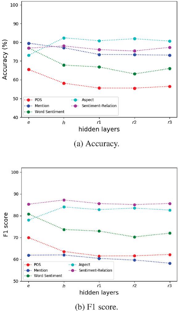
Figure 5 Overview of the accuracy and F1 score for the different hypotheses.

From these results, we can conclude that while the LCR-Rot-hop $+, +$ model learns about the word sentiment and structure of the sentence in the starting layers, the more complex details such as which words are related to the target and the sentiment of those words are learnt deeper into the model.

6 Conclusion

This study aims to gain insight into the inner working of the LCR-Rot-hop $+, +$ model and to understand whether it can capture sentiment-related information. Our findings are listed below:

• POS tagging: We noticed that the BERT embeddings were the best at classifying POS tags, while the other layers had significantly lower accuracy and F1 scores. This implied that deeper into the model, information about the POS tags is not encoded. According to the weighted F1 score, the LCR-Rot-hop $+, +$ model does not capture information about the structure of the sentence.

• Mention tagging: We found that the accuracy and weighted F1 score significantly fell as we go deeper into the model. This implied that the neural network did not encode information about the aspect mention related to the word. The best accuracy for mention tagging was found in the embedding layer. This also suggested that the model did not find this information important as we lose this information as we proceed deeper into the network.

• Aspect relation: The neural network was able to encode information regarding which words are related to the target. We found relatively high accuracy and weighted F1 score. The weighted F1 score and the accuracy rose into deeper layers of the network and stabilized at the hierarchical weighted layers. This means that the network was able to learn information about which words are related to the targets.

• Word sentiment: The ability to identify the sentiment of a word fell as we went deeper into the neural network. The best accuracy and weighted F1 score were found for the embedding layer. The relatively high accuracy and weighted F1 score for the embedding layer could be due to the contextualization. Overall, the LCR-Rot-hop $+, +$ showed moderate success in encoding information regarding the word sentiments.

• Target-related word sentiment: We found that the hidden state layer had the highest accuracy for the ability to identify words that are related to the target and then their sentiment. As we moved deeper to the network it fell for a bit before once again rising. Overall, we found that the neural network is able to encode information regarding the sentiments of the words related to the target the best, which was expected as this information is highly relevant for ABSC.

In the future, this research should be repeated for different neural networks designed for ABSC, as that might give insight into what kind of neural networks work best for certain hypotheses. Furthermore, for the mention tagging hypothesis, a multi-class, multi-label diagnostic classifier could be trained to account for one word being related to multiple aspect mentions. In addition, as imbalanced datasets are present in the real world, we should look to combine the model with more advanced re-sampling techniques, such as condensed nearest neighbor [21]. It is to be noted that this procedure must be done carefully, as certain oversampling techniques, such as SMOTE [6] and its variants, generate synthetic data and adding synthetic data is counter-intuitive as we want to investigate if the hypothesis is encoded in the layers originally. Another suggestion would be to explore how and where the neural network learns other concepts represented in the ontology besides the aspect mention (e.g., sentiment expressions). Last, we would like to refine the word sentiment by first defining a word sense disambiguation procedure and then looking after the corresponding sentiment in the ontology SentiWordNet.

References

[1] Y. Adi, E. Kermany, Y. Belinkov, O. Lavi, and Y. Goldberg. Fine-grained analysis of sentence embeddings using auxiliary prediction tasks. In 2017 International Conference on Learning Representations (ICLR 2017), 2016.

[2] A. Barbalau, A. Cosma, R. T. Ionescu, and M. Popescu. A generic and model-agnostic exemplar synthetization framework for explainable AI. In 31st European Conference on Machine Learning and Principles and Practice of Knowledge Discovery in Databases (ECML-PKDD 2020), volume 12458 of LNCS, pages 190–205. Springer, 2020.

[3] Y. Belinkov, N. Durrani, F. Dalvi, H. Sajjad, and J. R. Glass. What do neural machine translation models learn about morphology? In 55th Annual Meeting of the Association for Computational Linguistics (ACL 2017), pages 861–872. ACL, 2017.

[4] S. Bird, E. Klein, and E. Loper. Natural Language Processing with Python, Analyzing Text with the Natural Language Toolkit, volume 44. O’Reilly, 2010.

[5] G. Brauwers and F. Frasincar. A survey on aspect-based sentiment classification. ACM Computing Surveys, 2021.

[6] N. Chawla, K. Bowyer, L. Hall, and W. Kegelmeyer. SMOTE: Synthetic minority over-sampling technique. Journal of Artificial Intelligence Research, 16:321–357, 2002.

[7] D. Chen and C. D. Manning. A fast and accurate dependency parser using neural networks. In 2014 Conference on Empirical Methods in Natural Language Processing (EMNLP 2014), pages 740–750. ACL, 2014.

[8] G. Chrupała and A. Alishahi. Correlating neural and symbolic representations of language. In 57th Annual Meeting of the Association for Computational Linguistics (ACL 2019), pages 2952–2962. ACL, 2019.

[9] J. Devlin, M.-W. Chang, K. Lee, and K. Toutanova. BERT: Pre-training of deep bidirectional transformers for language understanding. In 2009 Conference of the North American Chapter of the Association of Computational Linguistics: Human Language Techniques (NAACL-HLT 2019), pages 4171–4186, 2019.

[10] K. Geed, F. Frasincar, and M. M. Truşcǎ. Explaining a deep neural model with hierarchical attention for aspect-based sentiment classification using diagnostic classifiers. In 22nd International Conference on Web Engineering (ICWE 2022), volume 13362 of LNCS, pages 268–282. Springer, 2022.

[11] S. Grimm, A. Abecker, J. Völker, and R. Studer. Ontologies and the Semantic Web, pages 507–579. 2011.

[12] S. Hochreiter and J. Schmidhuber. Long short-term memory. Neural Computation, 9(8):1735–1780, 1997.

[13] D. Hupkes and W. Zuidema. Visualisation and ‘diagnostic classifiers’ reveal how recurrent and recursive neural networks process hierarchical structure (extended abstract). In 27th International Joint Conference on Artificial Intelligence (IJCAI 2018), pages 5617–5621. International Joint Conferences on Artificial Intelligence Organization, 2018.

[14] J. Jumelet and D. Hupkes. Do language models understand anything? On the ability of LSTMs to understand negative polarity items. In 2018 EMNLP Workshop: Analyzing and Interpreting Neural Networks for NLP (BlackBox NLP 2019), pages 222–231. ACL, 2018.

[15] T. Kenter and M. de Rijke. Short text similarity with word embeddings. In 24th ACM International on Conference on Information and Knowledge Management (CIKM 2015), pages 1411–1420. ACM, 2015.

[16] S. Kiritchenko, X. Zhu, C. Cherry, and S. Mohammad. NRC-Canada-2014: Detecting aspects and sentiment in customer reviews. In 8th International Workshop on Semantic Evaluation (SemEval 2014), pages 437–442. ACL, 2014.

[17] B. Liu. Sentiment Analysis: Mining Opinions, Sentiments, and Emotions. Cambridge University Press, 2 edition, 2020.

[18] C. D. Manning, M. Surdeanu, J. Bauer, J. R. Finkel, S. Bethard, and D. McClosky. The stanford CoreNLP natural language processing toolkit. In 52nd Annual Meeting of the Association for Computational Linguistics (ACL 2014), pages 55–60. ACL, 2014.

[19] L. Meijer, F. Frasincar, and M. M. Truşcă. Explaining a neural attention model for aspect-based sentiment classification using diagnostic classification. In 36th Annual ACM Symposium on Applied Computing, SAC 2021, pages 821–827. ACM, 2021.

[20] A. Menditto, M. Patriarca, and B. Magnusson. Understanding the meaning of accuracy, trueness and precision. Accreditation and Quality Assurance, 12:45–47, 2007.

[21] A. More. Survey of resampling techniques for improving classification performance in unbalanced datasets. arXiv preprint arXiv:1608.06048.

[22] M. S. Mubarok, K. Adiwijaya, and M. D. Aldhi. Aspect-based sentiment analysis to review products using naïve bayes. In AIP Conference Proceedings, volume 1867, page 020060. AIP Publishing, 2017.

[23] F. Pedregosa, G. Varoquaux, A. Gramfort, V. Michel, B. Thirion, O. Grisel, M. Blondel, P. Prettenhofer, R. Weiss, V. Dubourg, J. Vanderplas, A. Passos, D. Cournapeau, M. Brucher, M. Perrot, and E. Duchesnay. Scikit-learn: Machine learning in Python. Journal of Machine Learning Research, 12:2825–2830, 2011.

[24] M. Pontiki, D. Galanis, H. Papageorgiou, I. Androutsopoulos, S. Manandhar, M. AL-Smadi, M. Al-Ayyoub, Y. Zhao, B. Qin, O. De Clercq, V. Hoste, M. Apidianaki, X. Tannier, N. Loukachevitch, E. Kotelnikov, N. Bel, S. M. Jiménez-Zafra, and G. Eryiğit. SemEval-2016 task 5: Aspect based sentiment analysis. In 10th International Workshop on Semantic Evaluation (SemEval 2016), pages 19–30. ACL, 2016.

[25] K. Schouten and F. Frasincar. Survey on aspect-level sentiment analysis. IEEE Transactions on Knowledge and Data Engineering, 28(3):813–830, 2016.

[26] K. Schouten and F. Frasincar. Ontology-driven sentiment analysis of product and service aspects. In 15th Extended Semantic Web Conference (ESWC 2018), volume 10843 of LNCS, pages 608–623. Springer, 2018.

[27] Z. Shiliang and R. Xia. Left-center-right separated neural network for aspect-based sentiment analysis with rotatory attention. arXiv preprint arXiv:1802.00892, 2018.

[28] M. M. Truşcǎ, D. Wassenberg, F. Frasincar, and R. Dekker. A hybrid approach for aspect-based sentiment analysis using deep contextual word embeddings and hierarchical attention. In 20th International Conference on Web Engineering (ICWE 2020), volume 12128 of LNCS, pages 365–380. Springer, 2020.

[29] O. Wallaart and F. Frasincar. A hybrid approach for aspect-based sentiment analysis using a lexicalized domain ontology and attentional neural models. In 16th Extended Semantic Web Conference (ESWC 2019), volume 11503 of LNCS, pages 363–378. Springer, 2019.

[30] S. Yanmin, A. Wong, and M. S. Kamel. Classification of imbalanced data: A review. International Journal of Pattern Recognition and Artificial Intelligence, 23, 2011.

[31] Z. Zhang, Y. Wu, H. Zhao, Z. Li, S. Zhang, X. Zhou, and X. Zhou. Semantics-aware BERT for language understanding. In 34th AAAI Conference on Artificial Intelligence (AAAI 2021), pages 687–719. AAAI Press, 2020.

Biographies

Kunal Geed is an M.Sc. student in data science and AI at Eindhoven University of Technology, the Netherlands. He received his B.Sc. degree in econometrics and management science from Erasmus University Rotterdam, the Netherlands, in 2021. His research interests are machine learning, text mining, decision support systems, and reinforcement learning.

Flavius Frasincar received his M.Sc. degree in computer science, in 1996, and M.Phil. degree in computer science, in 1997, from Politehnica University of Bucharest, Romania, and his P.D.Eng. degree in computer science, in 2000, and Ph.D. degree in computer science, in 2005, from Eindhoven University of Technology, the Netherlands. Since 2005, he has been an assistant professor in computer science at Erasmus University Rotterdam, the Netherlands. He has published in numerous conferences and journals in the areas of databases, Web information systems, personalization, machine learning, and the Semantic Web. He is a member of the editorial boards of Decision Support Systems, Information Processing & Management, International Journal of Web Engineering and Technology, and Computational Linguistics in the Netherlands Journal, and co-editor-in-chief of the Journal of Web Engineering. Dr. Frasincar is a member of the Association for Computing Machinery.

Maria Mihaela Trusca received her M.Sc. degree cum laude in cybernetics from Bucharest University of Economic Studies, Romania, in 2017, and her Ph.D. degree in economic cybernetics and statistics from the same school, in 2022. She has published several papers at prestigious international conferences in the areas of natural language processing, sentiment mining, and machine learning. She currently works as a postdoctoral researcher at KU Leuven, Belgium.