Pre-trained Model-based Software Defect Prediction for Edge-cloud Systems

Sunjae Kwon¹, Sungu Lee¹, Duksan Ryu² and Jongmoon Baik^1,*

¹Korea Advanced Institute of Science and Technology, Daejeon,
Republic of Korea
²Jeonbuk National University, Jeonju, Republic of Korea
E-mail: jbaik@kaist.ac.kr
*Corresponding Author

Received 09 December 2022; Accepted 31 January 2023; Publication 16 June 2023

Abstract

Edge-cloud computing is a distributed computing infrastructure that brings computation and data storage with low latency closer to clients. As interest in edge-cloud systems grows, research on testing the systems has also been actively studied. However, as with traditional systems, the amount of resources for testing is always limited. Thus, we suggest a function-level just-in-time (JIT) software defect prediction (SDP) model based on a pre-trained model to address the limitation by prioritizing the limited testing resources for the defect-prone functions. The pre-trained model is a transformer-based deep learning model trained on a large corpus of code snippets, and the fine-tuned pre-trained model can provide the defect proneness for the changed functions at a commit level. We evaluate the performance of the three popular pre-trained models (i.e., CodeBERT, GraphCodeBERT, UniXCoder) on edge-cloud systems in within-project and cross-project environments. To the best of our knowledge, it is the first attempt to analyse the performance of the three pre-trained model-based SDP models for edge-cloud systems. As a result, we can confirm that UniXCoder showed the best performance among the three in the WPDP environment. However, we also confirm that additional research is necessary to apply the SDP models to the CPDP environment.

Keywords: Just-in-time defect prediction, pre-trained model, edge-cloud system.

1 Introduction

An edge-cloud system is a framework that distributes computing power closer to clients or devices in the computing environment. Since this form of infrastructure can handle big data with low latency, it is applicable for large-scale software systems in modern society [2]. Because of the increase in interest in edge-cloud systems, the testing for edge-cloud systems has been actively studied recently [5]. However, it is impractical to test the whole edge-cloud system because of the high complexity of its complex structure and the huge volume of its source code. Thus, software defect prediction (SDP) techniques for edge-cloud systems have been proposed to address the limitation.

SDP is a technique that helps software developers focus on the potentially defective part of the module in the project in order to save efforts and effectively allocate valuable resources for software quality assurance activities [10, 22, 30]. Although it has been one of the actively studied subjects in software engineering (SE), most studies have focused on legacy projects written in C or JAVA language [19]. Only a few studies have utilized SDP in edge-cloud systems. Therefore, we focus on edge-cloud projects written in Go language, one of the most popular programming languages in edge-cloud system developments.

We utilize pre-trained models to generate function-level just-in-time (JIT) SDP models. A pre-trained model is a powerful deep learning bi-language model trained on a large number of programming languages (PLs) and natural languages (NLs) [7]. A pre-trained model can represent a pair of PL and NL into the embedding vector having semantic meaning of them. Among various pre-trained models, CodeBERT, GraphCodeBERT, and UniXCoder [7–9] have been popular models and have been applied to several software engineering (SE) tasks by fine-tuning them, such as automated code repair, code summarization, and defect prediction [16, 18, 27, 29]. However, since there has been no study comparing their performance in SDP, we compare and analyse the performance of function-level JIT SDP models based on the three pre-trained models. A JIT SDP is one type of SDP and predicts defect-prone commits. We implement function-level JIT SDP models, which predict defect-prone functions in a commit, because the pre-trained models were trained on function-level source code and the number of input tokens for the pre-trained model is limited. This study enhances previous work [13]. We perform the experiments with two pre-trained models in addition to CodeBERT (i.e., GraphCodeBERT and UniXCoder). Then, we compare and analyse their performance to confirm which is best for SDP. We select two more subject projects and analyse the prediction performance with two more metrics considering cost and effort (i.e., file inspection reduction (FIR) and cost inspection reduction (CIR)).

In summary, we generate function-level JIT SDP models based on pre-trained models for edge-cloud systems written in Go language, an essential program language for edge-cloud systems. Then we compare their prediction performance on four edge-cloud systems in within-project defect prediction (WPDP) and cross-project defect prediction (CPDP) environments to confirm the best pre-trained model for SDP. To the best of our knowledge, it is the first attempt to (1) apply SDP to projects written in Go language, and (2) compare the performance of the pre-trained model-based SDP models in an edge-cloud system. Experiment results show that UniXCoder is the best pre-trained model in WPDP and has acceptable prediction performance. However, the results show that additional research is necessary to apply the SDP models to the CPDP environment.

2 Background and Related Works

2.1 Edge-cloud System and Go Language

Go is a recently developed programming language, with its first release in 2012. The Go language has lots of advantages compared to other programming languages in edge-cloud systems [3, 17]. One remarkable characteristic of the Go language is its type safety and memory safety [4]. Therefore, the Go language is applicable for edge-cloud systems, where the distributed edges working in different environments can have possible safety vulnerabilities. Also, the Go language supports the concurrent primitives. This feature allows us to put functions using concurrency in the framework easily. Overall, the Go language is more expressive than other highly performing programming languages in edge-cloud systems [4].

Because of the advantages of the Go language, many companies have adopted Go in their platforms. For example, Google, Meta, and Microsoft used Go as the core language for some projects (e.g., Docker and Kubernetes). In particular, many open-source framework projects for edge-cloud systems use Go as the main language. Therefore, we focus on edge-cloud projects written in Go in this study.

2.2 Edge-cloud System and Software Defect Prediction (SDP)

Since edge-cloud systems can be applied to a wide range of applications, such as smart factory, smart health care systems, and smart transportation systems, testing edge-cloud systems has been studied recently [5]. However, testing the whole system with a limited amount of resource is time-consuming and impractical. Thus, we suggest software defect prediction (SDP) as an alternative solution.

SDP is a technique that helps practitioners focus on the potential defective part of the modules (i.e., file, function, and class) in the project, in order to save effort and effectively allocate resources for software quality assurance [22, 30]. SDP takes a newly developed module as an input, and predicts whether the module is defective or not. SDP is also suitable for edge-cloud systems’ distributed environment because it can prevent defective modules from spreading into the whole system before deployment of the module. Among various types of SDP, JIT SDP predicts defect-prone commits based on historical commits data. It is considered a practical version of SDP because it provides earlier feedback for developers while design decisions are still fresh in their minds [12, 26]. Therefore, JIT SDP is not only able to ensure the software reliability in the implementation phase, but also is more practical for practitioners to apply. Therefore, we focus on a JIT SDP model for edge-cloud projects in this study.

2.3 Software Defect Prediction Using Pre-trained Models

SDP builds a defect prediction model from the historical data’s features and corresponding label information, and it can be divided into two categories by the type of features it uses: handcrafted features and automatically learned features [20, 24]. First, handcrafted features are manually designed and calculated by experts from source code (e.g., Halstead metrics, McCabe metrics). Thus, it only contains statistical information about the source code. On the other hand, automatically learned features are directly extracted by a deep neural network (DNN) from the source code itself. Thus, it contains syntax and semantic information of the source code. Various SDP studies have compared the two types of features, and automatically learned features with syntax and semantic information show remarkable results over traditional handcrafted features [6, 14, 20, 29]. Thus, we focus on the automatically learned features.

A pre-trained model is transformer-based deep learning trained on a large number of PLs and NLs. Like BERT in natural language processing (NLP), it works as a well-trained encoder that encodes a pair of NL and PL into a single vector containing their semantic meaning, one type of automatically learned feature. By using the vector representation, various SE fields utilize fine-tuned pre-trained models for their tasks. Among various pre-trained models, CodeBERT, GraphCodeBERT, and UniXCoder [7–9] are representative pre-trained models trained on the CodeSearch dataset [11] containing 6.4 million uni-model code snippets in function-level and 2.1 million bi-model code-documentation pairs written in six PLs, including Go. They have been applied for several SE tasks, such as automated code repair, code summarization, and defect prediction [16, 18, 27, 29].

First, CodeBERT is a transformer-based neural network architecture, which can learn general representations of both PL and NL [7], and has shown achievement in state-of-the-art performance on natural language code search, code documentation generation and automated program repair tasks. Second, GraphCodeBERT additionally utilizes data-flow information, which indicates relations of where-the-value-comes-from between variables to learn the semantic level structure of code [8]. GraphCodeBERT showed better performance on code search, clone detection, code translation, and code refinement tasks than CodeBERT. Lastly, UniXCoder is a unified cross-modal pre-trained model for PL, which leverages abstract syntax tree (AST) to focus on the code representation [9]. With this structure, UniXCoder can more effectively learn about code fragments than other models. UniXCoder outperforms CodeBERT and GraphCodeBERT in clone detection, code search, summarization, and code generation tasks.

However, since there has yet to be a study comparing the three models’ performance in the SDP, we compare and analyse the performance of them to confirm which is the best pre-trained model for SDP.

3 Proposed Approach

3.1 Generating Defect-related Dataset Using a GitHub Pull-request (GHPR)

A GHPR-based collecting method for SDP is a novel approach to collect and label defect-related data automatically based on a pull-request (i.e., PR), which is one of the GitHub workflows. After Xu et al., [25] proposed this method, many SDP studies have applied the method to collect defect-related datasets [1, 15, 23, 24]. Figure 1 shows the GHPR-based GitHub workflow. When a defect-related issue arises, a developer makes a branch to solve the issue. After fixing the issue, the developer sends a PR message to repository maintainers to review the changes to solve the issue. If the maintainers accept the PR, the change is merged into the main branch. In this workflow, a pair of clean and defective codes can be acquired based on a defect-related issue without labelling effort, and it is class balanced. Most of all, it can solve the shortage of software defect data and class imbalance problems that most datasets for SDP studies have.

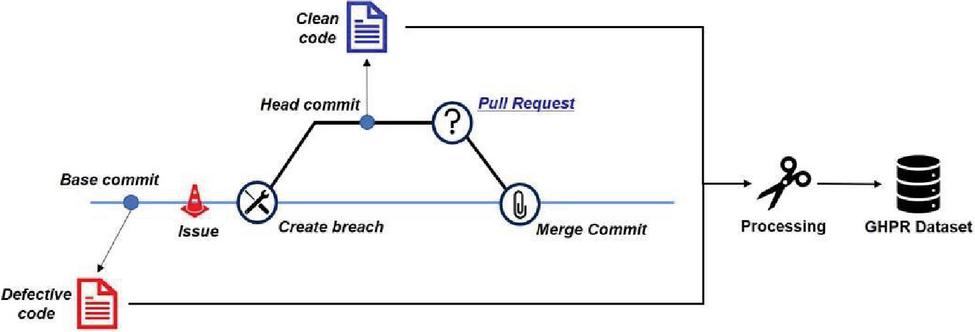
Figure 1 GHPR-based GitHub workflow.

We implement a Python script for generating a dataset using GHPR based on ghprtools.¹ The ghprtools only gather meta-information on PRs and the related issues, so we utilize RESTful GitHub API² to enhance the ghprtools to collect defective and clean source code pairs. Figure 2 shows the flowchart of the implemented script. It consists of three stages and generates a dataset of a GitHub repository as a result. The dataset comprises pairs of instances with a PR message in NL, a short description of the PR, and a defective or non-defective source code in a PL by function level. The details of each stage are as follows.

(1) Preparing stage: This requires a URL of a GitHub repository. Then, it makes a list of PRs enrolled in the repository using the RESTful GitHub API.

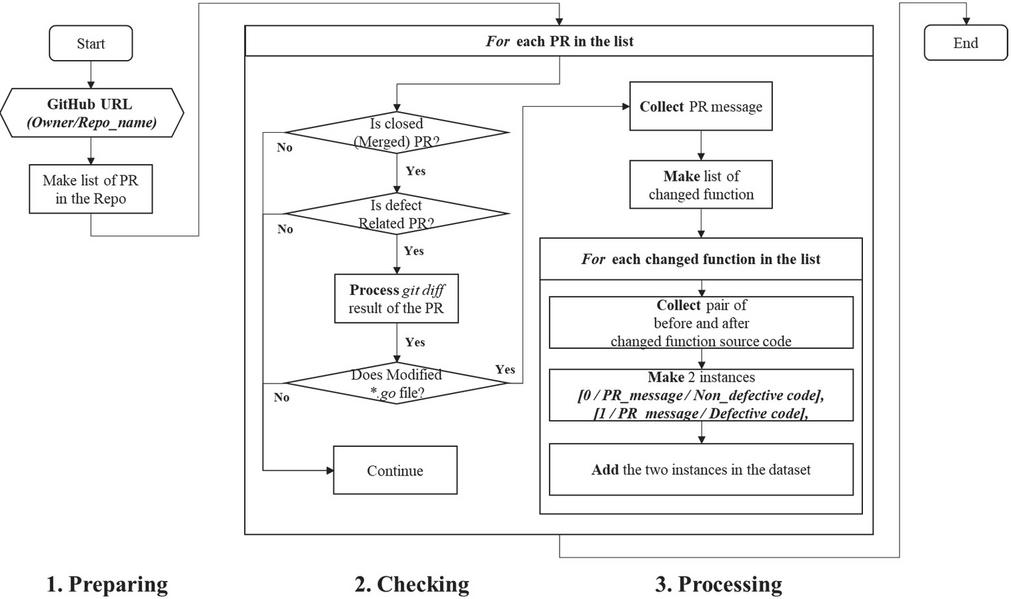
Figure 2 Flowchart of generating a defect dataset using GHPR.

(2) Checking stage: This collects defect-related PRs through three checks. First, it checks if each PR in the list is a closed state, which means the PR is merged into a main branch. Second, it checks if the closed PR is related to a defect. We check if the message of each PR includes defect-related keywords (e.g., fix, solve, resolve, and bug) and excludes non-defect-related keywords (e.g., document, typo, golint). Then, it checks if the PR modifies ‘.go’ files through git diff result of the PR because we only focus on Go.

(3) Processing stage: This collects the message of the PR and makes a list of changed functions through the git diff result of the PR. Then, it collects a pair before and after the changed function’s source code in the list. After that, it makes two instances with a class label (i.e., 0 or 1), the PR message in NL, and defective or non-defective source code written in Go. Finally, the two instances are added to a dataset.

Since the three pre-trained models applied in this study were trained on a large function-level large corpus, we generate datasets at the function level. In addition, due to the limitations on the maximum number of input tokens into the models and the capacity of the graphics card we used for deep learning, we collect only functions with changes within 400 tokens in the source code.

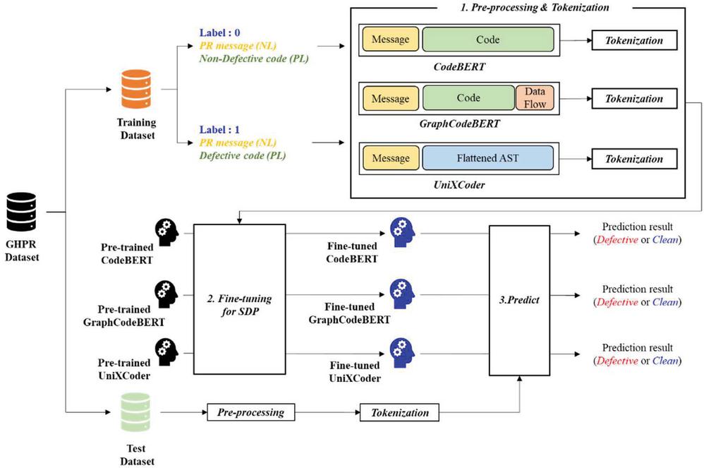
Figure 3 Workflow of generating JIT SDPs based on pre-trained models.

3.2 Function Level JIT SDP Based on a Pre-trained Model

We implement function-level JIT SDP models by fine-tuning pre-trained models (i.e., CodeBERT, GraphCodeBERT, and UniXcoder), which are available on the HuggingFace³ website. Each model has a pre-trained model for classification tasks (i.e., CodeSearch, and Clone Detection), and we fine-tune the model on the defect-related dataset using GHPR to make the JIT SDP model. The overall workflow of generating JIT SDP models based on the pre-trained models is shown in Figure 3.

(1) Pre-processing and tokenization: Each pre-trained model has a different input sequence, as shown in Section 2.3. After converting a pair of PR message and source code to each model’s suitable input type, the converted input is tokenized using each model’s tokenizer.

(2) Fine-tuning for SDP: Each pre-trained base model is fine-tuned on each converted and tokenized input.

(3) Prediction: Each function in the testing dataset follows the same pre-processing and tokenization process, depending on each model. Then, each model predicts the defect-proneness of the function.

4 Experimental Setup

4.1 Research Questions

This study establishes three research questions, and the reasons for the establishment are as follows. First, it is the first attempt to compare the performance of the SDP models based on different pre-trained models targeting edge-cloud systems. Thus, we establish RQ1 to confirm the most appropriate pre-trained model in the within-project environment (i.e., WPDP) where training and test datasets are included in a project. Second, the applicable timing of the SDP model can be judged through the model’s prediction performance according to the amount of training data. In other words, it is important to check the minimum amount of training data that shows stable prediction performance. Thus, we set RQ2 to confirm the change in the model’s prediction performance by changing the amount of training data in the WPDP environments. Third, the cross-project environment (i.e., CPDP), where training and test datasets come from different projects, can solve WPDP’s limitations from the burden of simultaneous development and data collection for generating the SDP model. Thus, we set RQ3 to confirm the applicability of SDP models based on the pre-trained models and the most appropriate pre-trained model in the CPDP environments. The three research questions are as follows.

(1) RQ1: Which pre-trained model is the most appropriate in the WPDP environment on edge-cloud systems?

(2) RQ2: How much does the performance of SDP models based on pre-trained models change depending on the amount of training data in the WPDP environment?

(3) RQ3: Which pre-trained model-based SDP model is the most appropriate in the CPDP environment on edge-cloud systems?

4.2 Subject Projects

Since our GHPR-based dataset generation method works on repositories registered on GitHub, we search projects written in Go on GitHub with edge-cloud related keywords (e.g., edge, cloud, and IoT). Among the 117 results, we remove non-serious projects (e.g., homework assignments) with less than 1K stars and 400 forks. After that, we select four projects implemented in Go over 90% with more than 1K closed PRs. The characteristics and short descriptions of the projects are described in Table 1.

Table 1 Characteristics of subject projects

Name	Starts	Forks	PRs	Short Description
EdegeX-go(EdgeX) $^{1}$	1.1K	0.4K	2.3K	Open source project building a common open framework for IoT edge computing.
Kubeedge (Kube) $^{2}$	5.5K	1.4K	2.6K	Open source system for extending native containerized application to hosts at Edge.
Openshift $^{3}$	1.3K	1.2K	5.3K	Application platform to manage hybrid cloud, multi-cloud, and edge deployments managed by Red Hat.
Traefik $^{4}$	40.5K	4.4K	4.2K	The Cloud Native Application Proxy works with Docker and Kubernetes.
$^{1}$ https://github.com/edgexfoundry/edgex-go $^{2}$ https://github.com/kubeedge/kubeedge $^{3}$ https://github.com/openshift/installer $^{4}$ https://github.com/traefik/traefik

4.3 Fine-tuning Settings for Pre-trained Models

We generate SDP models by fine-tuning the pre-trained models and utilize same fine-tuning settings as the settings of each original paper [7–9], except for the batch size and max sequence length due to the memory limitation. We set the max sequence length as 450 (i.e., 50 tokens for PR message, 400 tokens for source code), and batch size as 8. We use the Adam optimizer to update the parameters.

Table 2 Confusion matrix

	Predict as Defective	Predict as Clean
Actually defective	TP	FN
Actually clean	FP	TN

4.4 Evaluation Metrics

We adopt two types of performance metrics. First, we calculate two commonly used metrics (i.e., AUC and F-measure) in SDP studies, to confirm the conventional prediction performance of the model. Second, we adopt FIR (file inspection reduction) and CIR (cost inspection reduction) to confirm each model’s cost and effort effectiveness. All four metrics can be calculated based on Table 2. In addition, except for CIR, three other metrics need to be maximized. The definitions and equations for each metric are as follows.

(1) AUC (area under the receiver operating characteristic curve): This is an area under the curve between the true-positive and false-positive rate, and it is independent of the cut-off value. The performance of the model is categorized into five classes according to the AUC; Excellent (0.9–1.0), Good (0.8–0.9), Normal (0.7–0.8), Poor (0.6–0.7), and Fail (0.5–0.6). In addition, 0.5 AUC means that the model’s the prediction performance is the same as random selection model.

(2) F-measure: This is the harmonic mean of precision ( $p r e c = \frac{T P}{T P + F P}$ ) and recall (recall $=$ $\frac{T P}{T P + T N})$ . Precision focuses on where actual defective functions are predicted as defective functions, and recall focuses on where actual defective functions are predicted as non-defective functions. F-measure seeks a balance of them.

F-measure = \frac{2 P r e c \times R e c a l l}{P r e c + R e c a l l} .

(3) FIR (file inspection reduction): Shin et al. (2010) [21] propose this metric to calculate reduced effort according to the prediction results. It is the ratio of the reduced number of functions to inspect using a prediction model compared to a random selection to obtain the same precision. When FI (file inspection) is $F I = \frac{T P + F P}{T P + T N + F P + F N}$ , FIR is defined as follows.

F I R = \frac{P D - F I}{P D} .

(4) CIR (cost inspection reduction): Zhang and Cheung (2013) [28] proposed this metric to calculate the cost of defect prediction. CIR is the ratio of the cost to inspect using a prediction model compared to the cost to inspect all function. Assuming the average inspection cost for the defective module is C $_{i}$ , the average cost of missing a defective module $C_{f n}$ , and $C_{i} / C_{f n} = 1 / 3$ . The CIR is defined as follows.

CIR = \frac{C_{i} \times (T P + F P) + C_{f n} \times F N}{C_{i} \times (T P + F P + F N + T N)} .

5 Experimental Results

5.1 RQ1: Which Pre-trained Model is the Most Appropriate in WPDP Environment on Edge-cloud Systems?

Approach: We randomly divide each dataset into training and test data with a ratio of 7:3. Then, for making the validation dataset, we re-divide the training dataset into a training and validation dataset with a ratio of 7:3. Lastly, we fine-tuned each pre-trained model to generate an SDP model using the same training dataset. For testing, we feed all test datasets to the best-performing model on the validation dataset among eight epochs.

Table 3 Performance of three SDP models in four projects in the WPDP environment

	CodeBERT	GraphCodeBERT	UniXCoder
1. AUC
EdgeX	0.764	0.676	0.811
Kube	0.502	0.841	0.889
Openshift	0.923	0.909	0.917
Traefik	0.513	0.545	0.434
2. F-measure
EdgeX	0.669	0.688	0.702
Kube	0.667	0.790	0.782
Openshift	0.821	0.823	0.831
Traefik	0.670	0.600	0.667
3. FIR
EdgeX	0.200	0.104	0.288
Kube	0.003	0.243	0.326
Openshift	0.310	0.318	0.325
Traefik	0.008	0.002	0.003
4. CIR
EdgeX	0.995	0.957	0.952
Kube	1.002	0.768	0.818
Openshift	0.760	0.732	0.719
Traefik	1.003	1.119	1.002

Finding: Table 3 shows the performance measurement results of four metrics of each SDP model based on a pre-trained model. The bold fonts are the highest performance among the three SDP models on a project. As shown in Table 3, UniXcoder achieves the best performance in 10 cases among 16 cases (i.e., 4 metrics $\times$ 4 subject projects). It indicates that UniXcoder achieves better performance than other models. We assume that the reason for the outperformance of UniXcoder is that the converted AST information from the source code, which is the input data format of UniXcoder, is more effective in identifying defects than a sequence of source code tokens, which is the input data format of CodeBERT and GraphCodeBERT.

In the case of AUC, UniXcoder achieves good and excellent prediction performance except for Traefik. In addition, it achieves above 0.7 F-measure scores on three projects (i.e., EdgeX, Kube, and Openshift), which is a relatively acceptable performance, although F-measure does not have a performance criterion like AUC. In the case of FIR, UniXcoder achieves 28% to 32% of those of others on three projects (i.e., EdgeX, Kube, and Openshift). It indicates that UniXcoder is more effort-effective than others. Similarly, in the case of CIR, UniXcoder achieves 5% to 28% of those of others on three projects (i.e., EdgeX, Kube, and Openshift). It also indicates that UniXcoder is more cost-effective than the others.

In addition, the collected dataset through GHPR is class-balanced (i.e., clean code:defective code $=$ 1:1), and it is favourable to the random selection model. As shown in Table 3, UniXcoder shows better performed than the random selection model (i.e., AUC $>$ 0.5, FIR $>$ 0, and CIR $<$ 1). Thus, we can indirectly confirm that the UniXcoder-based model can recognize the source code’s defect pattern and effectively determine a function’s defectiveness in terms of cost and effort. In conclusion, we can confirm UniXCoder has better performance than other models, and its performance is applicable in the within-project environment.

However, in the case of the Traefik project, the three models show the performance similar to (i.e., AUC $=$ 0.5, FIR $=$ 0, and CIR $=$ 1) or worse than (i.e., AUC $<$ 0.5, FIR $<$ 0, and CIR $>$ 1) that of the random selection model. We assume the reason for the poor performance is that the Traefik dataset is not sufficiently collected, so each model cannot learn about defects in the project, and the detailed analysis is in Section 6.

5.2 RQ2: How Much Does the Performance of the SDP Models Based on Pre-trained Models Change Depending on the Amount of Training Data in WPDP Environment?

Approach: We randomly generate a training dataset by changing from 30% to 70% of a subject dataset. Then, from the remained dataset, we randomly select by the number of 30% of the subject dataset as the test dataset. Lastly, we fine-tuned each pre-trained model for generating SDP model using the same training dataset with various ratios. Finally, for testing, we feed all test datasets to the best-performing model on the validation dataset among eight epochs.

Finding: Figures 4, 5, 6 and 7 show the performance changes according to the amount of training data for AUC, F-measure, FIR, and CIR, respectively. The higher AUC, F-measure, and FIR mean better performance, and closer to the top of the graph indicates better performance. Conversely, in the case of CIR, a lower value means better performance, so the closer to the bottom of the graph, the better the performance.

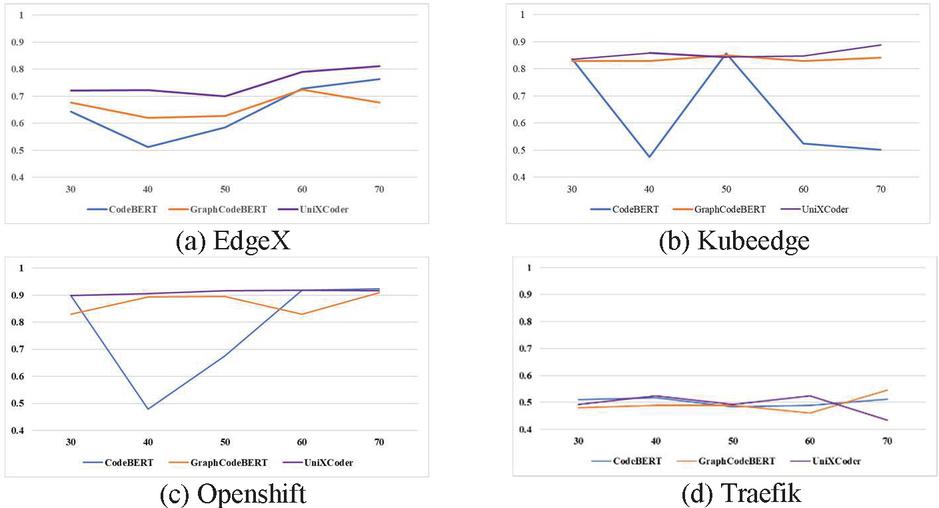
Figure 4 AUC changes according to the amount of training data.

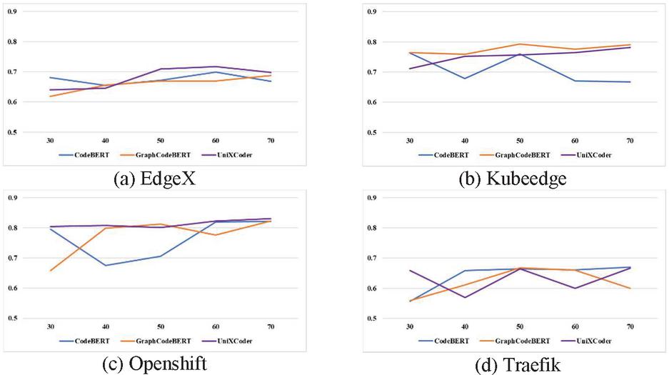
Figure 5 F-measure changes according to the amount of training data.

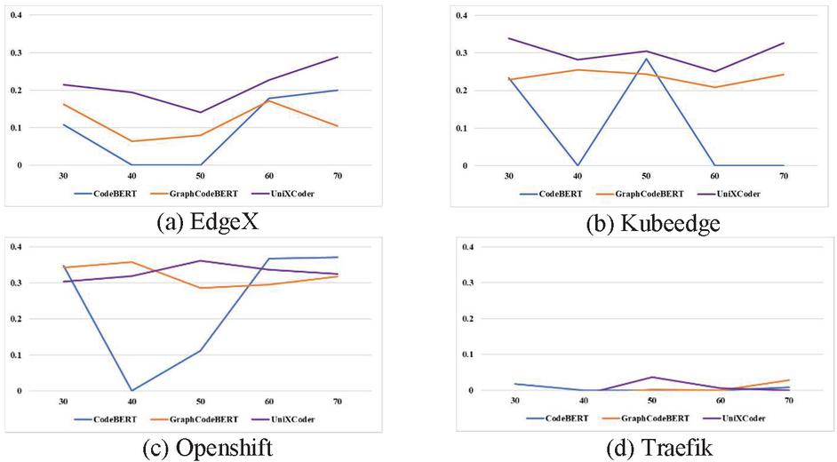
Figure 6 FIR changes according to the amount of training data.

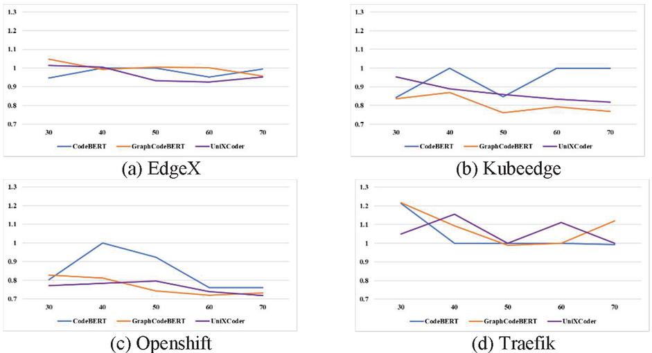
Figure 7 CIR changes according to the amount of training data.

First, as shown in Figures 4 and 6, except for Traefik, AUC and FIR of UniXcoder are closer to the top of the graph than other models. This indicates that UniXcoder has better prediction performance and is more effort-effective than other models over various numbers of training data. In addition, the performance variation over the various numbers of training data is also smaller than others. It shows that UniXcoder can learn defect-related information more efficiently using smaller training data than other models.

Second, as shown in Figures 5 and 7, the best model for CIR and F-measure differs depending on the subject project and the amount of training data. However, GraphCodeBERT and UniXcoder mainly show better prediction performance and are more cost-effective than CodeBERT, except Traefik. Similarly, in terms of performance variation over the various numbers of training data, the performance variation of GraphCodeBERT and UniXcoder is smaller than CodeBERT. It also indicates that GraphCodeBERT and UniXcoder can learn more efficiently using smaller training data than CodeBERT. In summary, UniXcoder is the most suitable pre-trained model among others in the WPDP environment because it has similar or better performance and less performance variation than other models according to the amount of training data. In conclusion, we can confirm that the UniXcoder-based SDP model can be used in the WPDP environment at early timing compared to other models.

However, the same as RQ1, the three models’ performances are similar to, or worse than, the random selection model over various numbers of training data in the case of Traefik. We re-confirm that the Traefik dataset is not sufficiently collected, so each model cannot learn about defects in the project, and the detailed analysis is in Section 6.

5.3 RQ3 Which Pre-trained Model-based SDP Model is the Most Appropriate in CPDP Environment on Edge-cloud Systems?

Approach: To implement CPDP environment, among the four subject projects, we choose a project as the source project and pick another project as the target project. Then, we choose the best performance model based on the source project in RQ1. After that, we re-evaluate the model’s performance using the test data of the target project used in RQ1. We exclude Traefik as a source project that does not show better performance than the random selection model.

Table 4 Performance of three SDP models in the CPDP environment

(Source $\to$ Target)	CodeBERT	GraphCodeBERT	UniXCoder
1. AUC
EdgeX $\to$ Kube	0.494	0.516	0.482
EdgeX $\to$ Openshift	0.507	0.488	0.502
EdgeX $\to$ Traefik	0.520	0.491	0.498
Openshift $\to$ EdgeX	0.510	0.483	0.508
Openshift $\to$ Kube	0.514	0.455	0.509
Openshift $\to$ Traefik	0.510	0.501	0.485
Kube $\to$ EdgeX	0.548	0.526	0.525
Kube $\to$ Openshift	0.537	0.494	0.507
Kube $\to$ Traefik	0.506	0.510	0.478
2. F-measure
EdgeX $\to$ Kube	0.468	0.655	0.655
EdgeX $\to$ Openshift	0.614	0.653	0.571
EdgeX $\to$ Traefik	0.616	0.637	0.529
Openshift $\to$ EdgeX	0.568	0.638	0.649
Openshift $\to$ Kube	0.613	0.657	0.668
Openshift $\to$ Traefik	0.585	0.644	0.643
Kube $\to$ EdgeX	0.667	0.662	0.599
Kube $\to$ Openshift	0.666	0.666	0.650
Kube $\to$ Traefik	0.667	0.665	0.623

Finding: Table 4 shows the performance of each model on different combinations of source and target project. As shown in Table 4, no source or target project combination performs better than the random selection model. We assume the reason for the poor performance of all CPDP models is that source and target projects differ in the styles and details of the source code between source and target projects, although the source and target projects are both related to the edge-cloud system. Thus, we confirm the necessity of pre-processing techniques that minimize the different properties of the two projects and emphasize the similar properties for CPDP. In addition, UniXcoder, which shows better performance than other models in RQ1 and RQ2, shows worse performance than others. We assume that UniXcoder is overfitted in a source project, so it is not efficient in predicting defects in other projects. Thus, we confirm the necessity of a method to prevent a model from being overfitted for a project for CPDP.

In conclusion, we can confirm that additional research is needed to apply our model in cross-project environment.

6 Discussion

The three models’ prediction performance on Traefik is significantly lower than other subject projects. We assume that the reason for the poor performance is that the collection of data was not sufficient to learn defects. Accordingly, we analyse each dataset on the number of PR, modified files, functions, and words in PR message.

Table 5 shows the result of analysing each dataset. ‘# of PRs’ indicates the total number of defect-related PRs in the dataset, ‘# of modified files’ indicates the total number of modified files to resolve defects in the dataset, ‘# of modified functions’ indicate the total number of modified functions to resolve defects, and ‘# of words in PR messages’ indicate the total number of words of PR messages, which are the short description of the PR. The last three rows indicate the number of functions and words per PR, file, and function. As shown in Table 5, in the case of the number of functions per file, Traefik has 70% of EdgeX, which have the fewest number of functions and 14% of Openshift, which has the highest number of functions. In addition, in the case of the number of functions per a file, Traefik only has 81% of EdgeX and 59% of Openshift. In summary, Traefik has a smaller number of functions per PR and file; in other words, the amount of training data for a model to learn a defect is less than others. Thus, we assume that the prediction performance is degraded because the number of functions in a PR and file is insufficient, so each model cannot learn defects in the PR. In addition, the number of words per function is also small compared to other projects. In other words, the description of a PR is less specific than others. Thus, we assume that it also affects the poor performance.

In conclusion, we confirm that the amount of collected data and its analysis are absolutely necessary when creating a WPDP defect prediction model using a pre-trained model.

Table 5 Analysing results on four datasets

	EdgeX	Kube	Openshift	Traefik
# of PRs	312	256	320	419
# of modified files	1664	1535	5804	1911
# of modified functions	3828	4640	18,476	3600
# of words in PR messages	33,408	33,448	297,734	20,902
# of functions Per PR	12.269	18.125	57.737	8.591
# of functions Per file	2.300	3.022	3.183	1.883
#of words Per function	8.727	7.208	6.114	5.806

7 Threats to Validity

7.1 Internal Validity

We utilize the same fine-tuning parameter as the original papers [7–9], and changed the maximum number of tokens to input, so the performance can be changed depending on the settings. In addition, we generate datasets through GHPR on actively under development projects, so the instances of the datasets can be changed according to the execution time of crawling.

7.2 External Validity

We study four subject projects that are publicly opened on GitHub. Generally speaking, only four projects are not enough to show the generalizability of our findings. We tried to find as many collectible projects as possible, and we will generate more datasets and apply them to our models in future work to alleviate this validity.

7.3 Construct Validity

We only evaluated our model on the dataset collected through GHPR. However, since the dataset collected through GHPR (i.e., class-balanced) is different from the data collected in the actual development environment (i.e., class-imbalanced), there may be differences from the measured performance in this study when applied to an actual ongoing project. Thus, in future work, we will check our model’s performance according to the actual development scenario.

8 Conclusion

An edge-cloud system is a framework that distributes computing power closer to clients or devices in the computing environment. However, as in traditional systems, the amount of resource for testing the system is always limited. We propose a function-level JIT SDP model based on pre-trained model for the edge-cloud systems. In this study, we compare and analyse the prediction performance of the SDP models based on the three popular pre-trained models (i.e., CodeBERT, GraphCodeBERT, and UniXCoder) on the four open source edge-cloud systems in the WPDP and CPDP environment. As a result, we can confirm UniXcoder is the most suitable pre-trained model among them in the WPDP environment. In addition, we can confirm that additional research is needed to apply the SDP models based on the pre-trained models in the CPDP environment.

In future work, we will analyse the performance change according to the quality and amount of collected data to give developers guidelines to apply our model. In order to apply our model to the CPDP environment, we will apply transfer learning and few-shot learning that alleviates differences between source and target projects.

Acknowledgements

This research was supported by the National Research Foundation of Korea (NRF-2020R1F1A1071888), the Ministry of Science and ICT (MSIT), Korea, under the Information Technology Research Center (ITRC) support program supervised by the Institute of Information & Communications Technology Planning & Evaluation (IITP-2022-2020-0-01795), and the Basic Science Research Program through the National Research Foundation of Korea (NRF) funded by the Ministry of Education (NRF- 2022R1I1A3069233).

References

[1] E. N. Akimova, et al., “PyTraceBugs: A large Python code dataset for supervised machine learning in software defect prediction,” in 2021 28th Asia-Pacific Software Engineering Conference (APSEC), 2021, pp. 141–151.

[2] M. Bakaev, et al. (eds.) “ICWE 2021 International Workshops, BECS and Invited Papers, Biarritz. France, 2021” in Revised Selected Papers. Springer Nature, 2022.

[3] M. V. R Blondet, et al., “A wearable real-time BCI system based on mobile cloud computing,” in 2013 6th International IEEE/EMBS Conference on Neural Engineering (NER), 2013, pp. 739–742.

[4] E. H. Butterfield, “Fog computing with Go: A comparative study,” CMC Senior Thesis, Claremont College, 2016.

[5] R. Buyya and N. S. Satish (eds.) Fog and Edge Computing: Principles And Paradigms, John Wiley & Sons, 2019.

[6] J. Deng, L. Lu, Q. Shaojian, “Software defect prediction via LSTM,” IET Software, vol. 14, no. 4, pp. 443–450, 2020.

[7] Z. Feng, et al., “Codebert: A pre-trained model for programming and natural languages,” arXiv preprint arXiv:2002.08155, 2020.

[8] D. Guo, et al., “UniXcoder: Unified cross-modal pre-training for code representation,” arXiv preprint arXiv:2203.03850, 2022.

[9] D. Guo, et al., “Graphcodebert: Pre-training code representations with data flow,” arXiv preprint arXiv:2009.08366, 2020.

[10] S. Herbold, A. Trautsch, J. Grabowski, “A comparative study to benchmark cross-project defect prediction approaches,” in Proceedings of the 40th International Conference on Software Engineering, 2018, pp. 1063–1063.

[11] H. Husain, et al., “Codesearchnet challenge: Evaluating the state of semantic code search,” arXiv preprint arXiv:1909.09436, 2019.

[12] C. Khanan, et al., “JITBot: an explainable just-in-time defect prediction bot,” in Proceedings of the 35th IEEE/ACM International Conference on Automated Software Engineering, 2020, pp. 1336–1339.

[13] S. Kwon, et al., “CodeBERT based software defect prediction for edge-cloud systems,” in 2nd International Workshop on Big Data Driven Edge Cloud Services (BECS 2022), International Society for Web Engineering, 2022.

[14] J. Li, et al., “Software defect prediction via convolutional neural network,” in 2017 IEEE International Conference on Software Quality, Reliability and Security (QRS), IEEE, 2017, pp. 318–328.

[15] Z. Li, et al., “CodeReviewer: Pre-training for automating code review activities,” arXiv preprint arXiv:2203.09095, 2022.

[16] E. Mashhadi and H. Hemmati, “Applying codebert for automated program repair of java simple bugs,” in 2021 IEEE/ACM 18th International Conference on Mining Software Repositories (MSR), IEEE, 2021, pp. 505–509.

[17] F. F. S. B. De Matos, P. A. L. Rego, F. A. M. Trinta, “An empirical study about the adoption of multi-language technique in computation offloading in a mobile cloud computing scenario,” in 11th International Conference on Cloud Computing and Services Science, 2021, pp. 207–214.

[18] C. Pan, M. Lu, B. Xu, “An empirical study on software defect prediction using codebert model,” Applied Sciences, vol. 11, no. 11, p. 4793, 2021.

[19] S. K Pandey, R. B. Mishra, A. K. Tripathi, “Machine learning based methods for software fault prediction: A survey,” Expert Systems with Applications, vol. 172, p. 114595, 2021.

[20] K. Shi, et al., “PathPair2Vec: An AST path pair-based code representation method for defect prediction,” Journal of Computer Languages, vol. 59, p. 100979, 2020.

[21] Y. Shin, et al., “Evaluating complexity, code churn, and developer activity metrics as indicators of software vulnerabilities,” IEEE Transactions on Software Engineering, vol. 37, no. 6, pp. 772–787, 2010.

[22] R. S. Wahono, “A systematic literature review of software defect prediction,” Journal of Software Engineering, vol. 1.1, pp. 1–16, 2015.

[23] J. Xu, et al., “ACGDP: An augmented code graph-based system for software defect prediction,” IEEE Transactions on Reliability, vol. 71, no. 2, 2022.

[24] J. Xu, F. Wang, J. Ai, “Defect prediction with semantics and context features of codes based on graph representation learning,” IEEE Transactions on Reliability, vol. 70, no. 2, pp. 613–625, 2020.

[25] J. Xu, et al., !A GitHub-based data collection method for software defect prediction,” in 2019 6th International Conference on Dependable Systems and Their Applications (DSA), IEEE, 2020, pp. 100–108.

[26] X. Yang, et al., “Deep learning for just-in-time defect prediction,” in 2015 IEEE International Conference on Software Quality, Reliability and Security, IEEE, 2015, pp. 17–26.

[27] F. Zhang, et al., “Improving stack overflow question title generation with copying enhanced CodeBERT model and bi-modal information,” Information and Software Technology, vol. 148, pp. 106922, 2022.

[28] H. Zhang and S. C. Cheung, “A cost-effectiveness criterion for applying software defect prediction models,” in Proceedings of the 2013 9th Joint Meeting on Foundations of Software Engineering, 2013, pp. 643–646.

[29] X. Zhou, D. Han, D. Lo, “Assessing generalizability of CodeBERT,” in 2021 IEEE International Conference on Software Maintenance and Evolution (ICSME), IEEE, 2021, pp. 425–436.

[30] Y. Zhou, et al., “How far we have progressed in the journey? An examination of cross-project defect prediction,” ACM Transactions on Software Engineering and Methodology (TOSEM), vol. 27, no. 1, pp. 1–51, 2018.

Footnotes

¹https://github.com/soroushj/ghpr-tools

²https://docs.github.com/en/rest

³https://huggingface.co/

Biographies

Sunjae Kwon received the bachelor’s degree in electric engineering from Korea Military Academy in 2009, the master’s degree in computer engineering from Maharishi Markandeshwar University in 2015. He is a doctoral student in software engineering from KAIST. His research areas include software analytics based on AI, software defect prediction, mining software repositories, and software reliability engineering.

Sungu Lee received the bachelor’s degree in mathematics from KAIST in 2021, the master’s degree in software engineering from KAIST in 2022. He is a doctoral student in software engineering from KAIST. His research areas include software analytics based on AI, software defect prediction, mining software repositories, and software reliability engineering.

Duksan Ryu earned a bachelor’s degree in computer science from Hanyang University in 1999 and a Master’s dual degree in software engineering from KAIST and Carnegie Mellon University in 2012. He received his Ph.D. degree in school of computing from KAIST in 2016. His research areas include software analytics based on AI, software defect prediction, mining software repositories, and software reliability engineering. He is currently an associate professor in software engineering department at Jeonbuk National University.

Jongmoon Baik received his B.S. degree in computer science and statistics from Chosun University in 1993. He received his M.S. degree and Ph.D. degree in computer science from University of Southern California in 1996 and 2000 respectively. He worked as a principal research scientist at Software and Systems Engineering Research Laboratory, Motorola Labs, where he was responsible for leading many software quality improvement initiatives. His research activity and interest are focused on software six sigma, software reliability & safety, and software process improvement. Currently, he is an associate professor in school of computing at Korea Advanced Institute of Science and Technology (KAIST). He is a member of the IEEE.