A Study and Analysis of a New Hybrid Approach for Localization in Wireless Sensor Networks
Rupendra Pratap Singh Hada, Uttkarsh Aggarwal and Abhishek Srivastava*
Department of Computer Science and Engineering, Indian Institute of Technology Indore, India
E-mail: phd2101101004@iiti.ac.in; uttkarsh.agg2409@gmail.com; asrivastava@iiti.ac.in
*Corresponding Author
Received 30 December 2022; Accepted 04 February 2023; Publication 16 June 2023
Abstract
Accurate localization of nodes in a wireless sensor network (WSN) is imperative for several important applications. The use of global positioning systems (GPS) for localization is the natural approach in most domains. In WSNs, however, the use of GPS is challenging because of the constrained nature of deployed nodes as well as the often inaccessible sites of WSN nodes deployment. Several approaches for localization without the use of GPS and harnessing the capabilities of the received signal strength indicator (RSSI) exist in literature, but each of these makes the simplifying assumption that all the WSN nodes are within the communication range of every other node. In this paper, we go beyond this assumption and propose a hybrid technique for node localization in large WSN deployments. The hybrid technique comprises a loose combination of a machine learning (ML) based approach for localization involving random forest and a multilateration approach. This hybrid approach takes advantage of the accuracy of ML localization and the iterative capabilities of multilateration. We demonstrate the efficacy of the proposed approach through experiments on a simulated set-up and follow it up with a feasibility demonstration through a prototypical implementation in the real world.
Keywords: Localization, random forest, multilateration.
1 Introduction
A wireless sensor network (WSN) is an infrastructure-less, self-configured network of sensor nodes that communicate with each other via radio signals. Each node in a WSN is laden with sensors of various kinds and these are often deployed in terrains that are dangerous and inaccessible for humans. A sensor node once deployed in such terrains is on its own with limited energy and computational resources with no means of replenishing these. The aim, therefore, is to minimize energy expenditure and prolong the useful life of nodes. In such circumstances, localization of sensor nodes in WSN is an important issue. This is because the usual localization approach in outdoor locations using global positioning systems (GPS) is unfeasible. GPS comprises modules that are resource intensive and deploying these over WSN nodes shortens the latter’s life significantly. In addition to this, the geographical locations in which such nodes are deployed often do not facilitate the proper functioning of GPS modules. This is exemplified in a project of ours wherein we are deploying a WSN in the Melghat Tiger Reserve, a thickly forested area in Central India, to detect forest fires. Although the WSNs work well and warn of a fire effectively, determining the location of the fire is non-trivial. GPS modules do not work here, not just owing to their heavy nature, but also because of the thickly wooded environment that disrupts GPS signals and makes them ineffective.
Outdoor localization without the use of GPS is broadly classified into range-free [1], and range-based [2] localization. Both these localization schemes work on the premise that there are certain nodes in the network whose correct locations are known. Such nodes are called anchor nodes and based on these the locations of the other nodes are computed. In realistic scenarios, like our project on forest fires, anchor nodes are usually the ones deployed in parts of the terrain that are more accessible (for example the periphery of the forested area in our project) where a GPS device can be used to determine the correct location. Such anchor nodes in most cases are few and far between and need to be utilized effectively to localize the majority of the remaining nodes. In range-free localization, the approach is to utilize simple data like the ‘number of hops’ between the anchor nodes and the node being localized, to get a rough idea on the location of the node. The important point is that no additional hardware is utilized at any of the nodes to facilitate range-free localization. The advantage of this approach is its simplicity and cost-effectiveness. The downside, however, is the low accuracy of localization. Two examples of approaches employing range-free localization are Centroid [3] and DV-hop [4].
Range-based localization on the other hand requires additional hardware for transmission and reception of signals at each node. In a WSN network this hardware is already available at each node and hence range-based localization becomes convenient. Range-based localization involves an assessment of the signals received at unknown nodes from anchor nodes and the strength, angle, arrival-time of such signals is utilized to assess the position of the node. The angle of arrival [5], time of arrival [6], and received signal strength indicator (RSSI) [7] are popular approaches that utilize range-based localization techniques.
In this paper, we utilize a range-based technique, more specifically the received signal strength indicator (RSSI) technique for localization. A high-level depiction of the use of RSSI for localization is shown in Figure 1(a). Anchor nodes whose locations are known in advance transmit signals that are received by the node to be localized. The strength of the received signals from different anchor nodes are analysed using various algorithms. Based on this, the position of the node is determined.

Figure 1 (a) Demonstrates the working of RSSI localization method. (b) Demonstrates the deployment in the proposed method.
The algorithms used to analyse RSSI values and localize nodes are broadly classified into those employing machine learning (ML) techniques and those based on more conventional techniques like multilateration [8]. ML approaches for localization using RSSI are effective but have an important limitation: they only work well as long as all the unknown nodes are within the communication range of the anchor nodes.
This means that a realistic scenario, where anchor nodes are few and there are a large number of unknown nodes far away (not within communication range) from the anchor nodes, is not catered to well. Figure 1(b) pictorially depicts this scenario. The reason ML approaches do not work well in situations where unknown nodes are far away is that this requires multiple iterations of localization. Multiple iterations of localization imply a scenario wherein the anchor nodes first localize a few unknown nodes and the newly localized unknown nodes become the new anchor nodes which are used for further localization. ML techniques need to be extensively trained to perform localization. This training works well for the first iteration of localization when training is done in advance and in an ‘off-line’ manner. Subsequent rounds of localization require ‘on-line’ training and within the resource constrained environments of the WSN nodes. Given the space and computational requirements of such training, these are not possible within WSN nodes. Hence ML algorithms cannot be used for localization in WSN with nodes spread over large areas and far away from anchor nodes.
Algorithms based on multilateration techniques are more useful in this regard and can be used for localizations that require multiple iterations. Multilateration involves assessing the RSSI values of signals from multiple anchor nodes at the unknown node. Based on these analyses, an estimation of the location of the unknown nodes is made. Several endeavours utilize multilateration for localization; these include [9, 10]. While multilateration enables localization of nodes far away from anchor nodes through multiple iterations, its major drawback is lack of accuracy.
In this paper, we overcome the issues of both ML based localization techniques and multilateration based techniques by adopting a ‘hybrid’ approach wherein the ML and multilateration techniques are combined. The idea is to first employ a pre-trained ML algorithm to localize a large number of unknown nodes that are within the communication range of anchor nodes. Subsequently, these newly localized nodes, which are large in number and precisely localized, are used to localize subsequent unknown nodes using multilateration. The number of iterations of multilateration is reduced significantly because of the initial localization by the ML based approach. We try several ML approaches for the initial localization and ultimately choose random forest [11] as this gives the best results.
The remainder of this paper is organized as follows: Section 2 includes a comprehensive discussion on existing work related to localization in such environments; Section 3 is a detailed discussion of the method proposed in this paper; the proposed method is validated through experiments in Section 4; and finally Section 5 concludes the paper with pointers to future work.
2 Related Work
There is extensive literature on localization techniques in WSNs and in other domains that utilize RSSI as the basis for their endeavours. Several proposed techniques directly harness RSSI for localization and appropriately optimize and refine the results. Others employ ML techniques for more accurate results. We discuss a few endeavours in this section.
[12] proposed a support vector machine (SVM) algorithm which regards the localization of nodes in a WSN as a regression problem. RSS values are used as inputs to train the model. The position prediction model is developed in an offline manner using support vector regression (SVR).
An artificial neural network (ANN) based localization algorithm is proposed in [13]. Here RSSI values between the grid sensors and anchor nodes are used as inputs to train the neural network. The ANN develops a mapping between the RSSI values and the locations of the node. This approach is based on the assumption that all sensor nodes can directly communicate with all anchor nodes.
Similarly, two groups of algorithms for localizing sensor nodes using RSSI values of signals from anchor nodes are proposed in [14]. The first class of algorithms uses fuzzy logic and genetic algorithms, while the second class uses neural networks with the RSSI values.
The idea of using a lightweight SVR implementation is proposed in [15] wherein the original problem of regression is split into sub-problems. The algorithm progresses by splitting the entire network into a series of sub-networks, such that each regression algorithm (i.e. the sub-predictors of SVR) needs to process a small amount of data.
Low-power wide-area network (LPWAN) technologies have lately emerged as a viable alternative to scalable wireless connections in smart city applications. On a training dataset collected in two different environments, indoors and outdoors, [16] investigate the use of intelligent machine learning techniques such as support vector machines, spline models, decision trees, and ensemble learning for RSSI-based ‘ranging’ in LoRa networks. An appropriate ranging model is subsequently utilized to test the accuracy of the trilateration-based localization and tracking endeavours.
[17] use finger-printing to train a neural network to develop a median accuracy (of about 16 m to 100 m) model for outdoor localization using the very little information available over pre-5G base stations with active multi-beam antenna systems.
The localization techniques proposed in literature and briefly described here are useful and significant contributions. The main limitation of these techniques is that they mostly assume that all nodes are within the range of communication of every other node. This is a rather strong assumption and often does not hold in the real world. In this paper, we attempt to overcome this assumption and propose a hybrid technique that utilizes the accuracy of ML based localization and scalability of multilateration based localization to localize nodes much beyond the communication range of known anchor nodes.
3 Proposed Method
The method proposed in this paper is meant for localization of unknown nodes, without the use of a GPS device, in a WSN that is spread over a large area. ‘Large area’ here implies that most nodes in the WSN are not within the communication range of most other nodes owing to the large size of the area of interest. It is important to specify this as most existing localization techniques work on the assumption that each node in the WSN is within the communication range of every other node.
In this large area, we start with the assumption that the locations of a few sensor nodes, called anchor nodes, are known in advance. These anchor nodes are located at the periphery of the area of interest. This is a realistic assumption as the sensor nodes at the periphery of the WSN are usually accessible and within the reach and range of a GPS device. The sensor nodes located deep within the area of interest are usually not accessible by a GPS device because of a hostile geographical terrain and/or the presence of disrupting structures like trees, and tall buildings. It is these nodes that need to be localized.
This paper proposes a hybrid approach to localize such sensor nodes that comprises a machine learning (ML) approach combined with a more conventional multilateration approach. The ML algorithm harnessed here is random forest and it localizes a large number of unknown nodes by analysing the RSSI values of communication signals received at the unknown nodes from one or more anchor nodes. Subsequently, these newly localized unknown nodes now serve as the ‘new’ anchor nodes and are used to localize nodes deeper inside the area using multilateration. The multilateration approach is usually harnessed for more than one iteration until all unknown nodes are localized. Figure 2 is a high-level depiction of the steps followed for localization.

Figure 2 Proposed hybrid localization approach.
We now discuss the proposed approach, comprising localization using RSSI in general, analysis of RSSI using an ML algorithm (random forest), and the use of multilateration with RSSI for localization, in more detail.
3.1 Localization Using RSSI
Localization through RSSI values comprises sending low power signals from the transmitter at an anchor node (a node whose location is known) and receiving the signal using a receiver at an unknown node. The strength of the signal as received at the unknown node is assessed and analysed and conclusions are drawn on the position of the unknown node relative to the anchor node that sends the signal. The intensity of signals received at the unknown node decreases with increasing distance from the transmitting anchor node.
Equation (1) is Frii’s free space transmission equation [18] and shows that the received signal strength decreases quadratically with distance from the transmitter.
| (1) |
where is the power of the signal as received at an unknown node, is the power of the signal as transmitted at the anchor node, is the gain of the transmitter at the anchor node, is the gain of the receiver at the unknown node, is the distance between the anchor and the unknown node, and is the wavelength of the signal.
The power of the signal received at the unknown node is roughly interpreted as the received signal strength indicator (RSSI) value after incorporating factors specific to the communication technology in use. The RSSI values for signals received at unknown nodes from the various anchor nodes are collected and stored in a database. A matrix for RSSI values obtained at each node from every other node in the region of interest is constructed and a db value assigned where the receiving node is beyond the communication range of the sending node.
The RSSI values so collected are subsequently analysed by an ML algorithm (random forest in this case) and a multilateration technique for localization.
3.2 Localization Using Machine Learning
The machine learning (ML) approach to localization involves training an algorithm with data on a large number of sensor nodes. The data comprises the RSSI values of signals received at each node and the relative location of the node. The algorithm is trained in such a manner that it is able to accurately localize a node that receives relevant signals from at least three anchor nodes (anchor nodes, as mentioned earlier, are nodes whose locations are known). The larger the number of anchor nodes, better the accuracy of localization. The algorithm is trained in an ‘off-line’ manner such that it is trained before it is put to use for localizing sensor nodes.
There are a large number of ML algorithms that can be employed for the task of localization. We assessed several algorithms and, based on experiments, chose to use random forest in our work as it gave the best localization accuracy. A comparison of the localization accuracies of the ML algorithms that we experimented with is shown in Section 4 which discusses the experiments conducted.
Random forest [19] is an ensemble technique that can perform both regression and classification tasks [20]. A random forest comprises several decision trees which are tree-like structures that divide a dataset on the basis of decisions taken at each node. The decision point or split value at a node is determined as one that provides the maximum information gain. A detailed discussion on forming a decision tree is beyond the scope of this paper. The interested reader is pointed to [21]. Once trained, a decision tree is able to provide an appropriate value to a new datapoint. The random forest comprises several such decision trees and an average of the value assigned by each decision tree is assigned to the new point.
3.2.1 Data for the random forest
The first step in localization using the random forest algorithm is collection of data for training the model. The training entails teaching the model to correctly map RSSI values of signals received at a node with the 2D coordinates expressing the location of the node. The 2D coordinates of the nodes constitute the output of the random forest model. The input data consists of the RSSI values at the unknown nodes from various anchor nodes. At each unknown node , we represent the RSSI value of the signal received from anchor node as .
In the RSSI matrix, the input data corresponds to the RSSI value of the signal received at the sensor node from the anchor node; whereas an output matrix of represents the coordinates of the th sensor node. The output data comprises the coordinates of each of the unknown nodes. The training part involves the creation of a random forest and this requires labelled data for a large number of unknown nodes and corresponding anchor nodes. Depending on availability, this training data is procured from: actual deployments; from standard datasets comprising mapped RSSI values and 2D coordinates; or the data is artificially generated using Frii’s free space transmission equation [18] shown in Equation (1). In our experiments, we use artificially generated data for lack of access to an extensive deployment and the unavailability of standard datasets.
3.2.2 Data preprocessing
Prior to creation of the random forest, the data collected goes through a quick step of preprocessing. Here a new parameter called is considered for each unknown node. The parameter indicates the number of anchor nodes for which the RSSI value at the node is not db. For the creation of the random forest Only datapoints whose are considered. This is because, at least three legitimate RSSI values are required for accurate localization with random forest.
3.2.3 Creation of the random forest
To create a random forest, small bootstrap samples from the input data with are taken and a decision tree is developed with each sample. A small subset of the RSSI values at a node is considered for each tree. From this small subset of RSSI values, one RSSI value is randomly selected for the root node of the decision tree. A split point of this RSSI value is so selected that it gives the best improvement in terms of variance. For brevity, we do not dwell into the procedure for variance calculation and the interested reader is pointed to the following resource [21].
Based on the ‘best’ split point of the feature, the data is divided into two or more parts and these form the child nodes of the root. At each child node again a feature value (in this case RSSI value) is randomly chosen from the small sample and the best split point for this feature value further divides the data. This is continued until a certain number of iterations or until the data is exhausted, whichever comes first. The decision tree so created is combined with a larger random forest that comprises all such decision trees created.
The number of decision trees created in the random forest, called an -estimator is an important parameter and impacts the performance of the model. We experimented with using -estimator values of , , and . We got the best results with decision trees and used this value for further computations.
3.2.4 Testing phase
Of the legitimate RSSI data with values of , was allocated for training the model whereas was kept aside for testing the efficacy.
To test the model as well as use it with our real world implementation, the test point is made to go through each of the decision trees in the random forest. As the test data point moves through each tree and converges at a node in the tree, the – coordinates of the datapoint at the node are allocated as the coordinates of the test point.
This is repeated for all decision trees and finally an average of all the and coordinates is computed and is allocated to the test point.
3.3 Localization Through Multilateration
Multilateration [22] is a localization technique popularly used to localize vehicles in a GPS system. Multilateration depends on the relation between the distance of nodes and their relative location coordinates. To localize one node using multilateration, at least three nodes with known locations (anchor nodes in our case) within the communication range of the unknown node are required. The distance between an anchor node and the unknown is calculated using Frii’s free space transmission equation [18] shown in Equation (1) that relates the received signal strength value at the unknown node with the distance from the anchor node from which the signal was sent. This distance (which is not the exact distance but a computed approximate distance) is calculated between all the anchor nodes within the communication range of the unknown node and the unknown node. The calculated distance along with the 2D coordinates of the anchor nodes are together employed in the least squares method [23]. Figure 3(a) is a high level depiction of the localization process in multilateration.
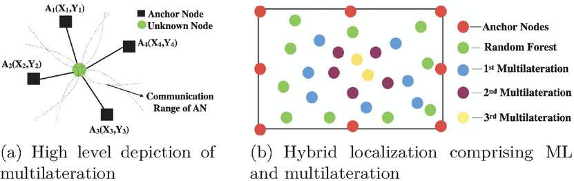
Figure 3 (a) Demonstrates the working of multilateration method. (b) Demonstrates the localization using proposed hybrid method, different colours shows the node localizations in different rounds using machine learning based localization (random forest in our case) and in multilateration approach.
Equation (2) shows the expression that needs to be minimized to compute the location of the unknown node. is the distance between the unknown node and the th anchor node as computed. The bar above indicates that the value of the distance is not necessarily exact and is diluted by channel noise, obstacles, and other shadowing effects.
| (2) |
denotes the number of anchor nodes within the communication range of the unknown node. needs to be at least for proper localization.
3.4 The Hybrid Approach to Localization
We take a hybrid approach to localization owing to limitations in the ML approach as well as the multilateration approach. The ML approach is effective in accurately localizing a large number of sensor nodes harnessing the locations of just a few anchor nodes. The limitation of the ML approach, however, is that it needs to be trained in advance and can only be employed for one iteration. It cannot be easily trained with the locations of the newly localized nodes and thus cannot be used for further iterations. The ML approach, therefore, is useful when all the unknown nodes are within the communication range of at least anchor nodes. This is usually possible in an indoor setting and is seldom the case with large outdoor locations.
The multilateration approach to localization on the other hand can be readily employed for multiple iterations. Multiple iterations imply that the unknown nodes localized in an iteration become the new anchor nodes for subsequent iterations. The iterations continue until the entire area is covered. This is useful but has the drawback that localizations through multilateration are not very precise and this imprecision increases at every iteration. A very large number of iterations of multilateration localization is therefore not advised.
The hybrid approach proposed in this paper takes the best of both approaches. One iteration of ML localization is first conducted. This results in significant number of unknown nodes getting accurately localized. These newly localized nodes become the new anchor nodes for subsequent localizations using multilateration. A combination of the two approaches enables the coverage of most of the outdoor region of interest. Figure 3(b) pictorially depicts the hybrid approach proposed in this paper. Algorithm 1 is a systematic description of the approach.
Algorithm 1 Hybrid localization
1:
2: Anchor nodes:
3: Unlocalized Sensor nodes:
4: function LOCALIZATION(, )
5: RANDOM FOREST Localization
6: nodes localized by random forest
7:
8:
9: while do
10: MULTILATERATION Localization
11: nodes localized by Multilateration
12:
13:
14: end while
15: end function
4 Evaluation
In this section we experimentally assess the working of the random forest algorithm, the multilateration approach to localization separately first, and subsequently as a hybrid combination. We first create a simulated environment to comprehensively validate the approach; and subsequently demonstrate its efficacy on a real-world set-up.
4.1 Dataset and Simulated Environment
To demonstrate the effectiveness of the proposed localization approach, we create a simulated environment and a synthetic dataset. We need to synthesize the data as standard datasets for localization over large areas do not exist. Also, we do not have access to real world deployments of this scale.
We consider a m region. A dataset comprising anchor nodes (nodes whose locations are known in advance) and sensor nodes (unknown nodes that need to be localized) deployed within this region was synthesized. A total of sensor nodes were created whose positions are along a m grid starting from a position of m from the periphery of the region of interest and extending to a distance of m. This is done along both the horizontal and vertical axes. Eight anchor nodes, whose locations are known, are placed at the periphery of the region of interest. This is a realistic scenario as nodes along the peripheries of real world regions of interest are accessible and their locations can be determined. The locations of the anchor nodes are as follows: (0,0), (60,0), (130,0), (0,60), (0,130), (60,130), (130,60), and (130,130). Each anchor node has a defined range over which it can communicate with other sensor nodes.
Out of a total of 12,321 randomly deployed sensor nodes, 3914, 4666, 3622, and 199 sensor nodes are in the communication range of precisely 3, 2, 1 and 0 anchor nodes, respectively. Based on their respective locations and distance from the anchor nodes, each sensor node has an RSSI value associated with it.
4.2 Machine Learning (Random Forest) Localization
We choose random forest as the ML algorithm for the first iteration of localization. Of the total of sensor nodes that are within the communication range of three anchor nodes (you may recall that for localization, a node needs to be receiving signals from at least three anchor nodes), of the nodes or nodes are set aside for training of the random forest and or is used for testing.
4.2.1 Localization accuracy
Figure 4 shows an overlap between the actual locations of the test sensor nodes that are localized, where red triangles denote the actual location of the nodes, and the blue squares denote the predicted location. The figure is an indication of the precision of the random forest localization as almost all the blue squares are hidden behind red triangles implying almost perfect localization.
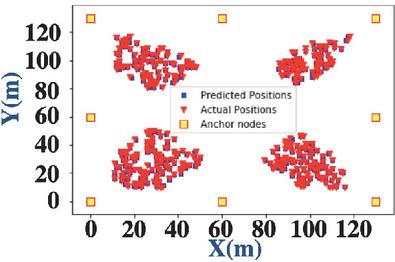
Figure 4 Overlap of predicted and actual locations of sensor nodes.
The random forest algorithm localizes 10 of the 390 sensor nodes with an average localization error of 0.20 m. Table 1 shows the localization results of the random forest algorithm for randomly selected datapoints. In this table (Xactual, Yactual) are the actual coordinates of the datapoints; (Xpred, Ypred) are the predicted coordinates using random forest localization; and Deviation indicates the distance between the actual and predicted locations. The random forest algorithm localizes sensor nodes (in Table 1) with an average, minimum and maximum localization error of 0.20 m, 0.07 m and 0.42 m, respectively.
Table 1 – coordinates, actual vs. predicted by random forest
| Xpred | Ypred | Xactual | Yactual | Deviation (m) |
| 22.97 | 16.13 | 23.0 | 16.0 | 0.13 |
| 108.99 | 19.93 | 109.0 | 20.0 | 0.07 |
| 13.85 | 34.11 | 14.0 | 34.0 | 0.18 |
| 86.88 | 23.99 | 87.0 | 24.0 | 0.17 |
| 34.15 | 93.00 | 34.0 | 93.0 | 0.15 |
| 102.75 | 97.84 | 103.0 | 98.0 | 0.29 |
| 109.76 | 98.82 | 110.0 | 99.0 | 0.30 |
| 15.79 | 35.01 | 16.0 | 35.0 | 0.21 |
| 16.02 | 31.90 | 16.0 | 32.0 | 0.10 |
| 28.73 | 85.33 | 29.0 | 85.0 | 0.42 |
4.2.2 Varying size of ‘region of interest’
We study the variation of the localization accuracy of the random forest model by changing the size of the simulated area in Figure 5(a). It is seen that as the size of the simulated area increases, keeping the number of anchor nodes and the range of communication between the anchor nodes and the sensor nodes is fixed, the localization accuracy declines sharply. This is along expected lines and shows the impact that the size of the region, within which localization is done, has on localization accuracy. As the size of the region increases, it is imperative to increase the number of anchor nodes to maintain an acceptable level of localization accuracy. This is vindicated in the following subsection where we experiment with increasing the number of anchor nodes.

Figure 5 (a) Accuracy while varying the size of field. (b) Accuracy while varying the number of anchor nodes.
4.2.3 Varying number of anchor nodes
In Figure 5(b) we study the result of changing the number of anchor nodes in a fixed size simulated area. An increase in the number of anchor nodes, with the range of communication between the anchor and the sensor nodes and the size of the simulated area (region of interest) fixed, results in a steady improvement in localization accuracy. The number of anchor nodes becomes especially important for good localization accuracy as we deal with larger regions of interest.
4.2.4 Comparison with other ML algorithms
We compare the localization performance of random forest with other known machine learning algorithms on our simulated dataset.
Table 2 Localization accuracies of various ML algorithms
| Algorithms | Error Margin () | ||
| Neural network | |||
| SVR | |||
| Decision tree | |||
| Random forest | |||
| XGBoost |
Table 2 shows the localization accuracy of the algorithm. The error margin, , in the table provides an indication of the margin of error in localization in the following manner: a datapoint (Xactual, Xactual) is considered to be correctly predicted with an error margin if for the point both the following are true:
| (3) | |
| (4) |
If both Equations (3) and (4) are true, then we consider that point to be a close point. For example 391 data points were considered as test points out of 3914 and is set to be 0.05 for which we got 379 close points out of 391 data points. The results clearly indicate the superiority of random forest in accurate localization and vindicates our choice. XGBoost [24] does perform a little better when the margin of error permitted is large. However, the performance of XGBoost rapidly deteriorates with smaller permitted margins of error.
4.3 Multilateration Localization
The other major localization approach employed in this paper is multilateration, as discussed earlier. Multilateration utilizes the least squares error technique to accurately localize nodes with distances computed from RSSI values. The advantage of the multilateration approach, in contrast to the ML localization, is that it can be used for multiple iterations. This entails starting with a set of initial anchor nodes; using these to localize unknown sensor nodes in the first iteration; the newly localized sensor nodes now become the new anchor nodes for the next iteration; localizing further unknown nodes with this new set of anchor nodes; continuing this for multiple iterations. In this way, localization is done over large ‘regions of interest’.
The downside of localization with multilateration, however, is the inferior localization accuracy as the iterations progress. The first iteration usually returns acceptable accuracy results. This deteriorates because the error in localization at earlier iteration propagates through subsequent iterations.
4.3.1 Localization over iterations
We conducted experiments to understand the extent of deterioration in localization accuracy as the iterations of localization with multilateration progress. To conduct this experiment, we use a m sized simulation environment with eight anchor nodes positioned respectively at (0,0), (25,0), (50,0), (25,50), (50,50), (0,25), (0,50), and (50,25). The sensor nodes localized in the first iteration become the new anchor nodes for the next iteration and localize more sensor nodes. In this way, the nodes over the entire region of interest are localized in three iterations. Table 3 shows the minimum, average, and maximum deviation for different iterations. The deviation values in the three tables indicate a trend towards deteriorating localization accuracy as the iterations progress.
Table 3 Deviation while localization in different iterations
| Deviation (m) | |||
| Iteration | Minimum | Average | Maximum |
| Iteration 1 | 0.08 | 0.85 | 1.10 |
| Iteration 2 | 0.82 | 1.424 | 2.57 |
| Iteration 3 | 0.62 | 1.478 | 3.00 |
4.3.2 Comparison of multilateration and random forest
As stated earlier, localization with multilateration has an advantage over random forest and other ML algorithms in terms of ease for conducting multiple iterations. The accuracy of localization with multilateration, however, is inferior to that of random forest. We compare the localization accuracy of multilateration and random forest in Table 4. The results are computed on 100 sensor nodes within an area of m, with eight anchor nodes. The superiority of random forest in terms of localization is clear from these results.
Table 4 Comparison of localization by random forest and multilateration
| Deviation (m) | |||
| Algorithm | Minimum | Average | Maximum |
| Random forest | 0.02 | 0.2987 | 1.00 |
| Multilateration | 0.12 | 0.8224 | 3.0643 |
| Hybrid | 0.12 | 0.8224 | 3.0643 |
4.4 The Hybrid Localization Approach
In this paper, we combine the localization potential of random forest localization and multilateration localization seeking to harness the strengths of both. Random forest is utilized in the first iteration and it localizes a large number of sensor nodes with a high degree of accuracy. These newly localized sensor nodes serve as the anchor nodes for the subsequent iterations of localization which is done using multilateration. As discussed earlier, it is difficult to harness random forest for more than one iteration as it needs to be trained in advance in an ‘offline’ manner. The effect of the random forest algorithm is that in just one iteration it makes subsequent multilateration iterations very effective by creating large number of anchor nodes.
Table 5 shows the localization results for random sensor nodes in terms of the predicted coordinates (Xpred, Ypred) and actual coordinates (Xactual, Yactual). The Deviation column shows the distance between the actual locations of the nodes and the locations predicted by the hybrid approach. The results indicate acceptable localization with small deviations from actual locations owing to the initial boost provided to multilateration in terms of a large number of anchor nodes provided by random forest. The hybrid approach, therefore, is seen to be quite useful for localization of nodes in large outdoor spaces.
Table 5 – coordinates, actual vs. predicted by the hybrid approach
| Xpred | Ypred | Xactual | Yactual | Deviation (m) |
| 86.01 | 47.70 | 86 | 48 | 0.30 |
| 68.02 | 31.26 | 68 | 32 | 0.74 |
| 75.06 | 98.07 | 75 | 98 | 0.09 |
| 95.40 | 73.73 | 95 | 74 | 0.48 |
| 77.80 | 69.20 | 78 | 70 | 0.82 |
| 39.90 | 71.40 | 39 | 72 | 1.08 |
| 49.00 | 75.26 | 48 | 76 | 1.24 |
| 56.94 | 78.91 | 57 | 79 | 0.10 |
| 63.81 | 19.54 | 64 | 20 | 0.49 |
| 109.80 | 47.60 | 110 | 48 | 0.44 |
4.5 Real World Prototypical Implementation
To assess the feasibility of the proposed approach to localization, we put together a prototypical implementation outdoor in the premises of our institute. We developed crude sensor nodes comprising an Arduino Uno microcontroller [25] and the ESP8266 wifi module [26] for communication as shown in Figure 6(a).
We deployed the nodes over a m area. The deployment comprised anchor nodes that were placed at the four corners of the area and sensor nodes deployed randomly within the area. A picture of the deployment can be seen in Figure 6(b).

Figure 6 (a) Device used for prototypical implementation. (b) Deployment of devices on our college premises.
We first employed the random forest algorithm to localize of the nodes in the first iteration. These newly localized nodes became the new anchor nodes and the larger number of anchor nodes were utilized to drive the multilateration iteration. The results of localization in the real setting show the average, minimum and maximum deviation of 1.130 m, 0.20 m, and 2.262 m. A visual depiction of the deviation of the predicted locations from the actual values is included in Figure 7.

Figure 7 Deviation of predicted locations from actual values.
It is important to note that the intent of the real-world implementation done by us is not to assess the efficacy of the system in terms of localization accuracy. The accuracy achieved is expected to be relatively inferior given the crude equipment and deployment. The idea was to demonstrate the feasibility of the proposed system to work in the real world.
5 Conclusion
In this paper, we proposed a hybrid technique for localization of nodes in a wireless sensor network (WSN) without the use of GPS. The major contribution of our approach is that it overcomes the simplifying assumption that every node in the WSN deployment is within the communication range of every other node. Our hybrid approach combines the capability of random forest, a machine learning (ML) algorithm, with a more conventional multilateration algorithm. The random forest algorithm is trained in advance and is able to accurately localize a large number of unknown nodes using just a small number of anchor nodes (nodes whose locations are known in advance). It is difficult to train random forest ‘on the go’ and hence it cannot be used for subsequent iterations. The nodes localized by random forest, however, are utilized as new anchor nodes and employed for localization of the remaining nodes by the multilateration approach. Multilateration is not as accurate as ML algorithms but can be repeated several times and hence is effective in covering large deployments. In spite of being a little compromised in terms of accuracy of localization, multilateration does a fairly decent job within the hybrid set-up owing to the initial boost provided by random forest wherein a large number of anchor nodes are created.
We validated the efficacy of the proposed technique using a simulated set-up and with synthetic data. This is because standard data sets for WSN deployments are not available and we were unable to get access to a WSN deployment large enough to validate the idea proposed. The results of localization on the simulated set-up clearly demonstrate the efficacy of the proposed idea. We further put together a real world prototypical implementation of the technique and demonstrated its feasibility in the real world.
References
[1] R. Stoleru, T. He, J.A. Stankovic, Range-free localization in Secure Localization and Time Synchronization for Wireless Sensor and Ad Hoc Networks, Springer, 2007, pp. 3–31.
[2] B. Dil, S. Dulman, P. Havinga, “Range-based localization in mobile sensor networks,” European Workshop on Wireless Sensor Networks, Springer, 2006, pp. 164–179.
[3] N. Bulusu, J. Heidemann, D. Estrin. Gps-less low-cost outdoor localization for very small devices. IEEE personal communications. vol. 7, no. 5, pp. 28–34, 2000.
[4] S. Kumar and D. Lobiyal, “An advanced dv-hop localization algorithm for wireless sensor networks,” Wireless Personal Communications, vol. 71, no. 2, pp. 1365–1385, 2013.
[5] D. Niculescu and B. Nath, “Ad hoc positioning system (aps) using aoa,” IEEE INFOCOM 2003. Twenty-second Annual Joint Conference of the IEEE Computer and Communications Societies (IEEE Cat. No. 03CH37428), vol. 3, IEEE, 2003, pp. 1734–1743.
[6] Y. Zhang and J. Zhao, “Indoor localization using time difference of arrival and time-hopping impulse radio,” IEEE International Symposium on Communications and Information Technology, 2005, ISCIT 2005, vol. 2, 2005, pp. 964–967.
[7] T. Yang and X. Wu, “Accurate location estimation of sensor node using received signal strength measurements,” AEU-International Journal of Electronics and Communications, vol. 69, no. 4, pp. 765–770, 2015.
[8] Y. Zhou, J. Li, L. Lamont, “Multilateration localization in the presence of anchor location uncertainties,” IEEE Global Communications Conference (GLOBECOM), 2012, pp. 309–314.
[9] L. Jaulin, 5-instantaneous Localization in Mobile Robotics, Elsevier, 2015, pp. 171–196.
[10] A. Savvides, H. Park, M.B. Srivastava, “The bits and flops of the n-hop multilateration primitive for node localization problems,” Proceedings of the 1st ACM International Workshop on Wireless Sensor Networks and Applications, ser. WSNA ’02, New York: Association for Computing Machinery, 2002, pp. 112–121.
[11] Z.A. Pandangan and M.C.R. Talampas, “Hybrid lorawan localization using ensemble learning,” Global Internet of Things Summit (GIoTS), IEEE, 2020, pp. 1–6.
[12] K. Shi, Z. Ma, R. Zhang, W. Hu, H. Chen, “Support vector regression based indoor location in IEEE 802.11 environments,” Mobile Information Systems, 2015.
[13] A. Payal, C.S. Rai, B.V.R. Reddy, “Artificial neural networks for developing localization framework in wireless sensor networks,” International Conference on Data Mining and Intelligent Computing (ICDMIC), 2014, pp. 1–6.
[14] Y. Sukhyun, L. Jaehun, C. Wooyong, et al., “A soft computing approach to localization in wireless sensor networks,” Expert Systems with Applications, vol. 36, no. 4, pp. 7552–7561, 2009.
[15] W. Kim, J. Park, J. Yoo, H.J. Kim, C.G. Park, “Target localization using ensemble support vector regression in wireless sensor networks,” IEEE Transactions on Cybernetics, vol. 43, no. 4, pp. 1189–1198, 2013.
[16] M. Anjum, M.A. Khan, S.A. Hassan, A. Mahmood, H.K. Qureshi, M. Gidlund, “RSSI fingerprinting-based localization using machine learning in lora networks,” IEEE Internet of Things Magazine, vol. 3, no. 4, pp. 53–59, 2020.
[17] N. Xu, S. Li, C.S. Charollais, A. Burg, A. Schumacher, “Machine learning based outdoor localization using the RSSI of multibeam antennas, IEEE Workshop on Signal Processing Systems (SiPS), 2020, pp. 1–5.
[18] T.S. Rappaport, et al., Wireless Communications: Principles and Practice, New Jersey: Prentice Hall PTR , 1996, vol. 2.
[19] L. Breiman, “Random forests,” Machine Learning, vol. 45, no. 1, pp. 5–32, 2001.
[20] A. Liaw, M. Wiener, et al., “Classification and regression by random forest,” R News, vol. 2, no. 3, pp. 18–22, 2002.
[21] Y. Liu, Y. Wang, J. Zhang, “New machine learning algorithm: Random forest,” Information Computing and Applications: Third International Conference, 2012. Proceedings 3. Springer Berlin Heidelberg, 2012.
[22] M. Shchekotov and N. Shilov, “Semi-automatic self-calibrating indoor localization using ble beacon multilateration,” 23rd Conference of Open Innovations Association (FRUCT), IEEE, 2018, pp. 346–355.
[23] C. Jo and C. Lee, “Multilateration method based on the variance of estimated distance in range-free localisation,” Electronics Letters, vol. 52, no. 12, pp. 1078–1080, 2016.
[24] T. Chen and C. Guestrin, “Xgboost: A scalable tree boosting system,” Proceedings of the 22nd ACM SIGKDD International Conference on Knowledge Discovery and Data Mining, 2016, pp. 785–794.
[25] T. Chen and C. Guestrin, “The working principle of an arduino,” 11th International Conference on Electronics, Computer and Computation (ICECCO), 2014, pp. 1–4.
[26] Yoppy, R.H. Arjadi, H. Candra, H.D. Prananto, T.A.W. Wijanarko, RSSI comparison of ESP8266 modules, Electrical Power, Electronics, Communications, Controls and Informatics Seminar (EEC- CIS), 2018, pp. 150–153.
Biographies

Rupendra Pratap Singh Hada is a PhD Research Scholar in Indian Institute of Technology (IIT), Indore, India. Previously, he worked as an assistant professor at the BCST, Indore, India. He received his first degree in computer science engineering from the RGPV University, Bhopal, India in 2015, and he is a postgraduate in Computer Engineering from the Shri Govindram Seksaria Institute of Technology and Science, Indore, India in 2019. His PhD research is focused on the Applications of Machine Learning in WSNs.

Uttkarsh Aggarwal was a former M.S. Candidate in the Department of Computer Science Engineering at the Indian Institute of Technology Indore. He received his B.Tech degree in Information Technology from The NorthCap University (formerly ITM University), Gurgaon, India in 2017. His research interests are data mining, machine learning, computer vision, embedded systems and computer networks.

Abhishek Srivastava is a Professor in the Discipline of Computer Science and Engineering at the Indian Institute of Technology Indore. He completed his PhD in 2011 from the University of Alberta, Canada. Abhishek’s group at IIT Indore has been involved in research on service-oriented systems most commonly realized through web-services. More recently, the group has been interested in applying these ideas in the realm of the Internet of Things. The ideas explored include coming up with technology agnostic solutions for seamlessly linking heterogeneous IoT deployments across domains. Further, the group is also delving into utilizing machine learning adapted for constrained environments to effectively make sense of the huge amounts of data that emanate from the vast network of IoT deployments.
Journal of Web Engineering, Vol. 22_2, 279–302.
doi: 10.13052/jwe1540-9589.2224
© 2023 River Publishers