Just-in-Time Defect Prediction for Self-driving Software via a Deep Learning Model
Jiwon Choi1, Taeyoung Kim2, Duksan Ryu2,*, Jongmoon Baik1 and Suntae Kim2
1School of Computing, Korea Advanced Institute of Science and Technology, Korea
2Department of Software Engineering, Jeonbuk National University, Korea
E-mail: jiwon.choi@kaist.ac.kr; rlaxodud1200@jbnu.ac.kr; duksan.ryu@jbnu.ac.kr; jbaik@kaist.ac.kr; stkim@jbnu.ac.kr
*Corresponding Author
Received 15 December 2022; Accepted 31 January 2023; Publication 16 June 2023
Abstract
Edge computing is applied to various applications and is typically applied to autonomous driving software. As the self-driving system becomes complicated and the proportion of software increases, accidents caused by software defects increase. Just-in-time (JIT) defect prediction is a technique that identifies defects during the software development phase, which helps developers prioritize code inspection. Many researchers have proposed various JIT models, but it is difficult to find a case in which JIT defect prediction was performed on edge computing applications. In particular, due to the characteristic of self-driving software, which is frequently updated, there is a high risk of inducing defects into the update process. In this work, we propose a JIT defect prediction model via deep learning for edge computing applications called JIT4EA. Our research goal is to develop an effective model to predict defects in edge computing applications. To do this, we perform defect prediction on self-driving software, a representative edge computing application. We use pre-trained unified cross-modal pre-training for code representation (UniXCoder) to embed commit messages and code changes. We use bidirectional-LSTM(Bi-LSTM) for context and semantic learning. As a result of the experiment, it was confirmed that the proposed JIT4EA performed better than state-of-the-art methods and could reduce the code inspection effort.
Keywords: Software defect prediction, edge computing applications, self-driving, deep learning.
1 Introduction
Edge computing processes data with devices on the edge of the network, enabling quicker data processing from each device than cloud computing, where it manages data as the centralized method. It is utilized in various IoT-based fields, such as smart factory and self-driving systems. In particular, the self-driving system is a system in which artificial intelligence technology is used in automobiles. The self-driving is operated by computing data collected from traffic information and providing collected data to another vehicle. The self-driving system applies edge computing techniques based on the 5G network to provide an AI-based service by collecting and processing a large amount of sensor data and handing it over to other vehicles. Accordingly, the self-driving system has increased the software proportion and complexity compared to traditional vehicle systems. Because of the complexity of the self-driving system and the increased software proportion, different types of software defect accidents are arising. As the self-driving function is added to the traditional system, the failure rate increases. For example, Tesla’s self-driving mode ‘autopilot’ failed to identify a big trailer turning left and collided with the vehicle [1]. The self-driving system in the automobile industry is used to enhance driver safety, but it also works as a cause of accidents. Therefore, it is necessary to utilize the software defect prediction technique to resolve the difficulty of identifying defects in the self-driving system.
As software functions are increasingly complicated, it is difficult to identify software defects. A software defect is a malfunctioning of the function that behaves differently from the predefined requirements and it even leads to financial loss and critical safety accidents [2]. Software defect prediction (SDP) is a technique that identifies entities (e.g., class and commit) causing faults and helps to effectively allocate limited valuable testing resources such as human and material. SDP is categorized into file-level and commit-level. Historical data is used to predict whether a new file or commit is defective [3]. File-level defect prediction is typically performed prior to the integration testing phase, while commit-level defect prediction is conducted after each file is changed during the implementation phase [4]. The contribution is also different as they are used in different phases of the software development life cycle (SDLC). Just-in-time (JIT) defect prediction is performed on a commit-level and predicts defects at a finer-grained level than file-level. In general, commits are smaller than files. So the amount of code to be examined to identify the defect can be reduced. Also, developers can submit the modified code to the repository and simultaneously check whether the commit is defect-prone or not, reducing the time and effort to inspect the code to find defects.
Many previous JIT studies have been conducted for open-source software. However, it is difficult to find JIT defect prediction studies for self-driving software. As self-driving software is linked to passenger safety, it is very important to ensure its reliability by identifying and fixing defects. In this work, we introduce a novel JIT model for self-driving software, namely JIT for an edge computing application (JIT4EA). Our JIT4EA model processes both commit messages (in natural language) and code changes (in programming languages) using pre-trained unified cross-modal pre-training for code presentation (UniXCoder) [5]. The UniXCoder model performs embeddings that reflect the characteristics of each input data. Then, our proposed method learns the context and meaning of input data using Bi-LSTM.
To evaluate the prediction performance of our JIT4EA, we conduct experiments with the self-driving defect-prone data we collected from GitHub. We also compare its performance with the performance of the traditional machine learning classifier (i.e., random forest, gradient boosting decision tree, logistic regression, and extreme gradient boosting) commonly used in JIT defect prediction and the state-of-the-art approaches (i.e., DeepJIT [6], CC2Vec [7], JITLine [8], and CodeBERT4JIT [9]). Then, we focus on identifying factors (context and semantic learning, and the type of input data) that can affect the performance of JIT4EA.
We have expanded the following from our previous work [10]:
• We propose a novel defect prediction method suitable for self-driving software. We have previously checked the performance when existing JIT-SDP approaches were applied to self-driving software. They have not learned the code structure information, and we propose a new model to train code structure information on the defect prediction model.
• We added three state-of-the-art approaches (DeepJIT [6], CC2Vec [7], and CodeBERT4JIT [9]) as baselines. We confirmed the performance of only machine learning-based approaches in previous studies, but we have added the deep learning-based approaches in this work.
• We added a project for the experiment. The ‘Apollo’ project which is a self-driving software project used by industries.
• We also added two performance indicators (PCI@20%LOC, Effort@ 20%Recall) considering code inspection effort. These indicators represent how much effort can be reduced through the proposed model.
The main contribution of this paper is summarized as follows:
• We propose a novel JIT defect prediction model to effectively learn the representation of code. To confirm the performance of our proposed method, we conduct experiments with four traditional machine learning classifiers and four state-of-the-art JIT models.
• We collected and analyzed the defect-prone changes of self-driving software for the first time. Due to the absence of available self-driving software defect data, we perform labeling using the meta-change aware SZZ (MA-SZZ) [11].
The rest of this paper is organized as follows, Section 2 represents related work, and Section 3 introduces our proposed method. Section 4 describes the experimental setup, Section 5 represents the experimental results and analysis, and Section 6 discusses the threats to the validity of our work. Finally, in Section 7, we present our conclusion and direction for future work.
2 Related Work
SDP can be divided into two categories, i.e., file-level and commit-level, depending on which software entity is prone to defects [12]. File-level defect prediction is applied after unit testing and before integration testing is performed. Commit-level defect prediction is applied during the implementation phase. In particular, commit-level defect prediction can help developers identify defects in situations where they remember the details of the code, allowing them to correct defects unlike file-level defect prediction in a timely way.
The proposed JIT method for open-source software used manually designed commit-level features such as the number of modified files or the number of added code lines. Kamei et al. [13] used the feature data at the commit-level as input data for the logistic regression. They also prioritized commits that cause defects in consideration of the amount of code inspection effort. Pornprasit and Tantithamthavorn [8] performed JIT defect prediction using commit-level features and the word frequency in code as input data for machine learning models. In addition, an explainable AI was used to predict code line-level defects. However, features must be manually defined according to the characteristic of data and programming language. There is a limitation in that they do not represent the meaning and structure of the actual code change [6].
Recently, JIT studies have been proposed to automatically extract features from code change data. Hoang et al. [6] proposed an end-to-end deep learning technique to reduce the effort to identify features. They utilized a convolutional neural network (CNN) to automatically extract features from commit messages and code changes. Experiments showed that deep learning can extract rich representations of code changes. However, they performed word-based embedding when embedding input data. However, contextual semantic changes in words were not considered in defect prediction modeling.
Hoang et al. [7] have shown that a hierarchical attention network (HAN) [14] can automatically learn the relationship between hierarchical code changes. Previous studies [6] did not reflect the relationship information between added and removed code, but the proposed method complements these limitations, showing that using the two techniques together [6, 7] improves defect prediction performance. Since the HAN model they used was a natural language processing model optimized for document task classification, the hierarchical syntax and semantic information of the code were not reflected.
Zhou et al. [9] presented a defect prediction model using a pre-trained CodeBERT [15] that models natural and programming languages together. CodeBERT is a sentence encoder that encodes source code and natural language descriptions, creating vectors representing the context of commit messages and code changes. CodeBERT reflects contextual changes in the meaning of words and takes into account the relationship between commit messages and code changes. But the hierarchical structure of code, a programming linguistic characteristic has not been used in learning.
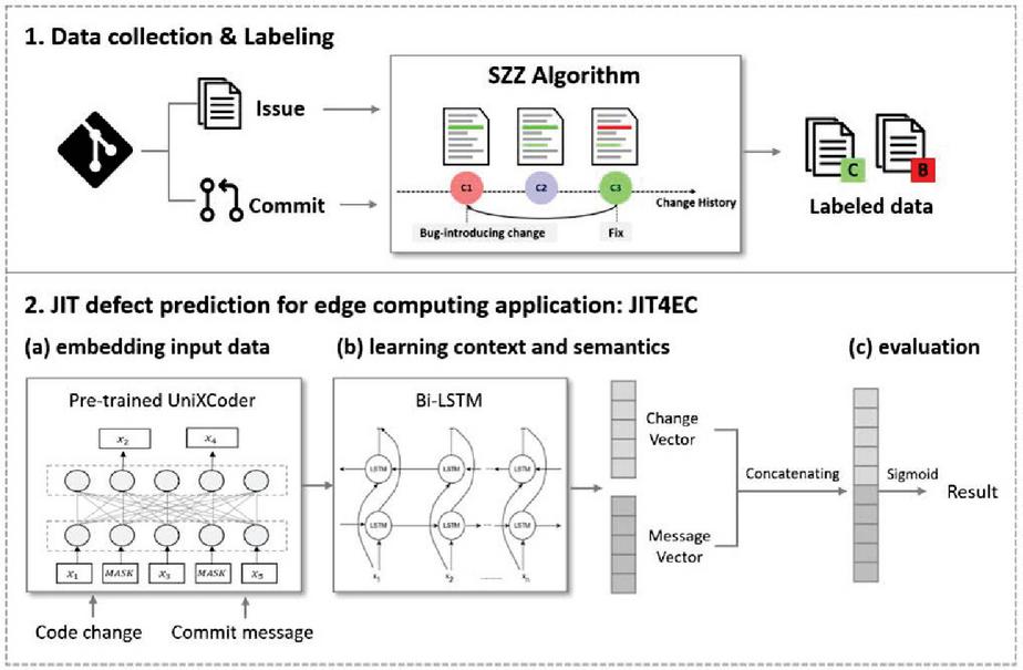
Figure 1 Data collection and labeling.
Unlike the above studies, we utilize the hierarchical and semantic information of source code (characteristic of programming language) in terms of input data, and we propose a novel JIT defect prediction suitable for self-driving software.
3 Proposed Approach
Our approach consists of two main phases, including data collection, and building JIT4EA. The procedure of our approach is illustrated in Figure 1.
3.1 Data Collection and Labeling
We collect commit data from open-source self-driving software on GitHub and use PYDRILLER [16] to collect commit messages and code changes for the project. Then, labeling is performed using the MA-SZZ algorithm [11, 17]. The SZZ algorithm automatically identifies code changes that cause defects, and various SZZ algorithms have been proposed so far [18]. The MA-SZZ algorithm has added meta-changes to the existing algorithm (Annotation Graph, AG-SZZ [19]) that include branch changes or file attribute changes. Therefore, the data labeled by MA-SZZ showed a low false positive rate [17] and better recall and precision performance than other algorithms [11].
Algorithm 1 Pseudo-code of JIT4EA
1:
2: Commit message M
3: Code change C
4: report Recall, PF, Balance, PCI@20%LOC, Effort@20%Recall,
5: (1) embedding input data
6:
7:
8: (2) learning context and semantics
9:
10:
11: (3) evaluation
12:
13:
14:
15: End
The SZZ algorithm is performed in two phases: (1) SZZ searches for bug-fixing changes. To this end, SZZ searches for some keywords, such as bug, fix or fail in each commit message to verify whether a commit is a defect-fixing change or not. (2) SZZ aims to identify the bug-prone commit. Firstly, SZZ uses the git diff command of a version management system to check the changed code line between the modified commit version and the previous version. This identified code line is classified as causing a defect, and the git blame command is used to find the last commit to modify and delete the code line from the previous fix. Finally, these changes are labeled as defects, and the other changes are labeled as non-defects.
3.2 Just-in-time Defect Prediction for Edge Computing Application
We build a new JIT defect prediction model based on labeled data performed in Section 3.1. Our proposed JIT defect prediction with deep learning for an edge computing application (JIT4EA) framework mitigates the limitations of related work described in Section 2. JIT4EA consists of three steps: (1) embedding input data, (2) learning context and semantics, and (3) evaluation. Algorithm 1 presents the pseudo-code of JIT4EA.
The quality of the embedded data affects the performance, so it is very important to use the appropriate embedding techniques for the data. We use commit messages and code changes as input data. Leverage pre-trained UniXCoder is used to embed them. UniXCoder reflects changes in the meaning of words according to context and performs embeddings that take into account the hierarchical structure and semantic information of the source code, and the relationship between commit messages and codes.
We first perform preprocessing of commit messages and code changes for input data embeddings (lines 1–3). At this step, we execute tokenization using UniXCoder, excluding punctuation characters. After this step, we obtain input data tokens of the maximum token length of each data. It then uses UniXCoder to embed commit messages and code changes. The commit message m is input in [] in UniXCoder to obtain sentence embedding as follows:
| (1) |
where r denotes an embedding dimension, CLS denotes the beginning of a sentence, and SEP denotes the end of a sentence. Code change C potentially contains the changed code lines of several source code files [], where represents the changed code lines of the ith modified source code file. To reflect the characteristic of these code changes [9], the changed code lines in one source code file () are connected to one sentence () and used as input data for UniXCoder.
| (2) |
The second step is to learn context and semantic representations from embedding representations obtained in previous steps (lines 4–6). This step is important because if the length of the data is long and the layers of the deep learning model are deep, the information of the input data can be lost. Therefore, we utilize Bi-LSTM models that are effective for context and semantic information learning to prevent these problems. The Bi-LSTM model is characterized in that it is possible to learn a relationship with the previous and the subsequent data on the input data. These characteristics help to effectively send information about embedded commit messages and code changes to the classifier.
To evaluate our proposed model, we use a fully connected layer (FC) to identify whether the commit is defect-prone (lines 7–10). The commit messages and code changes derived from the previous steps are combined into one to create new learning data that can represent changes. FC is learned with this train data, and the loss function uses the sigmoid function.
4 Experimental Setup
In this section we discuss our research questions. We then present the details of the datasets and the evaluation indicators used in experiments. We describe the baseline of four traditional classifiers and four state-of-the-art JIT defect prediction approaches. Finally, the detailed experimental design is explained.
4.1 Research Questions
To verify the effectiveness our proposed JIT4EA, we conduct experiments with the following two research questions (RQs):
RQ1. Can the proposed method perform better than other JIT defect prediction models?
RQ2. What factors affect the performance of the proposed method?
RQ1 is designed to show that our proposed method is superior to baselines. So, we compare the performance of JIT4EA with those of related work and traditional classifiers. Through RQ1, we also verify that JIT4EA is also effective in terms of cost. Code inspection effort is directly related to cost and is a metric of whether limited resources can be used effectively. RQ2 focuses on investigating which factors contribute to performance improvement. To this end, we perform sensitivity analysis on performance differences according to whether context and semantic learning is applied or not, and the type of input data.
4.2 Dataset
We collect open-source self-driving software data on GitHub. We use self-driving and autonomous driving as the keyword to search repositories on GitHub. Then, we sort them in descending order by most stars. In GitHub, the number of stars indicates the popularity of the repository, and the higher the number of stars, the more popular the repository. To choose the most suitable projects, we set up the following criteria:
(1) Excludes tutorials and educational projects.
(2) Excludes repositories that do not display the project language.
After filtering by these criteria, we choose the top three most starred popular project. Table 1 summarizes these projects, including programming language (% Language ratio), Stars, the number of times the source code file has been modified (# Change), the number of defects (# Defect), and the ratio of defects (% DR). Apollo is a project with the ability to accelerate the development, testing, and distribution of self-driving. Carla is a project that simulates self-driving. Although it is not self-driving software itself, it is included in that it is widely used for simulation. Donkeycar is a minimalist and modular self-driving library for Python.
Table 1 Summary of the project used in this work
| Project | % Language Ratio | Stars | # Change | # Defect | % DR |
| Apollo | C++(83.8), Python(5) Starlark(4.4), Shell(3.3) | 20.9K | 8,113 | 2,836 | 34.96 |
| Carla | C++(67.9), Python(25.6) Batchfile(2.6), Shell(2.1) | 7.2K | 6,477 | 2,933 | 45.28 |
| Donkeycar | Python(85.5), JavaScript(10.3), HTML(2.9), kvlang(2.1) | 2.2K | 2,359 | 865 | 36.67 |
4.3 Evaluation Indicators
We evaluate the performance of the proposed method using three effort-aware metrics that consider code inspection efforts and three effort-unaware metrics.
4.3.1 Effort-aware performance measures
PCI@20%LOC is an indicator of the percentage of actual defect-prone commits that can be found given a fixed amount of effort, i.e., top 20% LOC of the project [8]. A higher value of PCI@20%LOC means that an approach can rank many actual defect-prone commits so developers will expend less effort in finding actual defect-prone commits. When there are M changes and the developer inspected m changes, this is computed as
| (3) |
Effort@20%Recall is the effort (LOC) required to identify 20% of the defect-prone commit in the project. The higher the value of this indicator, the more effort the developer needs to identify the actual defect-prone commit. When there are N defect-prone changes and the developer finds n defect-prone changes, it is calculated as shown in Equation (4).
| (4) |
defines the relationship between recall and code inspection efforts for prediction models. This requires optimal and worst models, each sorted in descending and ascending order according to the actual defect density. A good prediction model is expected to approach the optimal model and calculated according to the following formula (5) for the proposed prediction model m.
| (5) |
4.3.2 Effort-unaware performance measures
| Predicted Class | |||
| Clean | Defect | ||
| Actual class | Clean | TP (true positive) | FN (false negative) |
| Defect | FP (false positive) | TN (true negative) | |
Recall refers to the proportion of defects correctly classified among actual defects. Equation (6) is calculated based on the confusion matrix of Table 2.
| (6) |
The probability of false alarm (PF) refers to the percentage of commits incorrectly classified as defective and is measured according to (7). The formula is calculated based on the confusion matrix. In addition, the lower the performance of PF, the better the performance.
| (7) |
Balance is an indicator that Recall and PF are considered comprehensively, which is widely used in defect prediction [18, 20] and is particularly suitable for class imbalance datasets. This indicator is measured according to (8).
| (8) |
4.3.3 Statistical analysis
In this work, we use Cohen’s d [21] to show that the difference in performance between the proposed method and the baseline is statistically significant. Cohen’s d is an effect-size test that numerically expresses the performance difference between the two techniques. Cohen’s d is classified into four levels as shown in Table 3, and each level represents the degree of the performance difference. For example, the ‘small’ level means that the performance difference between the two techniques is statistically small. The effect size above the ‘medium’ level means that the proposed technique has superior performance compared to other techniques.
| (9) |
Table 3 Effectiveness level based on Cohen’s d
| Cohen’s d | Level |
| Negligible (N) | |
| Small (S) | |
| Medium (M) | |
| Large (L) |
4.4 Baseline
To validate the performance of the proposed technique, we compare the performance of four traditional machine learning classifiers and four state-of-the-art JIT defect prediction approaches [6–9].
We select four traditional classifiers that are widely used in related work [19, 22]. They use the features of commit-level as input data and conduct experiments by applying preprocessing steps (min-max normalization, class imbalance problem solving using synthetic minority oversampling technique), which are commonly used in defect prediction studies [23].
4.4.1 Traditional classifiers
• Random forest (RF) is a classifier that generates multiple decision trees for subsets and averages them to improve accuracy and returns the final prediction.
• The gradient boosting decision tree (GBDT) works according to the principle of combining several weak (basic) classifiers to create one strong classifier, namely the ensemble technique. Each base classifier is a decision tree, and all decision trees are sequentially linked to learn the mistakes in previous decision tree models. As a result, the final model becomes a classifier that aggregates the results of each model to reduce errors.
• Logistic regression (LR) is a model that finds the relationship between variable response and predictor variable. The model fits the data to the logistic curve, and the parameters of the model are estimated based on maximum likelihood.
• Extreme gradient boosting (XGBoost), like GBDT, operates according to ensemble techniques, and the final model is generated by combining all previous models with a comprehensive model with high accuracy. It is characterized by providing fast learning of parallel processing with high accuracy.
4.4.2 State-of-the-art JIT approaches
• DeepJIT [6] performs word-based embeddings from commit messages and code corrections data with end-to-end learning techniques and then automatically extracts features using CNN models. After that, the defect prediction performance was confirmed through the fully connected layer.
• CC2Vec [7] used HAN networks to learn information between added and deleted codes from code modification data and further learn the hierarchical structure of commits. Code change vectors extracted through the network were combined with feature data extracted from a DeepJIT [9] model to perform defect prediction.
• JITLine [8] uses the number of code frequencies in the feature and code change data in the commit-level as train data, and applies an oversampling technique, SMOTE, to address the class imbalance problem in the defect data. In addition, the parameters of SMOTE were optimized with a differential evolution algorithm. Thereafter, defect prediction was performed using a random forest model.
• CodeBERT4JIT [9] found that the DeepJIT [6] CNN model was used as an encoder, and presented an approach to replace it with CodeBERT. They use CodeBERT to embed commit messages and code change and perform defect prediction through a fully connected layer.
4.5 Experimental Setting
We use a stratified k-fold cross-validation method to measure the generalized performance of the proposed technique and related work. This is a method that is widely used in defect prediction work [6, 23], and in this study, an experiment is conducted by setting k to 10. In addition, the experimental environments conducted in this work used Python 3.6 and 3.8 in Windows 10. Python 3.6 was used to implement the comparison techniques (machine learning classifier, DeepJIT [6], CC2Vec [7], and JITLine [8]), and Python 3.8 was used to implement the proposed method, and CodeBERT4JIT [9].
We use the 14 commit-level features in RQ2. These features are divided into five dimensions: diffusion, size, purpose, history, and experience [13]. The diffusion feature quantifies the distribution within the change, and the size feature measures the size of the change such as lines of code added. The purpose feature characterizes whether to fix bugs, and the history feature indicates how developers modify the files within the change. The experience feature quantifies the change experience of developers who perform change based on the number of changes previously submitted by the developer.
5 Experimental Results
5.1 RQ1. Can the Proposed Method Perform Better than Other JIT Defect Prediction Models?
In this research question, we compare the performance of machine learning models and state-of-the-art approaches to validate the performance of the JIT4EA. Table 4 reports the performance of the indicators that do not consider the code inspection efforts. The bold text in the table means the best performance in the indicator, and the ‘Bal’ column means the Balance performance indicator.
Table 4 Results of evaluation indicators without considering code inspection effort
| Donkeycar | Carla | Apollo | |||||||
| Evaluation | Recall | PF | Bal | Recall | PF | Bal | Recall | PF | Bal |
| RF | 0.703 | 0.301 | 0.681 | 0.599 | 0.444 | 0.550 | 0.245 | 0.205 | 0.422 |
| GBDT | 0.714 | 0.316 | 0.687 | 0.522 | 0.387 | 0.545 | 0.287 | 0.316 | 0.421 |
| XGBoost | 0.697 | 0.297 | 0.686 | 0.489 | 0.359 | 0.549 | 0.268 | 0.295 | 0.412 |
| LR | 0.800 | 0.390 | 0.680 | 0.765 | 0.510 | 0.572 | 0.806 | 0.539 | 0.572 |
| DeelJIT | 0.685 | 0.331 | 0.677 | 0.727 | 0.402 | 0.652 | 0.724 | 0.405 | 0.652 |
| CC2Vec | 0.737 | 0.685 | 0.525 | 0.767 | 0.716 | 0.467 | 0.768 | 0.677 | 0.421 |
| JITLine | 0.752 | 0.251 | 0.750 | 0.793 | 0.301 | 0.745 | 0.542 | 0.127 | 0.707 |
| CodeBERT4JIT | 0.813 | 0.212 | 0.772 | 0.861 | 0.140 | 0.852 | 0.889 | 0.111 | 0.885 |
| JIT4EA | 0.912 | 0.092 | 0.909 | 0.938 | 0.060 | 0.938 | 0.912 | 0.106 | 0.895 |
From Table 4, the proposed method for all three projects shows superior performance in all performance indicators. We find that JIT4EA achieves the highest Recall value, which means that the proposed method well identifies defects compared to the baseline. In particular, we can observe that JIT4EA and CodeBERT4JIT outperform other baselines. From these results, we can confirm two things: (1) the contextual semantic information is important; (2) the relationship between commit messages and code changes is important (this is the difference between other baselines [6–8] and two approaches (CodeBERT4JIT [9] and JIT4EA)). Our proposed JIT4EA has better performance than CodeBERT4JIT. The main difference between UniXCoder and CodeBERT is the hierarchical structure of the code and whether semantic information is learned. Our experimental results confirm that the hierarchical structure and semantic information of the code are important for JIT defect prediction.
Table 5 Results of evaluation indicators with considering code inspection effort
| Donkeycar | Carla | Apollo | |||||||
| Evaluation | PCI | Effort | PCI | Effort | PCI | Effort | |||
| RF | 0.355 | 0.107 | 0.792 | 0.236 | 0.180 | 0.611 | 0.198 | 0.248 | 0.439 |
| GBDT | 0.358 | 0.107 | 0.795 | 0.253 | 0.162 | 0.624 | 0.198 | 0.219 | 0.518 |
| XGBoost | 0.348 | 0.108 | 0.791 | 0.239 | 0.176 | 0.584 | 0.184 | 0.235 | 0.499 |
| LR | 0.338 | 0.124 | 0.777 | 0.277 | 0.142 | 0.707 | 0.324 | 0.118 | 0.710 |
| DeelJIT | 0.313 | 0.119 | 0.751 | 0.297 | 0.128 | 0.731 | 0.374 | 0.090 | 0.733 |
| CC2Vec | 0.234 | 0.167 | 0.556 | 0.226 | 0.176 | 0.555 | 0.284 | 0.136 | 0.624 |
| JITLine | 0.388 | 0.097 | 0.834 | 0.334 | 0.116 | 0.826 | 0.422 | 0.089 | 0.802 |
| CodeBERT4JIT | 0.344 | 0.114 | 0.870 | 0.24 | 0.114 | 0.922 | 0.546 | 0.068 | 0.951 |
| JIT4EA | 0.367 | 0.106 | 0.974 | 0.345 | 0.113 | 0.982 | 0.553 | 0.068 | 0.964 |
Table 5 reports the experimental results of the performance indicator considering the code inspection effort, and the bold text in the table means that the performance is the best. The column ‘PCI’ means PCI@20%LOC evaluation indicator, and the column ‘Effort’ indicates Effort@20%Recall. The proposed method obtains superior performance, which means that the proposed method can reduce the code inspection effort. The result of the PCI@20%LOC performance indicates that the proposed method can identify many actual defect-prone commits given limited effort compared to the baselines. In addition, Effort@20%Recall performance is better than the baselines in the two projects except for the Donkeycar project, which means that the developers need less effort to identify actual defects. In the Donkeycar project, the proposed method ranks number two; less effort is required for developers to identify actual defects. shows that the proposed method is an effective model that can identify many defect-introducing commits with less code inspection effort.
Table 6 Effect size analysis results
| JIT4EA vs. | ||||||
| Recall | PF | Balance | PCI | Effort | ||
| RF | 2.91 (L) | 3.26 (L) | 4.78 (L) | 1.95 (L) | 1.93 (L) | 3.51 (L) |
| GBDT | 3.33 (L) | 9.31 (L) | 4.67 (L) | 1.88 (L) | 1.9 (L) | 4.05 (L) |
| XGBoost | 3.5 (L) | 9.28 (L) | 4.55 (L) | 2.01 (L) | 1.98 (L) | 4.00 (L) |
| LR | 8.4 (L) | 8.27 (L) | 8.04 (L) | 1.59 (L) | 2.09 (L) | 10.39 (L) |
| DeepJIT | 13.05 (L) | 10.53 (L) | 16.99 (L) | 1.34 (L) | 0.93 (L) | 28.88 (L) |
| CC2Vec | 12.28 (L) | 33.62 (L) | 13.58 (L) | 2.55 (L) | 3.49 (L) | 16.9 (L) |
| JITLine | 2.88 (L) | 2.61 (L) | 9.07 (L) | 0.57 (M) | 0.31 (S) | 13.99 (L) |
| CodeBERT4JIT | 2.8 (L) | 2.05 (L) | 2.15 (L) | 0.4 (S) | 0.16 (N) | 2.45 (L) |
Effect size analysis using Cohen’s d is conducted to verify whether the difference in performance between our proposed method and the baseline was statistically significant. From Table 6, we can observe that there is a significant performance difference between JIT4EA and baselines in indicators that do not consider the code inspection effort. In terms of effort-aware indicators, JIT4EA can produce a large effect size compared to the performance of traditional classifiers, DeepJIT, and CC2Vec. In Effort@20%Recall, the performance difference between JITLine and the proposed method is small, which means that the performance difference between the two methods is small. It also implies that there is little difference in Effort@20%Recall performance between CodeBERT4JIT and the proposed method.
The proposed method obtains improvement in performance indicators that do not consider code inspection efforts, and most of the performance indicators considering code inspection efforts showed performance differences of a small level or higher.
5.2 RQ2. What Factors Affect the Performance of the Proposed Method?
We conduct a sensitivity analysis from two perspectives to identify factors affecting the performance of the JIT4EA model in this research question. First, we check the performance difference according to the input data. We use commit messages and code change data together. So we compare the performance in four cases: (1) when using only commit messages, (2) when using only code changes, (3) when both data are put together, and (4) when using existing commit-level feature data with commit message and code change data.
Table 7 Performance differences based on factors affecting the performance of JIT4EA
| Project | Sensitivity | Recall | PF | Bal | PCI | Effort | |
| Donkeycar | JIT4EA | 0.9124 | 0.0929 | 0.9097 | 0.3679 | 0.106 | 0.9744 |
| w/o code | 0.9118 | 0.0994 | 0.902 | 0.3593 | 0.1091 | 0.9582 | |
| w/o meg | 0.9146 | 0.099 | 0.9046 | 0.3671 | 0.1066 | 0.9696 | |
| Add Feature | 0.9238 | 0.0946 | 0.9105 | 0.3666 | 0.1065 | 0.9732 | |
| w/o Bi-LSTM | 0.9094 | 0.1001 | 0.9046 | 0.3665 | 0.1066 | 0.9689 | |
| Carla | JIT4EA | 0.9385 | 0.0603 | 0.9381 | 0.3457 | 0.1131 | 0.9823 |
| w/o code | 0.8942 | 0.0678 | 0.9104 | 0.3401 | 0.1148 | 0.9568 | |
| w/o meg | 0.9119 | 0.0847 | 0.9135 | 0.3449 | 0.1132 | 0.9702 | |
| Add Feature | 0.926 | 0.054 | 0.9327 | 0.3446 | 0.1136 | 0.9803 | |
| w/o Bi-LSTM | 0.9006 | 0.1115 | 0.8903 | 0.342 | 0.1141 | 0.9549 | |
| Apollo | JIT4EA | 0.9602 | 0.0462 | 0.9557 | 0.5728 | 0.0673 | 0.9905 |
| w/o code | 0.9433 | 0.1278 | 0.8903 | 0.5544 | 0.0691 | 0.9612 | |
| w/o meg | 0.903 | 0.1068 | 0.8971 | 0.5538 | 0.0686 | 0.9651 | |
| Add Feature | 0.968 | 0.0754 | 0.9413 | 0.562 | 0.0693 | 0.9824 | |
| w/o Bi-LSTM | 0.9125 | 0.1062 | 0.8956 | 0.5531 | 0.0686 | 0.9647 |
Table 7 shows the experimental results for this, where the ‘w/o code’ line in the table used only commit messages, the ‘w/o meg’ line used only code changes, and ‘JIT4EA’ used a combination of commit messages and code changes. In addition, the ‘Bal’ column means a Balance performance indicator, ‘PCI’ indicates a PCI@20%LOC, and ‘Effort’ means an Effort@20%Recall. As can be seen in Table 7, when the characteristic of the commit-level was used together, superior performance was shown in the evaluation indicator considering the code inspection effort. However, the evaluation inspection considering the code inspection effort showed excellent performance when the commit message and code change data were used together. This means that when commit messages and code change data are used, more defects can be identified in limited testing resources and less effort is required to identify actual defects.
Table 8 Analyze the effect size of the factors affecting performance
| JIT4EA vs. | ||||
| Input Data | Sensitivity Factor | |||
| w/o code | w/o meg | Add feature | w/o Bi-LSTM | |
| Recall | 1.03 (L) | 1.9 (L) | 0.11 (N) | 2.17 (L) |
| PF | 1.43 (L) | 1.98 (L) | 0.45 (S) | 2.77 (L) |
| Balance | 2.29 (L) | 2.07 (L) | 0.38 (S) | 2.68 (L) |
| PCI | 0.1 (N) | 0.07 (N) | 0.04 (N) | 0.036 (N) |
| Effort | 0.1 (N) | 0.03 (N) | 0.05 (N) | 0.04 (N) |
| 4.9 (L) | 2.86 (L) | 0.69 (M) | 3.14 (L) |
In Table 8, the ‘input’ column is a result of performing an effect size test according to input data. JIT4EA shows significant performance improvements over only commit messages and when only code changes in indicators without considering code inspection efforts. In addition, when comparing the performance of JIT4EA (with commit messages and code changes) and commit-level feature data together, we can be confirmed that the performance difference is statistically small or negligible. Among the indicators considering the code inspection effort, the shows that there is a performance difference of more than medium-level when both of them are used together compared to when only commit messages and only code change are used. On the other hand, it can be seen that there is little difference in performance according to input data in indicators excluding .
Second, the effort of context and semantic learning steps on performance was confirmed. To this end, we compared the case with and without Bi-LSTM, and Table 7 shows the experimental results for this. As a result, it was shown that there was a slight improvement in performance in all projects when Bi-LSTM was used. In particular, we show that the Balance is improved in Carla and Apollo projects, and the performance indicators considering the code inspection effort show that the performance is slightly improved through context and semantic information learning through all projects.
In Table 7, the ‘Sensitivity factor’ column is the result of analyzing the effect size according to the context and semantic learning stage, and indicators that do not consider the code inspection effort show that there is a performance difference as large-level in all evaluation indicators. This means that the context and semantic learning steps contribute to performing defect prediction well. In the performance indicator considering the code inspection effort, it was confirmed that the context and semantic learning stage did not affect the code inspection effort excluding . The has shown that context and semantic learning steps can reduce code inspection efforts. Therefore, it can be confirmed that the context and semantic learning steps are important in the proposed JIT4EA.
6 Threat to Validity
6.1 External Validity
We choose the top three most star projects (Donkeycar, Carla, and Apollo) on Github. The project has attracted the attention of many developers in the version management system GitHub, and in the case of the Apollo project, it is the industry’s open-source self-driving software. We plan to collect more self-driving software projects to verify the performance of the proposed method.
6.2 Internal Validity
In this work, performance comparisons are performed with state-of-the-art JIT defect prediction to verify the performance of the proposed method. In this process, there is a threat that the performance written in the paper of the related work may not have been equally reflected in the process of conducting this study. To mitigate this threat, the related research implementation was conducted by referring to the code shared with the paper of the related research, and the process of verifying the related research implementation code was performed.
7 Conclusion
JIT defect prediction helps developers reduce code inspection and testing efforts, helping to improve the quality of the software under development. Many researchers have proposed various JIT defect prediction approaches, but there are no JIT defect prediction models for self-driving software with edge computing applications. So we proposed a JIT defect prediction model for self-driving software.
In this study, self-driving software data were collected and labeled to perform JIT defect prediction of self-driving software. We then applied our proposed method, and our method performs defect prediction by embedding hierarchical structure and semantic information. This is different from the existing JIT defect prediction method, and it is experimentally confirmed that the hierarchical structure and semantic information of the code contribute to the improvement of defect prediction performance. The proposed method outperforms traditional machine learning models and state-of-the-art approaches, and in particular, it has been able to reduce code inspection efforts.
We analyzed the difference in performance according to the components of the proposed method and the input data used to identify factors affecting the defect prediction performance of the proposed technique in this study. As a result, the combination of commit messages and code changes reduced the code inspection effort, and the combination of commit-level features showed excellent performance in evaluation indicators without considering the code inspection effort. In addition, sensitivity analysis was performed to emphasize the importance of the context and semantic learning steps of the proposed method in this work, and as a result, the context and semantic learning steps slightly improved the performance of defect prediction. Therefore, the method proposed is expected to identify defects in self-driving software from the development stage and consequently contribute to improving software quality.
References
[1] Watch: “Tesla Model 3 on Autopilot hit by a semi-truck and pushed for half mile”, HT auto, Updated on 18 Oct 2021, https://auto.hindustantimes.com/auto/cars/watch-tesla-model-3-on-autopilot-hit-by-a-semi-truck-and-pushed-for-half-mile-41634546063019.html
[2] L. Jiang, S. Jiang, L. Gong, Y. Dong, Q. Yu, “Which process metrics are significantly important to change of defects in evolving projects: An empirical study,” IEEE Access, vol. 8, pp. 93705–93722, 2020.
[3] S. Wang, T. Liu, J. Nam, L. Tan, “Deep semantic feature learning for software defect prediction,” IEEE Transactions on Software Engineering, vol. 46, no. 12, pp. 1267–1293, 2018.
[4] L. Šikić, A. S. Kurdija, K. Vladimir, M. Šilić, Graph neural network for source code defect prediction,” IEEE Access, vol. 10, pp. 10402–10415, 2022.
[5] D. Guo, S. Lu, N. Duan, Y. Wang, M. Zhou, J. Yin, “UniXcoder: Unified cross-modal pre-training for code representation,” arXiv preprint arXiv:2203.03850, 2022.
[6] T. Hoang, H. K. Dam, Y. Kamei, D. Lo, N. Ubayashi, “DeepJIT: an end-to-end deep learning framework for just-in-time defect prediction,” in 2019 IEEE/ACM 16th International Conference on Mining Software Repositories (MSR), 2019, pp. 34–45.
[7] T. Hoang, H. J. Kang, D. Lo, J. Lawall, “Cc2vec: Distributed representations of code changes,” in Proceedings of the ACM/IEEE 42nd International Conference on Software Engineering, 2020, pp. 518–529.
[8] C. Pornprasit and C. K. Tantithamthavorn, “Jitline: A simpler, better, faster, finer-grained just-in-time defect prediction,” in 2021 IEEE/ACM 18th International Conference on Mining Software Repositories (MSR), 2021, pp. 369–379.
[9] X. Zhou, D. Han, D. Lo, “Assessing generalizability of CodeBERT,” in 2021 IEEE International Conference on Software Maintenance and Evolution (ICSME), 2021, pp. 425–436.
[10] C. Jiwon, S. Manikandan, R. Duksan, B. Jongmoon, “An empirical analysis on just-in-time defect prediction models for self-driving software systems,” 2nd International Workshop on Big Data-driven Edge Cloud Services (BECS), 2022.
[11] G. Rosa, L. Pascarella, S. Scalabrino, R. Tufano, G. Bavota, M. Lanza, R. Oliveto, “Evaluating SZZ implementations through a developer-informed oracle,” in 2021 IEEE/ACM 43rd International Conference on Software Engineering (ICSE), 2021, pp. 436–447.
[12] L. Šikić, A. S. Kurdija, K. Vladimir, M. Šilić, “Graph neural network for source code defect prediction,” IEEE Access, vol. 10, pp. 10402–10415, 2022.
[13] Y. Kamei, E. Shihab, B. Adams, A. E. Hassan, A. Mockus, A. Sinha, N. Ubayashi, “A large-scale empirical study of just-in-time quality assurance,” IEEE Transactions on Software Engineering, vol. 39, no. 6, pp. 757–773, 2012.
[14] Z. Yang, D. Yang, C. Dyer, X. He, A. Smola, E. Hovy, “Hierarchical attention networks for document classification,” in Proceedings of the 2016 Conference of the North American Chapter of the Association for Computational Linguistics: Human Language Technologies, pp. 1480–1489, 2016.
[15] Z. Feng, D. Guo, D. Tang, N. Duan, X. Feng, M. Gong, et al., “Codebert: A pre-trained model for programming and natural languages,” arXiv preprint arXiv:2002.08155, 2020.
[16] D. Spadini, M. Aniche, A. Bacchelli, “Pydriller: Python framework for mining software repositories,” in Proceedings of the 2018 26th ACM Joint Meeting on European Software Engineering Conference and Symposium on the Foundations of Software Engineering, 2018, pp. 908–911.
[17] Y. Fan, X. Xia, D. A. Da Costa, D. Lo, A. E. Hassan, S. Li, “The impact of mislabeled changes by SZZ on just-in-time defect prediction,” IEEE Transactions on Software Engineering, vol. 47, no. 8, pp. 1559–1586, 2019.
[18] D. Ryu and J. Baik, “Effective multi-objective naïve Bayes learning for cross-project defect prediction,” Applied Soft Computing, vol. 49, pp. 1062–1077, 2016.
[19] G. Esteves, E. Figueiredo, A. Veloso, M. Viggiato, N. Ziviani, “Understanding machine learning software defect predictions,” Automated Software Engineering, vol. 27, no. 3, pp. 369–392, 2020.
[20] K. E. Bennin, J. W. Keung, A. Monden, “On the relative value of data resampling approaches for software defect prediction,” Empirical Software Engineering, vol. 24, no. 2, pp. 602–636, 2019.
[21] G. Esteves, E. Figueiredo, A. Veloso, M. Viggiato, N. Ziviani, “Understanding machine learning software defect predictions,” Automated Software Engineering, vol. 27, no. 3, pp. 369–392, 2020.
[22] Y. Kamei, E. Shihab, B. Adams, A. E. Hassan, A. Mockus, A. Sinha, N. Ubayashi, “A large-scale empirical study of just-in-time quality assurance,” IEEE Transactions on Software Engineering, vol. 39, no. 6, pp. 757–773, 2012.
[23] J. Lee, J. Choi, D. Ryu, S. Kim, “Holistic parameter optimization for software defect prediction,” IEEE Access, vol. 10, pp. 106781–106797, 2022.
Biographies

Jiwon Choi received her B.S. degree and M.S. degree in Software Engineering from Jeonbuk National University in 2020 and 2022 respectively. Currently, she is a contract research scientist in the school of computing at Korea Advanced Institute of Science and Technology (KAIST). Her research areas include software defect prediction, deep learning, edge computing QoS prediction, and software reliability engineering.

Taeyoung Kim is a Ph.D. student of the Department of Software Engineering at Jeonbuk National University. His research areas include Blockchain, software engineering and artificial intelligence.

Duksan Ryu earned a bachelor’s degree in computer science from Hanyang University in 1999 and a Master’s dual degree in software engineering from KAIST and Carnegie Mellon University in 2012. He received his Ph.D. degree from the school of computing, KAIST in 2016. His research areas include software analytics based on AI, software defect prediction, mining software repositories, and software reliability engineering. He is currently an associate professor in the software engineering department at Jeonbuk National University.

Jongmoon Baik received his B.S. degree in computer science and statistics from Chosun University in 1993. He received his M.S. degree and Ph.D. degree in computer science from University of Southern California in 1996 and 2000 respectively. He worked as a principal research scientist at Software and Systems Engineering Research Laboratory, Motorola Labs, where he was responsible for leading many software quality improvement initiatives. His research activity and interest are focused on software six sigma, software reliability and safety, and software process improvement. Currently, he is an associate professor in the school of computing at Korea Advanced Institute of Science and Technology (KAIST). He is a member of the IEEE.

Suntae Kim is a professor of the Department of Software Engineering at Chonbuk National University. He received his Ph.D. degree in Computer Science & Engineering from Sogang University in 2010. His research areas include Blockchain, software engineering and artificial intelligence.
Journal of Web Engineering, Vol. 22_2, 303–326.
doi: 10.13052/jwe1540-9589.2225
© 2023 River Publishers
